An Accelerated Dual-Integral Structure Zeroing Neural Network Resistant to Linear Noise for Dynamic Complex Matrix Inversion

Abstract

The problem of inverting dynamic complex matrices remains a central and intricate challenge that has garnered significant attention in scientific and mathematical research. The zeroing neural network (ZNN) has been a notable approach, utilizing time derivatives for real-time solutions in noiseless settings. However, real-world disturbances pose a significant challenge to a ZNN’s convergence. We design an accelerated dual-integral structure zeroing neural network (ADISZNN), which can enhance convergence and restrict linear noise, particularly in complex domains. Based on the Lyapunov principle, theoretical analysis proves the convergence and robustness of ADISZNN. We have selectively integrated the SBPAF activation function, and through theoretical dissection and comparative experimental validation we have affirmed the efficacy and accuracy of our activation function selection strategy. After conducting numerous experiments, we discovered oscillations and improved the model accordingly, resulting in the ADISZNN-Stable model. This advanced model surpasses current models in both linear noisy and noise-free environments, delivering a more rapid and stable convergence, marking a significant leap forward in the field.

1. Introduction

Matrix inversion is a fundamental and crucial problem encountered in various domains [1,2,3,4,5], including mathematics and engineering, chaotic systems [1,2,3], and robotic dynamics [5]. Numerous methods exist for solving this problem, primarily categorized into two approaches. The first is numerical computation methods, such as Newton’s iterative method [6,7], which, though fundamentally serial in nature, suffer from slow computation speed and high resource consumption, rendering them ineffective for efficiently computing the inverse of high-dimensional matrices. Another approach is neural-network-based methods, inherently parallel in computation, such as gradient neural networks (GNNs) [8,9,10,11], renowned for their high computational accuracy and exponential convergence. However, GNNs have their own set of challenges and limitations, particularly when it comes to handling dynamic or time-varying data.

Introduced 20 years ago, the ZNN model proposed by Zhang et al. [12] is a specialized neural network architecture that is more adaptive and efficient for solving real-time matrix inversion problems. However, ZNNs are only applicable in ideal noise-free environments. In reality, various types of noise exist, impairing ZNNs’ convergence to theoretical values. Dynamic matrix inversion encompasses two domains: dynamic real matrix inversion and dynamic complex matrix inversion. According to PID control theory [13], the Integration-Enhanced Zhang Neural Network model (IEZNN) [14], proposed by Jin et al., restricts noise interference and is employed to address dynamic real matrix inversion problems, demonstrating commendable noise restriction capabilities and convergence performance through theoretical analysis and experimental validation.

The applications of dynamic matrix inversion in the complex domain span various scientific and engineering disciplines [15,16,17,18,19]. Mathematical models in the complex domain are crucial for describing phenomena such as control systems [16], signal processing [17], and optical systems [18]. Therefore, this paper focuses on the problem of dynamic complex matrix inversion.

Expanding upon previous research on zeroing neural network (ZNN) models, Zhang et al. proposed a complex-valued ZNN (CVZNN) to address DCMI problems [20]. Xiao et al. introduced a complex-valued noise-tolerant ZNN (CVNTZNN) model [21] aimed at restricting real-world noise interference, inspired by the noise reduction principle of integral-based zeroing neural networks. However, the CVNTZNN model struggles to effectively restrict linear noise. Recently, Hua et al. introduced the dual-integral structure zeroing neural network (DISZNN) model [22]. Leveraging its inherent dual-integral structure, the DISZNN model demonstrates superior performance in restricting linear noise for DCMI problems, as evidenced by theoretical analysis based on Laplace transforms. Moreover, numerous studies suggest that integrating activation functions (AFs) into ZNN models enhances noise tolerance and convergence performance [23,24,25,26,27,28,29,30,31]. Therefore, this paper proposes an accelerated dual-integral structure zeroing neural network (ADISZNN) by combining AFs with the DISZNN model to enhance its noise restriction capabilities against linear noise and accelerate convergence. It is noteworthy that the DISZNN model is restructured in this study, and the convergence and robustness of the ADISZNN model are theoretically analyzed and demonstrated in a different manner.

This article delineates the following scholarly contributions: The integration of DISZNN with a novel activation function has culminated in the development of an accelerated dual-integral structure zeroing neural network (ADISZNN). This model utilizes a dual-integral structure and activation function, demonstrating improved convergence speed. This means that the model’s computed results can more quickly approach the theoretical inverse of the target matrix. Oscillatory fluctuations observed in the steady-state residual error of ADISZNN, particularly with the SBPAF activation function, have been identified and mitigated through targeted enhancements. Theoretical analyses, supported by results from three comparative numerical experiments, confirm the outstanding convergence and robustness of the enhanced stable ADISZNN model. To our knowledge, no prior work has introduced an accelerated dual-integral structure zeroing neural network capable of linear noise cancellation in the context of dynamic complex matrix inversion.

The article is structured into five methodical sections. Section 2 delves into the DCMI problem, presenting the design formulation and procedural details of the ADISZNN model. Section 3 offers a theoretical exposition and validation of ADISZNN’s convergence and robustness, utilizing Lyapunov’s theorem and supported by graphical analyses, with the SBPAF function selected for the model’s activation. In Section 4, we conducted three sets of numerical comparison experiments. The article concludes with a summary of the findings in Section 5.

2. Problem Formulation, Design Formula, and ADISZNN Model

2.1. Consideration of the DCMI Problem

The dynamic complex matrix inverse problem can be described as follows:

$$\mathbf{A}\left(t\right)\mathbf{X}\left(t\right)=\mathbf{I},\mathrm{or}\mathbf{X}\left(t\right)\mathbf{A}\left(t\right)=\mathbf{I}\in {\mathbb{C}}^{n\times n},$$

(1)

where $\mathbf{A}\left(t\right)\in {\mathbb{C}}^{n\times n}$ is a nonsingular and smooth dynamic complex coefficient matrix with rank n, and $\mathbf{X}\left(t\right)$ represents the real-time solution of Equation (1), obtained through the ADISZNN model, where $\mathbf{I}\in {\mathbb{C}}^{n\times n}$ denotes the identity matrix. Our aim is to compute $\mathbf{X}\left(t\right)$ such that Equation (1) holds true at any given time $t\in [0,+\infty )$. Hence, we have ${\mathbf{X}}^{\ast }\left(t\right)={\mathbf{A}}^{-1}\left(t\right)$.

As complex numbers consist of real and imaginary parts, Equation (1) can be rewritten as

$$[{\mathbf{A}}_{\mathrm{re}}\left(t\right)+j{\mathbf{A}}_{\mathrm{im}}\left(t\right)][{\mathbf{X}}_{\mathrm{re}}\left(t\right)+j{\mathbf{X}}_{\mathrm{im}}\left(t\right)]=\mathbf{I},$$

(2)

where $[{\mathbf{A}}_{\mathrm{re}}\left(t\right)+j{\mathbf{A}}_{\mathrm{im}}\left(t\right)][{\mathbf{A}}_{\mathrm{re}}\left(t\right)+j{\mathbf{A}}_{\mathrm{im}}\left(t\right)]$ is the expansion of the complex matrix $\mathbf{A}\left(t\right)$, and ${\mathbf{A}}_{\mathrm{re}}\left(t\right)$ and ${\mathbf{A}}_{\mathrm{im}}\left(t\right)$ are, respectively, the real and imaginary parts of the given matrix $\mathbf{A}\left(t\right)$. Similarly, ${\mathbf{X}}_{\mathrm{re}}\left(t\right)$ and ${\mathbf{X}}_{\mathrm{im}}\left(t\right)$ are, respectively, the real and imaginary parts of the state solution $\mathbf{X}\left(t\right)$, where the imaginary unit is denoted as $j=\sqrt{-1}$.

2.2. Design Formula

To compute the dynamic complex matrix inversion, a function is devised to measure the real-time error in Equation (1), as follows:

$$\mathbf{E}\left(t\right)=\mathbf{A}\left(t\right)\mathbf{X}\left(t\right)-\mathbf{I}.$$

(3)

Its derivative with respect to time t is given by

$$\dot{\mathbf{E}}\left(t\right)=\dot{\mathbf{A}}\left(t\right)\mathbf{X}\left(t\right)+\mathbf{A}\left(t\right)\dot{\mathbf{X}}\left(t\right).$$

(4)

The design formula of the integration-enhanced zeroing neural network model is as follows [14]:

$$\dot{\mathbf{E}}\left(t\right)=-s_0\left(\mathbf{E}\left(t\right)\right)-s_1{\int }_0^t\mathbf{E}\left(\tau \right)d\tau$$

(5)

where design parameters $s_0>0$ and $s_1>0$ are adjusted for the rate. By combining Equations (4) and (5), we can derive the following formula:

$$\begin{array}{c}\hfill \mathbf{A}\left(t\right)\dot{\mathbf{X}}\left(t\right)=-\dot{\mathbf{A}}\left(t\right)\mathbf{X}\left(t\right)-s_0(\mathbf{A}\left(t\right)\mathbf{X}\left(t\right)-\mathbf{I})-s_1{\int }_0^t(\mathbf{A}\left(\tau \right)\mathbf{X}\left(\tau \right)-\mathbf{I})d\tau .\end{array}$$

(6)

In actuality, a wide array of noise phenomena are consistently present across numerous practical applications. Examples include the superfluous movements observed in robotic arm operations, as discussed in [32], and the chaotic dynamics within permanent magnet synchronous motor (PMSM) systems, as explored in [33], among others. To more accurately reflect real-world conditions, we introduce noise into Equation (6), thereby obtaining the following equation:

$$\begin{array}{c}\hfill \mathbf{A}\left(t\right)\dot{\mathbf{X}}\left(t\right)=-\dot{\mathbf{A}}\left(t\right)\mathbf{X}\left(t\right)-s_0(\mathbf{A}\left(t\right)\mathbf{X}\left(t\right)-\mathbf{I})-s_1{\int }_0^t(\mathbf{A}\left(\tau \right)\mathbf{X}\left(\tau \right)-\mathbf{I})d\tau +\mathbf{N}\left(t\right).\end{array}$$

(7)

2.3. Dual-Integral Structure ZNN Model Design

The DISZNN model proposed by Hua et al. [22] has demonstrated significant efficacy in the restriction of noise, particularly linear noise. The model for DISZNN is as follows:

$$\begin{array}{c}\hfill \dot{\mathbf{E}}\left(t\right)=-s_0^3{\int }_0^t{\int }_0^{\delta }\mathbf{E}\left(\tau \right)d\tau d\delta -3s_0^2{\int }_0^t\mathbf{E}\left(\delta \right)d\delta -3s_0\mathbf{E}\left(t\right)\end{array}$$

(8)

in which $s_0\in {\mathbb{R}}^{+}$ is the design parameter, the single-integral term restricts noise, while the double-integral term not only restricts noise but also accelerates convergence speed.

2.4. ADISZNN Model Design

It has been mentioned in many papers [23,24,25,26,27,28,29,30,31] that adding an activation function to some ZNN-like models can accelerate the convergence of the error function and enhance the model’s ability to restrict noise. Therefore, we modified the ZNN model by adjusting its design formula to

$$\dot{\mathbf{E}}\left(t\right)=-\alpha \Phi \left(\mathbf{E}\left(t\right)\right)$$

(9)

in which, $\Phi$(·): ${\mathbb{C}}^{n\times n}\to {\mathbb{C}}^{n\times n}$ is an activation function.

To provide a more intuitive description of the model’s evolution, we set

$$\Theta \left(t\right)=\dot{\mathbf{E}}\left(t\right)+\alpha \Phi \left(\mathbf{E}\left(t\right)\right)$$

(10)

Letting

$$\Theta \left(t\right)=-\lambda {\int }_0^t\Theta \left(\tau \right)d\tau ,$$

(11)

where $\lambda >0$.

We define

$$\mathbf{Y}\left(t\right)=\Theta \left(t\right)+\lambda {\int }_0^t\Theta \left(\tau \right)d\tau ,$$

(12)

and substituting Equation (10) into Equation (12), we can obtain

$$\begin{array}{cc}\hfill \mathbf{Y}\left(t\right)& =\dot{\mathbf{E}}\left(t\right)+\alpha \Phi \left(\mathbf{E}\left(t\right)\right)+\lambda {\int }_0^t(\dot{\mathbf{E}}\left(t\right)+\alpha \Phi \left(\mathbf{E}\left(\tau \right)\right))d\tau \hfill \\ \hfill & =\dot{\mathbf{E}}\left(t\right)+\alpha \Phi \left(\mathbf{E}\left(t\right)\right)+\lambda \mathbf{E}\left(t\right)+\lambda \alpha {\int }_0^t\Phi \left(\mathbf{E}\left(\tau \right)\right)d\tau .\hfill \end{array}$$

(13)

Similarly, we let

$$\mathbf{Y}\left(t\right)=-\lambda {\int }_0^t\mathbf{Y}\left(\tau \right)d\tau ,$$

(14)

combining Equations (13) and (14), we can obtain the following equation:

$$\begin{array}{cc}\hfill \dot{\mathbf{E}}\left(t\right)& + \alpha \Phi \left(\mathbf{E}\left(t\right)\right)+\lambda \mathbf{E}\left(t\right)+\lambda \alpha {\int }_0^t\Phi \left(\mathbf{E}\left(\tau \right)\right)d\tau \hfill \\ \hfill & = -\lambda {\int }_0^t(\dot{\mathbf{E}}\left(\tau \right)+\alpha \Phi \left(\mathbf{E}\left(\tau \right)\right)+\lambda \mathbf{E}\left(\tau \right)\hfill \\ \hfill & + \lambda \alpha {\int }_0^{\tau }\Phi \left(\mathbf{E}\left(\delta \right)\right)d\delta )d\tau \hfill \\ \hfill & = -\lambda \mathbf{E}\left(t\right)-\alpha \lambda {\int }_0^t\Phi \left(\mathbf{E}\left(\tau \right)\right)d\tau \hfill \\ \hfill & - {\lambda }^2{\int }_0^t\mathbf{E}\left(\tau \right)d\tau -{\lambda }^2\alpha {\int }_0^t{\int }_0^{\tau }\Phi \left(\mathbf{E}\left(\delta \right)\right)d\delta d\tau .\hfill \end{array}$$

(15)

Thus, we obtain the ADISZNN model,

$$\begin{array}{cc}\hfill \dot{\mathbf{E}}\left(t\right)=& - \alpha \Phi \left(\mathbf{E}\left(t\right)\right)-2\lambda \mathbf{E}\left(t\right)-2\lambda \alpha {\int }_0^t\Phi \left(\mathbf{E}\left(\tau \right)\right)d\tau \hfill \\ \hfill & - {\lambda }^2{\int }_0^t\mathbf{E}\left(\tau \right)d\tau -{\lambda }^2\alpha {\int }_0^t{\int }_0^{\tau }\Phi \left(\mathbf{E}\left(\delta \right)\right)d\delta d\tau .\hfill \end{array}$$

(16)

Therefore, the ADISZNN model form with noise can be reformulated as

$$\begin{array}{cc}\hfill \dot{\mathbf{E}}\left(t\right)=& - \alpha \Phi \left(\mathbf{E}\left(t\right)\right)-2\lambda \mathbf{E}\left(t\right)-2\lambda \alpha {\int }_0^t\Phi \left(\mathbf{E}\left(\tau \right)\right)d\tau \hfill \\ \hfill & - {\lambda }^2{\int }_0^t\mathbf{E}\left(\tau \right)d\tau -{\lambda }^2\alpha {\int }_0^t{\int }_0^{\tau }\Phi \left(\mathbf{E}\left(\delta \right)\right)d\delta d\tau \hfill \\ \hfill & + \mathbf{N}\left(t\right).\hfill \end{array}$$

(17)

Furthermore, since we already know that $\mathbf{E}\left(t\right)=\mathbf{A}\left(t\right)\mathbf{X}\left(t\right)-\mathbf{I}$ and $\dot{\mathbf{E}}\left(t\right)=\dot{\mathbf{A}}\left(t\right)\mathbf{X}\left(t\right)+\mathbf{A}\left(t\right)\dot{\mathbf{X}}\left(t\right)$, we can further derive the ADISZNN model incorporating noise:

$$\begin{array}{cc}\hfill \mathbf{A}\left(t\right)\dot{\mathbf{X}}\left(t\right)=& - \dot{\mathbf{A}}\left(t\right)\mathbf{X}\left(t\right)-\alpha \Phi (\mathbf{A}\left(t\right)\mathbf{X}\left(t\right)-\mathbf{I})\hfill \\ \hfill & - 2\lambda \left(\mathbf{A}\right(t\left)\mathbf{X}\right(t)-\mathbf{I})\hfill \\ \hfill & - 2\lambda \alpha {\int }_0^t\Phi (\mathbf{A}\left(\tau \right)\mathbf{X}\left(\tau \right)-\mathbf{I})d\tau \hfill \\ \hfill & - {\lambda }^2{\int }_0^t(\mathbf{A}\left(\tau \right)\mathbf{X}\left(\tau \right)-\mathbf{I})d\tau \hfill \\ \hfill & - {\lambda }^2\alpha {\int }_0^t{\int }_0^{\tau }\Phi (\mathbf{A}\left(\delta \right)\mathbf{X}\left(\delta \right)-\mathbf{I})d\delta d\tau \hfill \\ \hfill & + \mathbf{N}\left(t\right)\hfill \end{array}$$

(18)

3. Theoretical Analyses

In previous research on DISZNN [22], theoretical analysis of convergence and robustness was demonstrated using Laplace transform methods. However, in this paper, we employ a different approach, based on the Lyapunov principle, for proof. In this section, we primarily discuss and demonstrate the convergence and robustness of the ADISZNN model based on the Lyapunov principle, and analyze and apply lemmas to select the activation function. To better represent the Frobenius norm of $\mathbf{E}\left(t\right)$, we introduce ${\parallel \mathbf{E}\left(t\right)\parallel }_F={\parallel \mathbf{A}\left(t\right)\mathbf{X}\left(t\right)-\mathbf{I}\parallel }_F$.

3.1. Convergence

The convergence of the ADISZNN model in the absence of noise is proven in this subsection.

Theorem 1.

(Convergence) In the absence of noise, using the ADISZNN model (16) to solve the DCMI problem, as t tends to infinity, the Frobenius norm of the error $\mathbf{E}\left(t\right)$ approaches zero; that is,

$$\underset{t\to \infty }{lim}{\parallel \mathbf{E}\left(t\right)\parallel }_F=0.$$

The proof of Theorem 1 is as follows.

Proof of Theorem 1. 

We rewrite Equation (18) in the absence of noise interference as

$$\begin{array}{cc}\hfill \dot{\mathbf{E}}\left(t\right)=& - \alpha \Phi \left(\mathbf{E}\left(t\right)\right)-2\lambda \mathbf{E}\left(t\right)-2\lambda \alpha {\int }_0^t\Phi \left(\mathbf{E}\left(\tau \right)\right)d\tau \hfill \\ \hfill & - {\lambda }^2{\int }_0^t\mathbf{E}\left(\tau \right)d\tau -{\lambda }^2\alpha {\int }_0^t{\int }_0^{\tau }\Phi \left(\mathbf{E}\left(\delta \right)\right)d\delta d\tau .\hfill \end{array}$$

(19)

To provide a clearer proof, let ${\mathbf{a}}_{xy}\left(t\right)$, ${\mathbf{x}}_{xy}\left(t\right)$, ${\mathbf{e}}_{xy}\left(t\right)$, ${\theta }_{xy}\left(t\right)$, and ${\upsilon }_{xy}\left(t\right)$, respectively, represent the xyth subelements of $\mathbf{A}\left(t\right)$, $\mathbf{X}\left(t\right)$, $\mathbf{E}\left(t\right)$, $\Theta \left(t\right)$, and $\mathbf{Y}\left(t\right)$.

Firstly, considering that the equation

$$\mathbf{Y}\left(t\right)=\dot{\mathbf{E}}\left(t\right)+\alpha \Phi \left(\mathbf{E}\left(t\right)\right)+\lambda {\int }_0^t(\dot{\mathbf{E}}\left(t\right)+\alpha \Phi \left(\mathbf{E}\left(t\right)\right))$$

(20)

under the condition of no noise interference for the ADISZNN model can be transformed into the following form:

$$\mathbf{Y}\left(t\right)=-\lambda {\int }_0^t\mathbf{Y}\left(\tau \right)d\tau ,$$

(21)

the element-wise item of (21) is

$${\upsilon }_{xy}\left(t\right)=-\lambda {\int }_0^t{\upsilon }_{xy}\left(\tau \right)d\tau ,$$

(22)

its derivative is

$${\dot{\upsilon }}_{xy}\left(t\right)=-\lambda {\upsilon }_{xy}\left(t\right).$$

(23)

Assuming a Lyapunov function $ϵ\left(t\right)={\upsilon }_{xy}^2\left(t\right)$, its derivative form is as follows:

$$\dot{ϵ}\left(t\right)=2{\dot{\upsilon }}_{xy}\left(t\right){\upsilon }_{xy}\left(t\right).$$

(24)

Substituting (23) into (24) yields

$$\dot{ϵ}\left(t\right)=-2\lambda {\upsilon }_{xy}^2\left(t\right).$$

(25)

Since $ϵ\left(t\right)$ is positive definite, its derivative $\dot{ϵ}\left(t\right)$ is negative definite, thus $ϵ\left(t\right)$ is asymptotically stable. Therefore, we obtain the equation

$$\underset{t\to \infty }{lim}\left|ϵ\left(t\right)\right|=\underset{t\to \infty }{lim}|{\upsilon }_{xy}^2\left(t\right)|=\underset{t\to \infty }{lim}\left|{\upsilon }_{xy}\left(t\right)\right|=0.$$

(26)

So, based on Equations (20) and (26), we have the following: As $t\to \infty$, $|{\upsilon }_{xy}|=|{\dot{\mathbf{e}}}_{xy}\left(t\right)+$$\alpha \Phi \left({\mathbf{e}}_{xy}\left(t\right)\right)+\lambda {\int }_0^t({\dot{\mathbf{e}}}_{xy}\left(\tau \right)+\alpha \Phi \left({\mathbf{e}}_{xy}\left(\tau \right)\right))d\tau |=0$. Considering ${\theta }_{xy}\left(t\right)={\dot{\mathbf{e}}}_{xy}\left(t\right)+\alpha \Phi \left({\dot{\mathbf{e}}}_{xy}\left(t\right)\right)$

and we have

$${\theta }_{xy}\left(t\right)=-\lambda {\int }_0^t{\theta }_{xy}\left(\tau \right)d\tau ,t\to \infty ,$$

(27)

thus,

$$\underset{t\to \infty }{lim}\left|{\theta }_{xy}\left(t\right)+\lambda {\int }_0^t{\theta }_{xy}\left(\tau \right)d\tau \right|=0,$$

it is easy to obtain that

$$\underset{t\to \infty }{lim}\left|{\theta }_{xy}\left(t\right)\right|=\underset{t\to \infty }{lim}\left|-\lambda {\int }_0^t{\theta }_{xy}\left(\tau \right)d\tau \right|=0.$$

Taking the derivative of the above equation, we obtain

$$\underset{t\to \infty }{lim}\left|{\dot{\theta }}_{xy}\left(t\right)\right|=\underset{t\to \infty }{lim}\left|-\lambda {\theta }_{xy}\left(t\right)\right|+\Delta ,\Delta \to 0,$$

in which $\Delta$ is the small error in the derivative of $\theta \left(t\right)$.

Let us assume another Lyapunov function:

$$\dot{\rho }\left(t\right)=2{\dot{\theta }}_{xy}\left(t\right){\theta }_{xy}\left(t\right)=-2\lambda {\theta }_{xy}^2\left(t\right).$$

(28)

According to the Lyapunov principle, $\rho \left(t\right)\ge 0$, $\dot{\rho }\left(t\right)\le 0$, we can obtain

$$\underset{t\to \infty }{lim}\left|{\theta }_{xy}\left(t\right)\right|=0.$$

Because of ${\theta }_{xy}\left(t\right)={\dot{\mathbf{e}}}_{xy}\left(t\right)+\alpha \Phi \left({\mathbf{e}}_{xy}\left(t\right)\right)$,

$$\underset{t\to \infty }{lim}\left|{\dot{\mathbf{e}}}_{xy}\left(t\right)+\alpha \Phi \left({\mathbf{e}}_{xy}\left(t\right)\right)\right|=0,$$

(29)

is obtained, thus, ${\dot{\mathbf{e}}}_{xy}\left(t\right)=-\alpha \Phi \left({\mathbf{e}}_{xy}\left(t\right)\right)$.

Clearly, we obtain

$$\underset{t\to \infty }{lim}\left|{\mathbf{e}}_{xy}\left(t\right)\right|=0.$$

Therefore, its matrix form is as follows:

$$\underset{t\to \infty }{lim}{\parallel \mathbf{E}\left(t\right)\parallel }_F=0.$$

(30)

Thus, Theorem 1 is proven. □

3.2. Robustness

In the presence of linear noise $\mathbf{N}\left(t\right)$ in matrix form, the ADISZNN model can still asymptotically approach the theoretical solution. Its effectiveness and convergence in handling DCMI problems will be analyzed and demonstrated.

Theorem 2. 

(Robustness)In the presence of linear noise, using the ADISZNN model (17) to solve the DCMI problem, as t tends to infinity, the Frobenius norm of the error $\mathbf{E}\left(t\right)$ approaches zero; that is,

$$\underset{t\to \infty }{lim}{\parallel \mathbf{E}\left(t\right)\parallel }_F=0.$$

Proof of Theorem 2. 

The linear noise is expressed as

$$\mathbf{N}\left(t\right)=\mathcal{A}t+\mathcal{B},$$

where $\mathcal{A}$ and $\mathcal{B}$ are constant matrices, and their elements can be written as

$$n_{xy}\left(t\right)=a_{xy}t+b_{xy}.$$

According to Theorem 1, and Equations (20) and (21), the ADISZNN model in the presence of linear noise can be transformed into the following form:

$$\mathbf{Y}\left(t\right)=-\lambda {\int }_0^t\mathbf{Y}\left(\tau \right)d\tau +\mathbf{N}\left(t\right),$$

(31)

with elements as in

$${\upsilon }_{xy}\left(t\right)=-\lambda {\int }_0^t{\upsilon }_{xy}\left(\tau \right)d\tau +n_{xy}\left(t\right).$$

(32)

Differentiating ${\upsilon }_{xy}$ twice, we can obtain

$${\ddot{\upsilon }}_{xy}\left(t\right)=-\lambda {\dot{\upsilon }}_{xy}\left(t\right)+{\ddot{n}}_{xy}\left(t\right),$$

(33)

Taking the first and second derivatives of the noise separately, we obtain ${\dot{n}}_{xy}\left(t\right)=a_{xy}$ and ${\ddot{n}}_{xy}\left(t\right)=0$. Then,

$${\ddot{\upsilon }}_{xy}\left(t\right)=-\lambda {\dot{\upsilon }}_{xy}\left(t\right).$$

Assuming the Lyapunov equation to be

$$\vartheta \left(t\right)={\dot{\upsilon }}_{xy}^2\left(t\right),$$

therefore,

$$\dot{\vartheta }\left(t\right)=2{\ddot{\upsilon }}_{xy}\left(t\right){\dot{\upsilon }}_{xy}\left(t\right)=-\lambda {\dot{\upsilon }}_{xy}^2\left(t\right),$$

Since $\vartheta \left(t\right)\ge 0$ is positive definite and its derivative $\dot{\vartheta }\left(t\right)\le 0$ is negative definite, $\vartheta \left(t\right)$ is globally asymptotically stable, and we obtain

$$\underset{t\to \infty }{lim}\left|\vartheta \left(t\right)\right|=\underset{t\to \infty }{lim}\left|{\dot{\upsilon }}_{xy}^2\left(t\right)\right|=\underset{t\to \infty }{lim}\left|{\dot{\upsilon }}_{xy}\left(t\right)\right|=0.$$

(34)

By combining (32) and (34), we obtain the following equation:

$$\underset{t\to \infty }{lim}|{\dot{\upsilon }}_{xy}\left(t\right)|=\underset{t\to \infty }{lim}|-\lambda {\upsilon }_{xy}\left(t\right)+{\dot{n}}_{xy}\left(t\right)|.$$

Substituting ${\dot{n}}_{xy}\left(t\right)=a$ into it, we obtain

$$\underset{t\to \infty }{lim}|-\lambda {\upsilon }_{xy}\left(t\right)+a|=0,$$

thus, concluding that

$$\underset{t\to \infty }{lim}|\lambda {\upsilon }_{xy}\left(t\right)|=|a|,$$

then, we obtain

$$\underset{t\to \infty }{lim}\left|{\upsilon }_{xy}\left(t\right)\right|=\left|\frac{a}{\lambda }\right|.$$

So, we can derive that as $t\to \infty$,

$$\begin{array}{c}\hfill |{\upsilon }_{xy}\left(t\right)|=\left|{\dot{\mathbf{e}}}_{xy}\left(t\right)+\alpha \Phi \left({\mathbf{e}}_{xy}\left(t\right)\right)\right|+\lambda {\int }_0^t\left({\dot{\mathbf{e}}}_{xy}\left(\tau \right)+\alpha \Phi \left({\mathbf{e}}_{xy}\left(\tau \right)\right)\right)d\tau =\left|\frac{a}{\lambda }\right|.\end{array}$$

(35)

Let

$${\theta }_{xy}\left(t\right)={\dot{\mathbf{e}}}_{xy}\left(t\right)+\alpha \Phi \left({\mathbf{e}}_{xy}\left(t\right)\right)$$

(36)

then, we have

$$\begin{array}{c}\hfill |{\upsilon }_{xy}\left(t\right)|=\left|{\theta }_{xy}\left(t\right)+\lambda {\int }_0^t{\theta }_{xy}\left(\tau \right)d\tau \right|=\left|\frac{a}{\lambda }\right|.\end{array}$$

therefore, we can deduce that

$$\underset{t\to \infty }{lim}\left|{\theta }_{xy}\left(t\right)+\lambda {\int }_0^t{\theta }_{xy}\left(\tau \right)d\tau \right|=0,$$

then, we draw

$$\underset{t\to \infty }{lim}\left|{\dot{\theta }}_{xy}\left(t\right)\right|=\underset{t\to \infty }{lim}\left|-\lambda {\theta }_{xy}\left(t\right)\right|.$$

Clearly, $\lambda >0$, and $\dot{\theta }$ and $\theta$ have opposite signs, thus

$$\underset{t\to \infty }{lim}\left|{\theta }_{xy}\left(t\right)\right|=0.$$

Furthermore,

$${\theta }_{xy}\left(t\right)={\dot{\mathbf{e}}}_{xy}\left(t\right)+\alpha \Phi \left({\mathbf{e}}_{xy}\left(t\right)\right),$$

which means that we can obtain

$$\underset{t\to \infty }{lim}\left|{\theta }_{xy}\left(t\right)\right|=\underset{t\to \infty }{lim}\left|{\dot{\mathbf{e}}}_{xy}\left(t\right)+\alpha \Phi \left({\mathbf{e}}_{xy}\left(t\right)\right)\right|=0,$$

so, ${\dot{\mathbf{e}}}_{xy}\left(t\right)=-\alpha \Phi \left({\mathbf{e}}_{xy}\left(t\right)\right).$

According to the Lyapunov theorem, we can obtain

$$\underset{t\to \infty }{lim}\left|{\mathbf{e}}_{xy}\left(t\right)\right|=0.$$

The corresponding matrix form is as follows:

$$\underset{t\to \infty }{lim}{\parallel \mathbf{E}\left(t\right)\parallel }_F=0.$$

(37)

Thus, Theorem 2 is proven. □

3.3. Selection of Activation Function

For the ADISZNN model, different activation functions will result in different degrees of convergence in the model solution. To maintain generality in our discussion, we consider the three most common types of activation functions: linear-like activation functions [26], sigmoid-like activation functions [27], and sign-like activation functions [34,35,36]. Here, we take the linear activation function (LAF), smooth bi-polar sigmoid activation function (SBPSAF), and signal bi-power activation function (SBPAF) as examples. They are defined as follows:

• LAF:

  $${\Phi }_1\left(x\right)=x$$

  (38)
• SBPSAF:

  $${\Phi }_2\left(x\right)=\frac{1}{2}{x}^{r_1}+\frac{1+e^{-r_{2}x}}{1-e^{-r_{2}x}}(1-\frac{e^{-r_{2}x}}{1+e^{-r_{2}x}}),$$

  (39)

  where $r_1>0,r_2>0.$
• SBPAF:

  $${\Phi }_3\left(x\right)=(k_1{\left|x\right|}^{\eta }+k_2{\left|x\right|}^w)sign\left(x\right)+k_{3}x,$$

  (40)

  where $sign(·)$ is a symbolic function and the design parameters are $k_1>0,k_2>0,k_3>0,$$0<\eta <1$, and $w>0$.

However, determining whether an activation function is suitable is a challenging task. Ref. [35] elucidates a concept within the Lyapunov stability framework, suggesting that the rate of convergence of a system is positively correlated with the magnitude of its derivative near the origin. Specifically, the larger the derivative, the faster the system converges. To illustrate this, Figure 1 in the paper depicts the derivative curves for three activation functions: ${\Phi }_1\left(x\right)$ LAF, ${\Phi }_2\left(x\right)$ SBPSAF, and ${\Phi }_3\left(x\right)$ SBPAF. It is observed that near the origin, the derivative of SBPAF exceeds that of LAF, and similarly, the derivative of LAF surpasses that of SBPSAF. Based on this observation, it can be inferred that the ADISZNN model employing the SBPAF activation function may converge in a shorter time compared to the model using the LAF activation function. Likewise, the model with the LAF activation function is likely to converge faster than the one with the SBPSAF activation function.

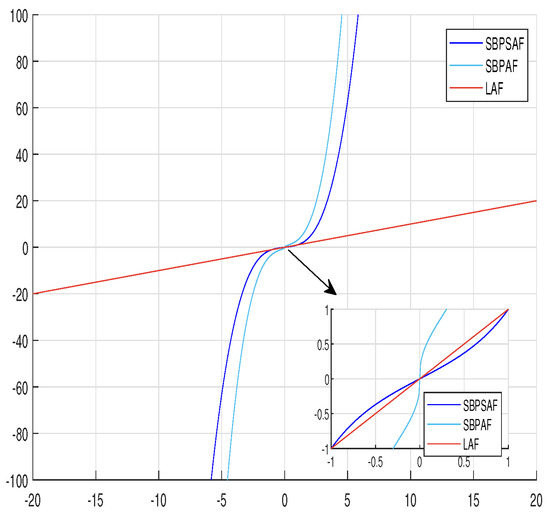
Figure 1. Three sorts of activation functions presented: linear activation function (LAF) ${\Phi }_1$(x) (red solid line), smooth bi-polar sigmoid activation function (SBPSAF) ${\Phi }_2$(x) (sky blue solid line), and signal bi-power activation function (SBPAF) ${\Phi }_3$(x) (blue solid line).

Therefore, in this article, we will use SBPAF as the activation function adopted by ADISZNN.

4. Simulation and Comparative Numerical Experiments

4.1. Comparison Experiments of Activation Functions

In this section, to further validate the correctness of our activation function selection, we compare the ADISZNN models using three different activation functions.

In this example, a two-dimensional dynamic complex matrix $\mathbf{A}$ is presented as follows:

$$\mathbf{A}\left(t\right)=\left[\begin{array}{cc}jsin\left(3t\right)& jcos\left(3t\right)\\ -jcos\left(3t\right)& jsin\left(3t\right)\end{array}\right]\in {\mathbb{C}}^{2\times 2}.$$

(41)

For convenience, this matrix only contains the imaginary part. To verify the correctness of the ADISZNN model, the theoretical inverse of the above dynamic complex matrix is obtained through mathematical calculation:

$${\mathbf{A}}^{-1}\left(t\right)=\left[\begin{array}{cc}-jsin\left(3t\right)& jcos\left(3t\right)\\ -jcos\left(3t\right)& -jsin\left(3t\right)\end{array}\right]\in {\mathbb{C}}^{2\times 2}.$$

(42)

Figure 2 delineates the computational and convergence trajectories of the ADISZNN model across various activation functions, all in the absence of noise. A discernible observation from this figure is that models utilizing the LAF and SBPSAF activation functions achieve near-simultaneous steady-state error close to zero at approximately 2.3 s. In stark contrast, the ADISZNN model equipped with the SBPAF activation function demonstrates a markedly swifter convergence, reaching near-zero error within a mere 0.6 s—a rate that is roughly threefold faster than its counterparts.

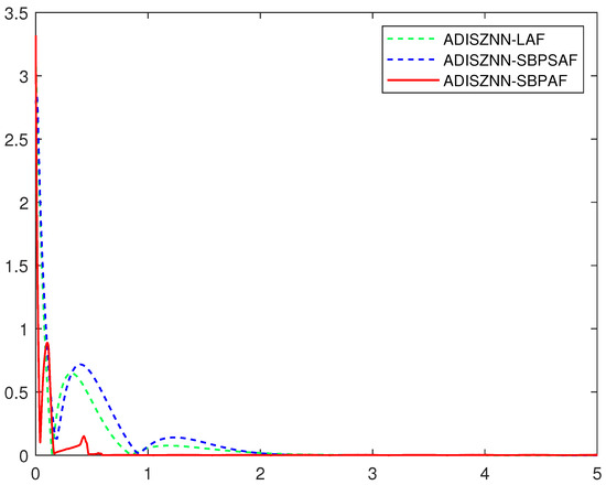
Figure 2. Comparative graph of the computation and convergence processes of ADISZNN with three different activation functions without noise interference; the design parameters are $\lambda =4$ and $\alpha =4$: ADISZNN-LAF (green dashed line), ADISZNN-SBPSAF (blue dashed line), ADISZNN-SBPAF (red solid line).

Figure 3, on the other hand, captures the ADISZNN model’s performance under the influence of linear noise, with each subplot showcasing the model’s behavior when driven by the LAF, SBPSAF, and SBPAF activation functions, respectively. For the readers’ ease, a comparative analysis of these models is tabulated in Table 1. The table underscores a significant finding: the proximity of the activation function’s derivative to the origin is positively correlated with the model’s convergence efficiency. Notably, the ADISZNN model harnessing SBPAF exhibits the most rapid convergence. Nonetheless, it is important to note that models incorporating SBPSAF and SBPAF show a relatively diminished robustness when compared to the LAF-equipped model.

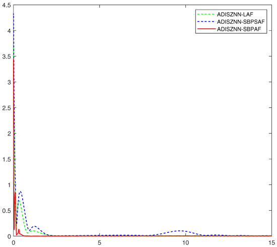
Figure 3. Comparative graph of the computation and convergence processes of ADISZNN with three different activation functions under linear noise $\mathbf{N}={[0.8+4t]}^{2\times 2}$; the design parameters are $\lambda =4$ and $\alpha =4$: ADISZNN-LAF (green dashed line), ADISZNN-SBPSAF (blue dashed line), ADISZNN-SBPAF (red solid line).

Table 1. Comparison of ADISZNN model adopting LAF, SBPSAF, and SBPAF.

AF	LAF	SBPSAF	SBPAF
Derivative near 0 point	Large	Normal	Larger
Convergence	Fast	Normal	Faster
Robustness	Strong	Weak	Normal

These experiments not only confirm the enhanced convergence speed of the ADISZNN model employing the SBPAF activation function proposed in this paper but also validate the appropriateness of the chosen activation function.

Next, we will compare and analyze the convergence performance of the ADISZNN model using the signal bi-power activation function with the DISZNN model without using any activation function under the condition of linear matrix noise interference.

4.2. Comparison Experiments between DISZNN and ADISZNN

The DISZNN model is rewritten as follows:

$$\begin{array}{c}\hfill \dot{\mathbf{E}}\left(t\right)=-s_0^3{\int }_0^t{\int }_0^{\delta }\mathbf{E}\left(\tau \right)d\tau d\delta -3s_0^2{\int }_0^t\mathbf{E}\left(\delta \right)d\delta -3s_0\mathbf{E}\left(t\right)\end{array}$$

(43)

where $s_0\in {\mathbb{R}}^{+}$ is a design parameter.

The error results of the DISZNN model and the ADISZNN model using SBPAF are shown in Figure 4. Under the condition without noise interference, for any initial value of the dynamic complex matrix $\mathbf{X}\left(0\right)\in {[-(2+2j),2+2j]}^{2\times 2}$ the error of the DISZNN model converges almost completely to 0 around 2.8 s. When the SBPAF activation function is introduced, the error of the ADISZNN model converges almost completely to 0 within 0.6 s. Therefore, the convergence speed of the ADISZNN model is significantly faster than that of DISZNN.

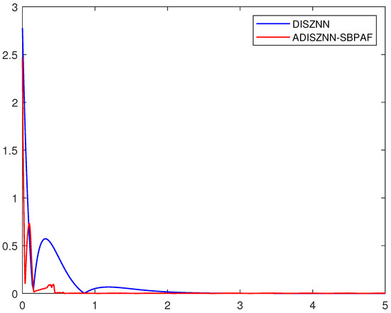
Figure 4. Convergence comparison of ADISZNN and DISZNN without noise interference; the design parameters are $s_0=4$ $\lambda =4$ and $\alpha =4$: ADISZNN-SBPAF (red solid line) and DISZNN (blue solid line).

To compare the tolerance of ADISZNN and DISZNN to noise, a common linear noise $\mathbf{N}={[0.8+4t]}^{2\times 2}$ is introduced. Their numerical experimental comparison is shown in Figure 5, where the design parameters are set as $s_0=4$, $\lambda =4$, and $\alpha =4$. Under the interference of linear noise, both DISZNN and ADISZNN can still make the residual ${\left|\right|\mathbf{E}\left(t\right)\left|\right|}_F$ close to 0 within approximately 2.8 s and 0.6 s, respectively, which is nearly the same as the case without noise interference. This demonstrates that ADISZNN and DISZNN possess inherent tolerance to linear noise.

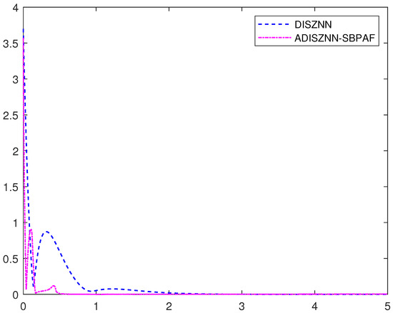
Figure 5. Convergence comparison of ADISZNN and DISZNN, under linear noise $\mathbf{N}={[0.8+4t]}^{2\times 2}$: ADISZNN-SBPAF (pink dotted line) and DISZNN (blue dashed line).

However, during the experimental process, we observed that the residual plot of the ADISZNN model with the signal bi-power activation function exhibits oscillatory fluctuations after reaching the magnitude of ${10}^{-3}$ at 0.6 s. This indicates a decrease in the precision of the model’s computations, as it fails to maintain stable convergence at the ${10}^{-3}$ magnitude level. This implies a reduction in the robustness of the ADISZNN model. The residual plots of the ADISZNN model with noise interference and the comparison of residuals between the DISZNN and ADISZNN models without noise interference are shown in Figure 6 and Figure 7, respectively. In the next subsection, we will discuss the stable version (high-precision version) of the ADISZNN model.

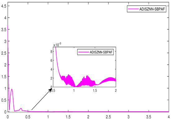
Figure 6. The amplified residual errors of ADISZNN under linear noise $\mathbf{N}={[0.8+4t]}^{2\times 2}$, with design parameters $\alpha =4,\lambda =4,k_1=1,k_2=1,k_3=1,\eta =1/3$, and $omega=3$.

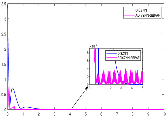
Figure 7. The amplified residual errors of DISZNN and ADISZNN under no noise, with design parameters $\alpha =4,\lambda =4,k_1=1,k_2=1,k_3=1,\eta =1/3,\omega =3$, and $s_0=4$.

4.3. The Stable ADISZNN Model

In this subsection, we propose an improved version of the ADISZNN-SBPAF model to address the oscillation phenomenon (or precision degradation phenomenon). According to the table in experiment 1, we observe that not only can ADISZNN with the signal bi-power activation function accelerate the convergence compared to the DISZNN model, but also the ADISZNN model with the linear activation function (LAF) can similarly accelerate convergence and exhibit stronger robustness.

Based on this observation, we innovatively propose a stable version of the ADISZNN model: When the error of the ADISZNN model using SBPAF approaches zero (i.e., reaches the order of ${10}^{-3}$), we transition the model to use LAF. This transition alters the calculation and convergence of $\left|\right|\mathbf{A}\left(t\right)\mathbf{X}\left(t\right)-{\mathbf{I}\left|\right|}_F$, transforming the ADISZNN-SBPAF model into the ADISZNN-LAF model. The convergence performance of this approach is illustrated in the Figure 8, Figure 9 and Figure 10.

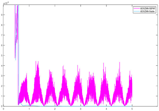
Figure 8. Comparison of the amplified residual errors of stable ADISZNN and unstable ADISZNN under no noise, with design parameters $\alpha =4,\lambda =4,k_1=1,k_2=1,k_3=1,\eta =1/3,\omega =3$, and $s_0=4$.

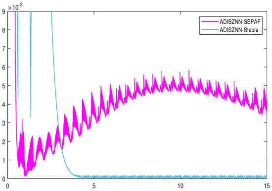
Figure 9. The detailed residual errors of ADISZNN-Stable and ADISZNN-SBPAF, with noise of ${[0.8+4t]}^{2\times 2}$.

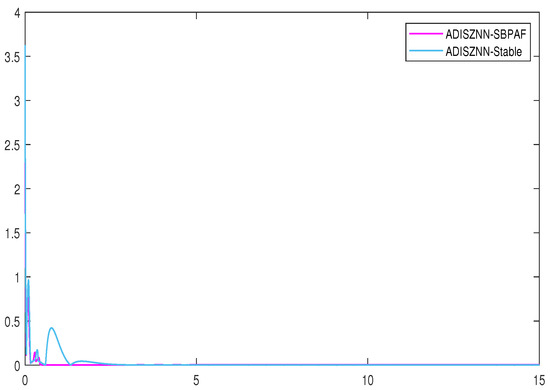
Figure 10. Residual errors of ADISZNN-Stable and ADISZNN-SBPAF with noise of ${[0.8+4t]}^{2\times 2}$.

The residual plots in Figure 9 and Figure 10, respectively, depict the effects of our improvement on the stable version of the ADISZNN model compared to the unstable version (For the reader’s enhanced comprehension, Figure 8 illustrates the comparison of amplified residual errors between the stable and unstable variants of ADISZNN in the absence of noise). While this enhancement results in a slight increase in the convergence time, it strengthens the model’s resistance to noise and improves its robustness. Additionally, the computational accuracy is elevated from the order of ${10}^{-3}$ to ${10}^{-4}$, thereby enhancing the convergence performance of the model.

In Figure 11, a comparison between the stable version of the ADISZNN model and the original DISZNN model is presented. Compared to the original DISZNN model, the stable version of the ADISZNN model exhibits significant improvements. When the computed solution $\mathbf{X}\left(t\right)$ of the model converges to a theoretical state approximation $\mathbf{A}{\left(t\right)}^{-1}$, the convergence time of the stable ADISZNN model is reduced from 2.8 s to 1.9 s. Moreover, the convergence curve of the stable ADISZNN model appears smoother and more refined. Both models achieve a computational accuracy of ${10}^{-4}$ when fully converged. These results indicate that the improved stable version of the ADISZNN model not only enhances the convergence speed but also maintains robustness comparable to that of the DISZNN model.

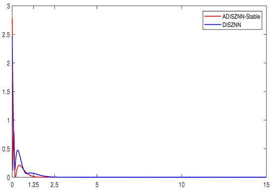
Figure 11. The comparison of the residual errors of stable ADISZNN and DISZNN under linear noise of ${[0.8+4t]}^{2\times 2}$, with design parameters $\alpha =4,\lambda =4,k_1=1,k_2=1,k_3=1,\eta =1/3,\omega =3$, and $s_0=4$.

To underscore the merits of the ADISZNN-Stable model, Figure 12 and Figure 13 depict comparative trajectory plots of the DISZNN alongside the ADISZNN-Stable model under conditions of linear noise. Additionally, Figure 14 presents an analysis of residual errors, contrasting the performance of the DISZNN with that of the ADISZNN-Stable model in an environment devoid of noise.

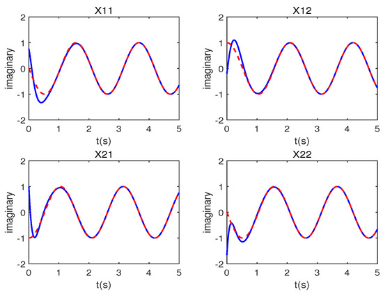
Figure 12. Trajectory analysis for problem (41) under linear noise of ${[0.8+4t]}^{2\times 2}$; the red line points represent the theoretical solution, while the blue line points show the DISZNN model’s solutions.

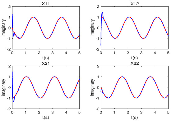
Figure 13. Trajectory analysis for problem (41) under linear noise of ${[0.8+4t]}^{2\times 2}$; the red line points represent the theoretical solution, while the blue line points show the ADISZNN-Stable model’s solutions.

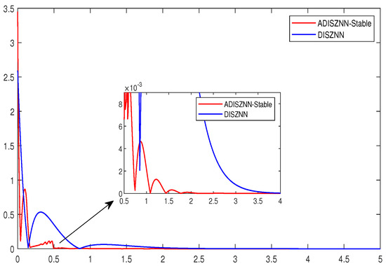
Figure 14. Comparison of the amplified residual errors of stable ADISZNN and DISZNN under no noise, with design parameters $\alpha =4,\lambda =4,k_1=1,k_2=1,k_3=1,\eta =1/3,\omega =3$, and $s_0=4$.

5. Conclusions

This article introduces a novel enhancement to the DISZNN model through the integration of an activation function, culminating in an accelerated dual-integral structure ZNN model. This model exhibits enhanced resilience against linear noise interference, particularly pertinent for dynamic complex matrix inversion challenges. The paper unfolds with the following key contributions: initially, the design formula for a single-integral structure and the DISZNN model are presented and analyzed; subsequently, the architecture of the ADISZNN model is designed, with a theoretical examination of its convergence and robustness; thirdly, both experimental and theoretical analyses are employed to assess the influence of various activation functions on the ADISZNN’s convergence efficacy, thereby substantiating the efficacy of our selected activation function; fourthly, comparative tests under linear noise conditions between the ADISZNN and DISZNN models underscore the ADISZNN’s superior convergence capabilities, albeit with the caveat that the ADISZNN model utilizing the SBPAF activation function exhibits oscillatory behavior, potentially compromising its robustness. In light of these findings, we propose refinements to the ADISZNN-SBPAF model, yielding a more stable iteration of the ADISZNN. Comparative experimentation facilitates the identification of the optimal ZNN configuration. Future inquiries are suggested to investigate the potential applications of the ADISZNN model within the engineering sector. This paper presents the ADISZNN model, which has certain limitations, specifically detailed in Appendix A.

References

- Jin, J.; Chen, W.; Ouyang, A.; Yu, F.; Liu, H. A time-varying fuzzy parameter zeroing neural network for the synchronization of chaotic systems. IEEE Trans. Emerg. Top. Comput. Intell. 2023, 8, 364–376. [Google Scholar] [CrossRef]
- Zhang, R.; Xi, X.; Tian, H.; Wang, Z. Dynamical analysis and finite-time synchronization for a chaotic system with hidden attractor and surface equilibrium. Axioms 2022, 11, 579. [Google Scholar] [CrossRef]
- Rasouli, M.; Zare, A.; Hallaji, M.; Alizadehsani, R. The synchronization of a class of time-delayed chaotic systems using sliding mode control based on a fractional-order nonlinear PID sliding surface and its application in secure communication. Axioms 2022, 11, 738. [Google Scholar] [CrossRef]
- Gao, R. Inverse kinematics solution of Robotics based on neural network algorithms. J. Ambient Intell. Humaniz. Comput. 2020, 11, 6199–6209. [Google Scholar] [CrossRef]
- Hu, Z.; Xiao, L.; Li, K.; Li, K.; Li, J. Performance analysis of nonlinear activated zeroing neural networks for time-varying matrix pseudoinversion with application. Appl. Soft Comput. 2021, 98, 106735. [Google Scholar] [CrossRef]
- Ramos, H.; Monteiro, M.T.T. A new approach based on the Newton’s method to solve systems of nonlinear equations. J. Comput. Appl. Math. 2017, 318, 3–13. [Google Scholar] [CrossRef]
- Andreani, R.; Haeser, G.; Ramos, A.; Silva, P.J. A second-order sequential optimality condition associated to the convergence of optimization algorithms. IMA J. Numer. Anal. 2017, 37, 1902–1929. [Google Scholar]
- Zhang, Y. Revisit the analog computer and gradient-based neural system for matrix inversion. In Proceedings of the 2005 IEEE International Symposium on, Mediterrean Conference on Control and Automation Intelligent Control, Limassol, Cyprus, 27–29 June 2005; IEEE: Piscataway, NJ, USA, 2005; pp. 1411–1416. [Google Scholar]
- Zhang, Y.; Chen, K.; Tan, H.Z. Performance analysis of gradient neural network exploited for online time-varying matrix inversion. IEEE Trans. Autom. Control 2009, 54, 1940–1945. [Google Scholar] [CrossRef]
- Zhang, Y.; Shi, Y.; Chen, K.; Wang, C. Global exponential convergence and stability of gradient-based neural network for online matrix inversion. Appl. Math. Comput. 2009, 215, 1301–1306. [Google Scholar] [CrossRef]
- Xiao, L.; Li, K.; Tan, Z.; Zhang, Z.; Liao, B.; Chen, K.; Jin, L.; Li, S. Nonlinear gradient neural network for solving system of linear equations. Inf. Process. Lett. 2019, 142, 35–40. [Google Scholar] [CrossRef]
- Zhang, Y.; Ge, S. A general recurrent neural network model for time-varying matrix inversion. In Proceedings of the 42nd IEEE International Conference on Decision and Control (IEEE Cat. No. 03CH37475), Maui, HI, USA, 9–12 December 2003; IEEE: Piscataway, NJ, USA, 2003; Volume 6, pp. 6169–6174. [Google Scholar]
- Johnson, M.A.; Moradi, M.H. PID Control; Springer: Heidelberg, Germany, 2005. [Google Scholar]
- Jin, L.; Zhang, Y.; Li, S. Integration-enhanced Zhang neural network for real-time-varying matrix inversion in the presence of various kinds of noises. IEEE Trans. Neural Networks Learn. Syst. 2015, 27, 2615–2627. [Google Scholar] [CrossRef]
- Golub, G.H.; Van Loan, C.F. Matrix Computations; JHU Press: Baltimore, MD, USA, 2013. [Google Scholar]
- Ogata, K. Control systems analysis in state space. In Modern Control Engineering; Pearson Education, Inc.: Hoboken, NJ, USA, 2010; pp. 648–721. [Google Scholar]
- Smith, S. Digital Signal Processing: A Practical Guide for Engineers and Scientists; Newnes: Boston, UK, 2003. [Google Scholar]
- Saleh, B.E.; Teich, M.C. Fundamentals of Photonics; John Wiley & Sons: Hoboken, NJ, USA, 2019. [Google Scholar]
- Trefethen, L.N.; Bau, D. Numerical Linear Algebra; Siam: Philadelphia, PA, USA, 2022; Volume 181. [Google Scholar]
- Zhang, Y.; Li, Z.; Li, K. Complex-valued Zhang neural network for online complex-valued time-varying matrix inversion. Appl. Math. Comput. 2011, 217, 10066–10073. [Google Scholar] [CrossRef]
- Xiao, L.; Zhang, Y.; Zuo, Q.; Dai, J.; Li, J.; Tang, W. A noise-tolerant zeroing neural network for time-dependent complex matrix inversion under various kinds of noises. IEEE Trans. Ind. Inform. 2019, 16, 3757–3766. [Google Scholar] [CrossRef]
- Hua, C.; Cao, X.; Xu, Q.; Liao, B.; Li, S. Dynamic Neural Network Models for Time-Varying Problem Solving: A Survey on Model Structures. IEEE Access 2023, 11, 65991–66008. [Google Scholar] [CrossRef]
- Dai, J.; Jia, L.; Xiao, L. Design and analysis of two prescribed-time and robust ZNN models with application to time-variant Stein matrix equation. IEEE Trans. Neural Netw. Learn. Syst. 2020, 32, 1668–1677. [Google Scholar] [CrossRef]
- Li, S.; Chen, S.; Liu, B. Accelerating a recurrent neural network to finite-time convergence for solving time-varying Sylvester equation by using a sign-bi-power activation function. Neural Process. Lett. 2013, 37, 189–205. [Google Scholar] [CrossRef]
- Lan, X.; Jin, J.; Liu, H. Towards non-linearly activated ZNN model for constrained manipulator trajectory tracking. Front. Phys. 2023, 11, 1159212. [Google Scholar] [CrossRef]
- Liao, B.; Zhang, Y. From different ZFs to different ZNN models accelerated via Li activation functions to finite-time convergence for time-varying matrix pseudoinversion. Neurocomputing 2014, 133, 512–522. [Google Scholar] [CrossRef]
- Xiao, L. A nonlinearly activated neural dynamics and its finite-time solution to time-varying nonlinear equation. Neurocomputing 2016, 173, 1983–1988. [Google Scholar] [CrossRef]
- Yang, Y.; Zhang, Y. Superior robustness of power-sum activation functions in Zhang neural networks for time-varying quadratic programs perturbed with large implementation errors. Neural Comput. Appl. 2013, 22, 175–185. [Google Scholar] [CrossRef]
- Liao, B.; Zhang, Y. Different complex ZFs leading to different complex ZNN models for time-varying complex generalized inverse matrices. IEEE Trans. Neural Netw. Learn. Syst. 2013, 25, 1621–1631. [Google Scholar] [CrossRef]
- Xiao, L.; Tan, H.; Jia, L.; Dai, J.; Zhang, Y. New error function designs for finite-time ZNN models with application to dynamic matrix inversion. Neurocomputing 2020, 402, 395–408. [Google Scholar] [CrossRef]
- Lv, X.; Xiao, L.; Tan, Z.; Yang, Z. Wsbp function activated Zhang dynamic with finite-time convergence applied to Lyapunov equation. Neurocomputing 2018, 314, 310–315. [Google Scholar] [CrossRef]
- Li, Z.; Liao, B.; Xu, F.; Guo, D. A New Repetitive Motion Planning Scheme With Noise Suppression Capability for Redundant Robot Manipulators. IEEE Trans. Syst. Man Cybern. Syst. 2020, 50, 5244–5254. [Google Scholar] [CrossRef]
- Liao, B.; Han, L.; Cao, X.; Li, S.; Li, J. Double integral-enhanced Zeroing neural network with linear noise rejection for time-varying matrix inverse. CAAI Trans. Intell. Technol. 2023, 9, 197–210. [Google Scholar] [CrossRef]
- Zhang, M. A varying-gain ZNN model with fixed-time convergence and noise-tolerant performance for time-varying linear equation and inequality systems. Authorea Prepr. 2023. Available online: https://www.techrxiv.org/doi/full/10.36227/techrxiv.16988404.v1 (accessed on 4 April 2024).
- Zhang, Z.; Deng, X.; Qu, X.; Liao, B.; Kong, L.D.; Li, L. A varying-gain recurrent neural network and its application to solving online time-varying matrix equation. IEEE Access 2018, 6, 77940–77952. [Google Scholar] [CrossRef]
- Han, L.; Liao, B.; He, Y.; Xiao, X. Dual noise-suppressed ZNN with predefined-time convergence and its application in matrix inversion. In Proceedings of the 2021 11th International Conference on Intelligent Control and Information Processing (ICICIP), Dali, China, 3–7 December 2021; IEEE: Piscataway, NJ, USA, 2021; pp. 410–415. [Google Scholar]
Disclaimer/Publisher’s Note: The statements, opinions and data contained in all publications are solely those of the individual author(s) and contributor(s) and not of MDPI and/or the editor(s). MDPI and/or the editor(s) disclaim responsibility for any injury to people or property resulting from any ideas, methods, instructions or products referred to in the content. |
© 2024 by the authors. Licensee MDPI, Basel, Switzerland. This article is an open access article distributed under the terms and conditions of the Creative Commons Attribution (CC BY) license (https://creativecommons.org/licenses/by/4.0/).