Abstract
It is generally known that in order to solve the split equality fixed-point problem (SEFPP), it is necessary to compute the norm of bounded and linear operators, which is a challenging task in real life. To address this issue, we studied the SEFPP involving a class of quasi-pseudocontractive mappings in Hilbert spaces and constructed novel algorithms in this regard, and we proved the algorithms’ convergences both with and without prior knowledge of the operator norm for bounded and linear mappings. Additionally, we gave applications and numerical examples of our findings. A variety of well-known discoveries revealed in the literature are generalized by the findings presented in this work.
Keywords:
fixed-point problem; iterative algorithm; quasi-pseudocontractive mapping; weak and strong convergences MSC:
47H09; 47H10; 47J25
1. Introduction
In this manuscript, we utilize the following notations: denotes an inner product and represents its corresponding norm. We designate as Hilbert spaces, as nonempty, convex, and closed subsets of and as bounded and linear mappings. The symbols ⇀ and → signify weak and strong convergences, respectively.
A mapping is known as a fixed point of (Fix()) if for all We denote the set of Fix() by . is known to be quasi-nonexpansive if It is obvious that if is quasi-nonexpansive then is called demicontractive if and and it is called quasi-pseudocontractive if is known as strongly monotone if
Remark 1.
The quasi-pseudocontractive mapping encompasses various types of mappings, including quasi-nonexpansive, demicontractive, and several others. For further details, please refer to [1] and the cited references therein.
The problem of finding
is known as the “Split Feasibility Problem (SFP)”. The SFP, initially introduced by [2], has garnered significant attention from researchers due to its versatile applications in practical domains. These applications span a wide spectrum, encompassing fields such as signal processing, intensity-modulated radiation therapy, and image reconstruction, as documented in [3,4,5].
If the problem stated in (1) possesses a solution, it is evident that is a solution to Equation (1) if and only if it also solves
where are metric projections on respectively.
To address problem (1), Byrne [6] proposed the following algorithm, known as the CQ algorithm:
where Equation (3) involves the computation of onto and this is known to be implementable when the projections have closed-form expressions.
Related to SFP, we have the “Split Equality Problem (SEP)”. This problem was introduced by Moudafi and Al-Shemas [7] and it entails finding
By using (identity mapping), it is easy to see that the SEP reduces to the SFP. The following algorithm was taken into consideration by Moudafi and Al-Shemas [7] to solve the SEP (4):
where are chosen arbitrarily and were metric projections on After some certain condition was imposed on they obtained a weak convergence result.
As any nonempty, closed, and convex subset of a Hilbert space can be viewed as the fixed point set of its corresponding projector, Equation (4) is consequently simplified to find
where are nonlinear operators with Equation (6) is regarded as the “Split Equality Fixed-Point Problem (SEFPP)”.
Motivated by the result in [7], Moudafi [8] considered the algorithm below:
After some conditions were imposed on the parameters and operators involved, they proved weak convergence results.
To solve (7), the inverse of a bounded and linear operator must be computed, and this is known to be no easy task. This is why Byne [6] considered an algorithm for solving the SFP without the stated inverse.
It was reported by Mohammed and Kilicman [9] that the SFP can be reduced to a convex feasibility problem (CFP) as well as a fixed-point problem (FPP). Fixed-point theory (FPT) can be considered a core area of research in nonlinear analysis due to its various applications in many areas of research, such as image processing and equilibrium problems, the study of the existence and uniqueness of solutions for the integral, and differential equations, selection, and matching problems (see Mohammed et al. [10]).
The roots of fixed-point theory can be traced back to the early developments in topology, notably through contributions from Poincaré, Lefschetz–Hopf, and Leray–Schauder. These pioneers laid the groundwork that now spans diverse areas of analysis. Topological considerations play a pivotal role in FPT, often intersecting with degree theory to tackle significant existence problems. This approach is invaluable in scenarios ranging from solving elliptic partial differential equations to identifying closed periodic orbits in dynamical systems. For more details, see Khan [11]. For further exploration, recent studies by Antón-Sancho [12] delve into the fixed points of automorphisms within vector bundle moduli spaces over compact Riemann surfaces, offering new perspectives and advancing the interdisciplinary scope of fixed-point theory.
Moudafi’s algorithm in [8] involved firmly quasi-nonexpansive mapping; this mapping includes the quasi-nonexpansive class. Very recently, Che and Li [13] considered the following algorithm for finding the solution of the SEP and proved the convergence results of the algorithm:
where and are strictly pseudononspreading mappings.
Since quasi-pseudocontractive mapping includes firmly quasi-nonexpansive, quasi-nonexansive, directed, and demicontractive mappings, this motivated Chang et al. [1] to introduce the following algorithm for solving the SEFPP involving quasi-pseudocontractive mappings and proved the convergence result of the algorithm:
The proposed algorithm by Chang et al. [1] requires prior knowledge of operator norms. A similar result had been proved in [14]. Very recently, Mohammed et al. [10] proved the convergence of the following algorithm for the class of total quasi-asymptotically nonexpansive mappings:
The findings in [1,10,14] both converged weakly; in an infinite-dimensional space, weak convergence does not imply strong convergence, whereas strong and weak convergences coincide if the dimension is finite.
Based on these findings, we set out to develop new methods for solving the SEFPP for quasi-pseudocontractive mappings in Hilbert spaces and to demonstrate how the suggested methods converge. The suggested algorithms’ convergence findings will also be presented in a form that frees them from the constraints imposed by the operator norm of bounded and linear operators. At the end, we provide numerical examples that highlight our findings.
2. Preliminaries
This section offers a few fundamental findings that support the paper’s primary findings.
Definition 1.
A mapping is said to be semi-compact if for any bounded sequence with then there exist such that
Lemma 1
(Chang et al. [14]). Suppose is Lipschitz with and then
- a.
- b.
- is demiclosed at zero only if is demiclosed at zero.
- c.
- is Lipschitz with
- d.
- is quasi-nonexpansive only if is quasi-pseudocontractive.
Lemma 2
(Opial, [15]). Suppose for then
- a.
- , exist;
- b.
- For any weak cluster point of then
Lemma 3
(Xu, [16]). Let such that
where then
- a.
- b.
- then,
Lemma 4
(Xu, [16]). Let such that If
then exist.
3. Main Results
The sequel will use to represent the solution set for (6), that is
The following presumptions were used to approximate (11).
Suppose that
- (A1)
- are two quasi-pseudocontractive operators with in addition, suppose is L-Lipschitz.
- (A2)
- are linear and bounded operators with their adjoints and respectively.
- (A3)
- are demiclosed at origin.
- (A4)
- Let and be defined below:where
- (A5)
- Algorithm:Let ( be defined bywhere are chosen arbitrarily, and where and , respectively,
Theorem 1.
Suppose – are held and that Then, defined by (13) converges weakly to in addition if and are semi-compact, then converges strongly to
Proof.
Similarly,
This implies that
where
Thus, therefore, is a decreasing sequence that is bound from below by 0, hence, converges, therefore, we have that
These lead to
Since, , where and is Lipschitz, we have
Therefore,
Similarly,
Since converges, it follows that is bounded, which implies that there exist for which and
On the other hand, and together with
we deduce that Similarly, These imply that and see Lemma 1.
Now that and couple with the demiclosedness of at origin, we have
Similarly, and together with the demiclosedness of at origin, we see that
Since and and are linear mappings, we have
This implies that
which implies that
Therefore, Noticing that , we conclude that
Thus,
- (i)
- exist, for all
- (ii)
- belong to
Hence, by Lemma 2, we see that Furthermore, since is bounded coupled with Equation (24) and Definition 1 we deduce that This completes the proof. □
4. The SEFPP without Prior Knowledge of Operator Norms
This section gives the convergent result of the SEFPP without prior knowledge of the operator norms of bounded and linear operators and respectively.
Theorem 2.
Assume – are satisfied, , and let be defined by
where are chosen arbitrarily and
- (i)
- (ii)
- such that and
then, In addition, if and are semi-compact, then
Proof.
Similarly,
where and
where is quasi-nonexpansive. By (27) and (29), and the fact that we have
where and
The fact that is -Lipschitzian, we have
This gives
Similarly,
This gives
where
Noticing that by Lemma 4 we deduce that exist. Thus, is bounded, and it is not difficult to see that is bounded.
Next, we show that and
Since and is bounded, thus, we deduce from (38) that
On the other hand,
and
Similarly,
By (44), we deduce that
On the other hand,
Noticing that thus, by Lemma 4, we deduce that
It is known that is quasi-nonexpansive mapping if and only if This implies that
Thus, by (49) we get
Similarly,
and
Next, we show that This follows directly from Section 3. This completes the proof. □
Corollary 1.
Suppose for are demicontractive mappings with such that are demiclosed at zero. Let be generated by
where are chosen arbitrarily, and where and respectively. Then, defined by (55) converges to
Corollary 2
(Chang et al. [14]). Suppose – are satisfied, and that Let defined by
where and with and are chosen arbitrarily. Then, converges to
Proof.
Corollary 3
(Chang et al. [1]). Suppose – are satisfied and that Let defined by
where and with and are chosen arbitrarily. Then, converges to
5. Applications
This section provides applications for SEFPP.
5.1. Application to the SFP
We denote the solution set of the SFP (1) by
In (4), if (identity mapping), then the SEFPP reduces to (1). Furthermore, in algorithm (13), let we therefore deduce the following result:
Corollary 4.
Let and be as in Theorem 1. Let be defined by
where and with and are chosen arbitrarily. Then, converges weakly to
5.2. Application to the Split Variational Inequality Problem (SVIP)
The SVIP was introduced by Censor et al. [17] and it entails finding
where are some nonlinear mappings.
Equation (59) is called the variational inequality problem (VIP), and we denote its solution set by Subsequently, the solution set of the SVIP is denoted by
Let be defined by
and be defined by
For the re-solvent operators of and are denoted by and , and are defined by
and
respectively.
It was proved in [1] that and are quasi-pseudocontractive and 1-Lipschitzian mappings with and Therefore, the SVIP is equivalent to the following split equality fixed-point problem:
Hence, we have the following result: Suppose that
- (B1)
- (B2)
- and as in Theorem 1.
- (B3)
- and are demiclosed at zero.
- (B4)
- Let and be defined as follows:where
- (B5)
- Algorithm:Let be defined bywhere are chosen arbitrarily, and with and respectively.
Corollary 5.
Suppose that assumptions are satisfied and that Then, the sequence generated by (65) converges to the solution of SVIP.
5.3. Application to the Split Convex Minimization Problem (SCMP)
Let and be lower semi-continuous and proper convex functions. The SCMP is formulated as follows:
We denote the solution set of the SCMP by
Let and be defined by and respectively. For arbitrary Chang et al. [1] defined the re-solvent operators of h and l as follows:
and
It was proved in [1] that and Therefore, the SCMP for and is equivalent to the following SEFPP:
It was proved in [1] that and are firmly nonexpansive with and hence, we deduce the following results from Theorem 1: Suppose that
- (C1)
- and be defined as above;
- (C2)
- and as in Theorem 1;
- (C3)
- and are demiclosed at zero;
- (C4)
- Let and be defined aswhere
- (C5)
- Algorithm: Let be defined aswhere and are chosen arbitrarily, and where and respectively.
Corollary 6.
Suppose that assumptions are satisfied and that Then, the sequence generated by (69) converges weakly to the solution of the SCMP.
6. Numerical Examples
This section gives numerical examples that illustrate our results.
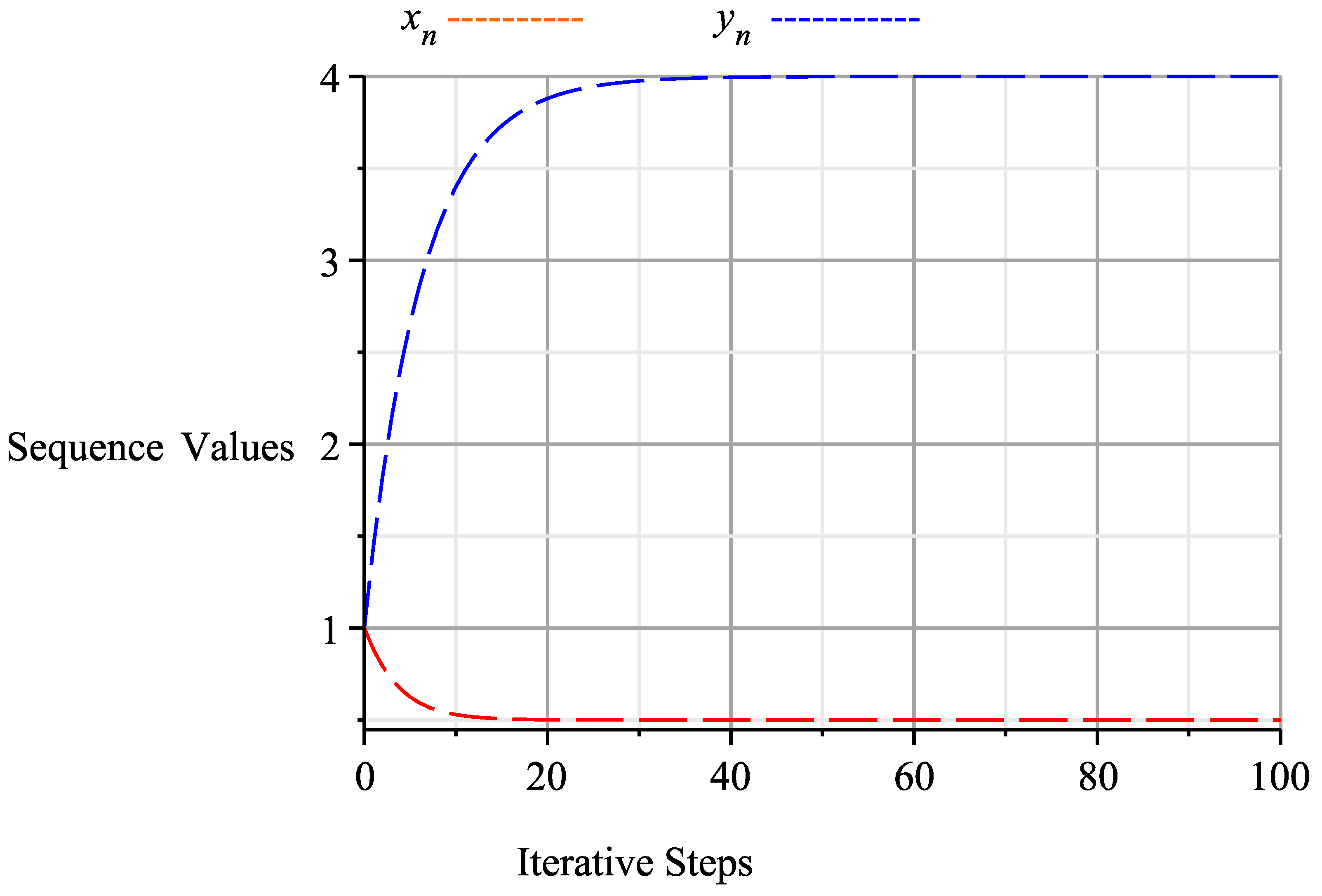
Example 1.


In Theorem 1, let and let , then and . Define and by and , for all Clearly, T and S are quasi-pseudo-demicontractive mappings with Fix(T) = 4 and Fix(S) = , and (I-T) and (I-S) are demiclosed at zero. In algorithm (11), let clearly, these parameters satisfy the hypothesis of Theorem 1. Setting the number of iterations to 100 by using Maple, we obtain the following results in Table 1 and Figure 1:
Table 1.
Numerical results of algorithm (13) starting with the initial values and which shows that converges to (4, 1/2).
Figure 1.
Graph of algorithm (13) at 100 iterations, starting with the initial values and which shows that converges to (4, 1/2).
Example 2.
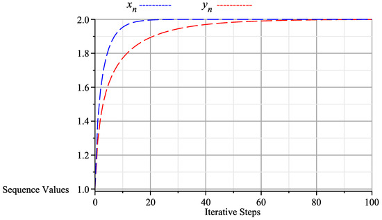
In Theorem 1, let and let , then and . Define and by
and , for all Clearly, T and S are quasi-pseudo-demicontractive mappings with Fix(T) = 2 and Fix(S) = 2, and (I-T) and (I-S) are demiclosed at zero. In algorithm (13), choose . Clearly, these parameters satisfy the hypothesis of Theorem (1). Setting the number of iterations to 1000 by using Maple, we obtain the following results in Table 2 and Figure 2:
Table 2.
Numerical results of algorithm (13) starting with the initial values and which shows that converges to (2,2).
Figure 2.
Graph of algorithm (13) at 100 iterations, starting with the initial values and which shows that converges to (2,2).
7. Conclusions
It is generally known that in order to solve the split equality fixed-point problem (SEFPP), it is necessary to compute the norm of bounded and linear operators, which is a challenging task in real life. To address this issue, we studied the SEFPP involving the class of quasi-pseudocontractive mappings in Hilbert spaces and constructed novel algorithms in this regard, and we proved the algorithms’ convergences both with and without prior knowledge of the operator norm for bounded and linear mappings. Additionally, we gave applications and numerical examples of our findings as discussed in the Table 1 and Table 2 and graphs in Figure 1 and Figure 2, respectively. The discoveries highlighted in this work contribute to the generalization of various well-known findings documented in the literature. Furthermore, quasi-pseudocontractive mappings encompass various types, including quasi-nonexpansive, demicontractive, and directed mappings.
The SEFPP explored in our study is highly general; as a special example, it covers a wide range of problems, including split fixed points, split equality, and split feasibility problems. Our findings not only complement and generalize the findings in Chang et al. [1], Moudafi [7,8], and Chang et al. [14], but also offer a cohesive framework for researching further problems pertaining to the SEFPP.
Finally, strong convergence was obtained by imposing the semi-compactness condition. This compactness condition appears very strong as some mappings are not semi-compact; therefore, new research can be carried out to prove the strong convergence results without imposing the compactness condition.
Author Contributions
All authors contributed equally and have reviewed and approved the final version of the manuscript for publication.
Funding
This research did not receive any external funding.
Data Availability Statement
No new data were created or analyzed in this study.
Conflicts of Interest
The authors have disclosed that they have no conflicts of interest.
References
- Chang, S.-S.; Yao, J.-C.; Wen, C.-F.; Zhao, L.-C. On the split equality fixed point problem of quasi-pseudo-contractive mappings without a priori knowledge of operator norms with applications. J. Optim. Theory Appl. 2020, 185, 343–360. [Google Scholar] [CrossRef]
- Censor, Y.; Elfving, T. A multiprojection algorithm using Bregman projections in a product space. Numer. Algorithms 1994, 8, 221–239. [Google Scholar] [CrossRef]
- Censor, Y.; Bortfeld, T.; Martin, B.; Trofimov, A. A unified approach for inversion problems in intensity-modulated radiation therapy. Phys. Med. Biol. 2006, 51, 2353–2365. [Google Scholar] [CrossRef] [PubMed]
- Censor, Y.; Elfving, T.; Kopf, N.; Bortfeld, T. The multiple-sets split feasibility problem and its applications for inverse problems. Inverse Probl. 2005, 21, 2071–2084. [Google Scholar] [CrossRef]
- Censor, Y.; Motova, A.; Segal, A. Perturbed projections and subgradient projections for the multiple-sets split feasibility problem. J. Math. Anal. Appl. 2007, 327, 1244–1256. [Google Scholar] [CrossRef]
- Byrne, C. Iterative oblique projection onto convex subsets and the split feasibility problem. Inverse Probl. 2002, 18, 441–453. [Google Scholar] [CrossRef]
- Moudafi, A.; Al-Shemas, E. Simultaneous iterative methods for split equality problem. Trans. Math. Program. Appl. 2013, 1, 1–10. [Google Scholar]
- Moudafi, A. Alternating CQ-algorithm for convex feasibility and split fixed-point problems. J. Nonlinear Convex Anal. 2014, 15, 809–818. [Google Scholar]
- Mohammed, L.B.; Kılıçman, A. Strong Convergence for the Split Common Fixed-Point Problem for Total Quasi-Asymptotically Nonexpansive Mappings in Hilbert Space. Abstr. Appl. Anal. 2015, 2015, 1–7. [Google Scholar] [CrossRef]
- Mohammed, L.; Kılıçman, A.; Saje, A.U. On split equality fixed-point problems. Alex. Eng. J. 2023, 66, 43–51. [Google Scholar] [CrossRef]
- Khan, A.R. Iterative Methods for Nonexpansive Type Mappings. In Fixed Point Theory and Graph Theory; Academic Press: Cambridge, MA, USA, 2016; pp. 231–285. [Google Scholar]
- Antón-Sancho, Á. Fixed points of automorphisms of the vector bundle moduli space over a compact Riemann surface. Mediterr. J. Math. 2024, 21, 1–20. [Google Scholar] [CrossRef]
- Che, H.; Li, M. A simultaneous iterative method for split equality problems of two finite families of strictly pseudononspreading mappings without prior knowledge of operator norms. Fixed Point Theory Appl. 2015, 2015, 1. [Google Scholar] [CrossRef]
- Chang, S.-S.; Wang, L.; Qin, L.-J. Split equality fixed point problem for quasi-pseudo-contractive mappings with applications. Fixed Point Theory Appl. 2015, 2015, 208. [Google Scholar] [CrossRef]
- Opial, Z. Weak convergence of the sequence of successive approximations for nonexpansive mappings. Bull. Am. Math. Soc. 1967, 73, 591–597. [Google Scholar] [CrossRef]
- Xu, H.-K. Iterative Algorithms for Nonlinear Operators. J. Lond. Math. Soc. 2002, 66, 240–256. [Google Scholar] [CrossRef]
- Censor, Y.; Gibali, A.; Reich, S. Algorithms for the Split Variational Inequality Problem. Numer. Algorithms 2012, 59, 301–323. [Google Scholar] [CrossRef]

Disclaimer/Publisher’s Note: The statements, opinions and data contained in all publications are solely those of the individual author(s) and contributor(s) and not of MDPI and/or the editor(s). MDPI and/or the editor(s) disclaim responsibility for any injury to people or property resulting from any ideas, methods, instructions or products referred to in the content. |
© 2024 by the authors. Licensee MDPI, Basel, Switzerland. This article is an open access article distributed under the terms and conditions of the Creative Commons Attribution (CC BY) license (https://creativecommons.org/licenses/by/4.0/).