Abstract
A kind of reduced-dimension method based on a weighted explicit finite difference scheme and the proper orthogonal decomposition (POD) technique for diffusion equations with Riemann–Liouville fractional derivatives in space are discussed. The constructed approximation method written in matrix form can not only ensure a sufficient accuracy order but also reduce the degrees of freedom, decrease storage requirements, and accelerate the computation rate. Uniqueness, stabilization, and error estimation are demonstrated by matrix analysis. The procedural steps of the POD algorithm, which reduces dimensionality, are outlined. Numerical simulations to assess the viability and effectiveness of the reduced-dimension weighted explicit finite difference method are given. A comparison between the reduced-dimension method and the classical weighted explicit finite difference scheme is presented, including the error in the norm, the accuracy order, and the CPU time.
Keywords:
weighted explicit finite difference scheme; space-fractional diffusion equation; reduced-dimension weighted explicit finite difference scheme; proper orthogonal decomposition method; uniqueness; stabilization; error estimation MSC:
65M06
1. Introduction
The initial boundary value problems addressed here are as follows:
where represents the diffusion coefficient, T is the final time, and denotes the source term. is the initial value, which is sufficiently smooth. The term is used to represent the Riemann–Liouville fractional derivative, which has the following definition:
in which represents the order of the equation, and (see [1,2]).
Fractional calculus emerges as an indispensable mathematical instrument for elucidating a spectrum of phenomena encountered in scientific and engineering disciplines [3,4,5,6,7]. Within this versatile framework, one of the key applications is the depiction of subdiffusion and superdiffusion [8,9,10]. The fractional diffusion equation’s importance and use in various fields have garnered significant interest. However, the complexity of fractional diffusion equations typically makes it difficult to obtain solutions that are precisely accurate. Consequently, it becomes necessary for us to utilize numerical approaches to obtain numerical solutions to these equations. As we know, there exist challenges in the numerical approximation of fractional derivatives because of their lack of the advantageous properties that classical approximation operators possess. So, many researchers keep working hard on constructing approximate formulas for fractional derivatives. And, during the preceding decades, there has been notable progress, for example, the finite difference method [1,2,11,12]. Utilizing the traditional Grünwald–Letnikov technique for discretizing the Riemann–Liouville fractional derivative [3], first-order accuracy was obtained; however, the technique is unstable in time-dependent contexts. Meerschaert and Tadjeran [1] proposed the shifted Grünwald–Letnikov formula to approximate the fractional advection–dispersion flow equation, ensuring stability. Wang et al. [13] approximated the space-fractional diffusion equation by weighting the Grünwald–Letnikov formula and shifting Grünwald–Letnikov formula. Savović et al. [14] studied radon diffusion in soil and air, deriving the solution of the correlation diffusion equation using the explicit finite difference method. They compared the results of the two-medium model (soil–air) with those of the simplified single-medium model (soil). Savović et al. [15] used the explicit finite difference method (EFDM) and a physical information neural network (PINN) to study Burgers’ equation. Although the method above performs well, it contains too many degrees of freedom for practical calculations. Therefore, a significant problem is how to simplify computations, reduce computational and storage requirements, and slow the accumulation of truncation errors during the calculation process, all while ensuring that the numerical solution maintains sufficient precision. A possible solution to achieve these goals is to construct a kind of reduced-dimension method.
A wealth of numerical evidence demonstrates the efficacy of the POD technique as a potential and practical reduced-dimension method that can reduce the unknowns of the numerical models, slow down the accumulation of round-off errors, minimize CPU running time, and enhance computational efficiency to some extent [16,17,18]. The POD method has been applied in many fields, including but not limited to turbulence analysis [19,20,21], principal component analysis [22], sample identification for statistics [23], atmospheric modeling [24], geophysics [25], and so on. In particular, the POD dimension reduction technique is commonly integrated with many classical numerical methods to develop different reduced-dimension models, including POD finite volume element models [26], the mixed finite element method based on the POD technique [27,28], the space–time POD element method [29,30], reduced-dimension spectral methods [31,32], and difference methods combined with the POD method [33,34,35,36], etc. These reduced-dimension schemes have achieved a lot of meaningful results.
However, to our knowledge, there have been no reports about a reduced-dimension weighted finite difference scheme for the space-fractional diffusion equation established by the POD method. Therefore, this is our main purpose in this paper. To achieve this, we have developed a reduced-dimension model for space-fractional diffusion equations by combining the weighted finite difference scheme and the POD method. The weighted explicit finite difference form is given and written in matrix form. Additionally, the uniqueness of the solution with this method is proven. Based on the classical difference method with the matrix form, a reduced-dimension weighted explicit finite difference method is obtained by selecting suitable samples, establishing a snapshot matrix, and constructing a POD basis. Uniqueness, stability, and error estimations are presented through matrix analysis. Numerical simulations for assessing the viability and efficiency of the reduced-dimension weighted explicit finite difference method are provided. A comparison between the reduced-dimension method and the classical weighted explicit finite difference scheme is presented, including the error in the norm, the accuracy order, and the CPU time. The results demonstrate that the POD reduced-dimension weighted explicit finite difference scheme can ensure precision while saving CPU computation time and improving computing efficiency.
The paper is structured as follows. In Section 2, we present a matrix formulation of the weighted explicit finite difference scheme for the space-fractional diffusion equation and demonstrate the uniqueness of its solutions. Furthermore, Section 3 describes the creation of POD bases and the establishment of a reduced-dimension weighted explicit finite difference scheme using POD techniques. In Section 4, the uniqueness, stabilization, and error estimates of the reduced-dimension weighted explicit finite difference solutions are provided, and the implementation steps of the POD reduced-dimension method are described. For the purpose of verifying the constructed scheme’s efficiency and feasibility, numerical simulations are presented in Section 5. Finally, Section 6 provides the main conclusions.
2. The Weighted Explicit Finite Difference Scheme for the Space-Fractional Diffusion Equation
To establish the weighted explicit finite difference scheme for problem (1), the discretized space and time variables are given. The time is divided as . Let denote the time step, . And, let be space mesh nodes, with the equivalent step length , and for .
We define the grid function as
Before constructing the weighted explicit finite difference method, we first define the Grünwald–Letnikov formula for :
Next, we define the right-shifted Grünwald–Letnikov formula for [1]:
where M is a positive integer, and denotes the Gamma function [3] defined by the integral.
We rewrite Equations (2) and (3) as follows, respectively:
The ‘normalized’ Grünwald weight is defined by
in which represents a binomial coefficient.
The coefficient , which is the coefficient of the power series of the function , is determined by just the order and the index k:
The following is their recurrence relationship:
Lemma 1
([37]). When , the coefficient in Equation (6) satisfies the properties below:
The following difference quotient can be applied to approximate the derivative of (1):
By combining Equations (4) and (5), we obtain the finite difference equation as follows:
Equations (9) and (10) possess only first-order precision in both time and space [1]. To achieve higher precision in space, we can employ a weighted approach with the Grünwald–Letnikov formula and the right-shifted Grünwald–Letnikov formula:
Therefore, the weighted explicit finite difference scheme for initial boundary value problems (1) can be obtained:
in which is a weight parameter. In this article, we take the weight parameter as .
Let be defined as with the condition that . Equation (12) can then be rewritten as follows:
Furthermore, the matrix form of the weighted explicit finite difference scheme (13) can be rewritten as follows:
in which the factor
The element in matrix for and are defined as follows (note that the values of and are given in Lemma 1):
Theorem 1.
The weighted explicit finite difference scheme (12) has a unique solution.
Proof of Theorem 1.
Assuming that is another solution of Equation (12) and defining , we obtain
Let , where . In the above equation, setting , taking the absolute value on both sides and then applying the triangle inequality, we obtain the following result:
For , Equation (18) can be written as follows:
Similarly, for , we obtain
and by the principle of induction, we obtain
Due to , the equation can be rewritten as follows:
where .
Owing to , it follows that , which implies . Consequently, the finite difference scheme (12) has a unique solution, thereby proving the conclusion of Theorem 1. □
The stabilization and convergence of the set of solutions were proved in Theorems 2.2 and 2.3, as referenced in [13].
Theorem 2.
Given and the condition , the series of solutions for the weighted explicit finite difference scheme (14) is stabilized and converges. Furthermore, the error estimates between this series and the analytical solution vector for , produced by the space-fractional diffusion Equation (1), are denoted as follows.
Remark 1.
The series of solutions for the weighted explicit finite difference scheme can be obtained in vector format by providing the space step h, time step τ, coefficients , initial values , and parameters ϵ. From this series, we select the first S as a group of snapshots.
3. The Establishment of a Reduced-Dimension Scheme for the Space-Fractional Diffusion Equation
As we know, the matrix is , and there are unknowns in Equation (14) when solving the equations obtained from the weighted explicit finite difference scheme. When M is larger, it can significantly limit the computation speed in practical implementation. To enhance the efficiency of computation and simplify the procedure, in this section, we construct a reduced-dimension model of the weighted explicit finite difference scheme based on the POD method.
3.1. Construction of POD Base
Firstly, we compute the first solution vectors , in the weighted explicit finite difference scheme as snapshots. Then, we establish an snapshot matrix :
Subsequently, the snapshot matrix undergoes factorization via the technique of singular value decomposition, that is,
in which the diagonal matrix is made up of the singular values of sorted in descending order, that is, . Matrix is an orthogonal matrix whose column vectors are the orthonormal eigenvectors corresponding to . Similarly, matrix , which is an orthogonal matrix, is defined as . The column vectors of matrix are the orthonormal eigenvectors that correspond to . The symbol denotes the zero vector [17].
Take
where the diagonal matrix is , which is made up of the diagonal matrix in ’s first q positive singular values.
Lemma 2.
Let be composed of ’s first q eigenvectors. Then, it holds that
The proof of Lemma 2 has been shown in Lemma 1.2.2 of reference [17].
Consequently, based on the relationship between matrix norms and the spectral radius [38], it follows that
where .
Moreover, assuming that the S column vector of is represented by , (), the following results are obtained:
In this context, denotes the projection of onto , represents the inner product between and , and is an S-dimensional unit vector with the nth component 1 (). Inequality indicates that the error between and is no greater than . Consequently, represents the best approximation of , and constitutes the optimal POD basis for .
Remark 2.
The S order of matrix is significantly smaller than the order of matrix , indicating that the number of snapshots S is far less than the number of space nodes . However, their positive eigenvalues () are identical. Therefore, we calculate the first q positive eigenvalues (for ) and the corresponding eigenvectors (for ) of matrix . Then, utilizing the formula (for ), we compute the positive eigenvalues (for ) of matrix , which corresponds to the eigenvectors (for ). By doing so, we gain access to a set of POD bases (with , typically choosing ).
3.2. The Establishment of the Reduced-Dimension Scheme Based on POD
The first reduced-dimension weighted explicit finite difference solutions, , are found in Section 3.1, where and . And, we replace in Equation with and . Then, we can obtain the reduced-dimension weighted explicit finite difference scheme for the space-fractional diffusion equation as follows:
in which is the solution coefficient vectors for the first S columns of Equation (14). The definition of matrix is given in Equations (15) and (16). We multiply both sides of Equation (26) by . Based on the orthonormality of the POD bases, we obtain the reduced-dimension weighted explicit finite difference scheme of unknown vectors as follows:
Remark 3.
It is observed that scheme (14) contains unknowns at each time node, whereas scheme (27) has only q unknowns at the same time node . As a result, we can see that the reduced-dimension weighted explicit finite difference scheme (27) contains very few degrees of freedom, considerably reduces the CPU running time, and delays the accumulation of computation errors.
4. The Uniqueness, Stabilization, and Error Estimates for the Reduced-Dimension Weighted Explicit Finite Difference Solutions and the Algorithmic Process of the POD Technique
4.1. The Uniqueness, Stabilization, and Error Estimates for the Reduced-Dimension Weighted Explicit Finite Difference Solutions
Before providing the error estimates for the reduced-dimension weighted explicit finite difference solutions, we first give the following norm estimation of matrix :
Lemma 3.
According to Lemma 1, , when , we have
Proof.
when , we have
and thus, .
On the basis of the relation , where n represents the dimension of matrix (see [39]), we obtain
□
Thus, the uniqueness, stabilization, and error estimates of the weighted explicit finite difference solutions are stated in the following theorem.
Theorem 3.
Under the same conditions as Theorem 2, the set of solutions for the reduced-dimension weighted explicit finite difference scheme (27) is unique, stable, and has the following error estimate with respect to the set of solutions for the weighted explicit finite difference scheme (14):
Furthermore, the error between the exact solutions , of Equation (1) and the set of solutions for the reduced-dimension weighted explicit finite difference scheme (27) satisfies the following error estimate:
where and .
Proof of Theorem 3.
- (1)
- The uniqueness of the reduced-dimension weighted explicit finite difference solutions for Equation (27)First, it is established that the set of solutions , obtained from Equation (14), is unique. Consequently, this ensures that the set of solutions , obtained from Equation (27), is unique as well.For , and , the reduced-dimension weighted explicit finite difference scheme (26) can be reformulated into the following equation:Since Equations (31) and (32) have the same form as (14) when , and given that Equation (14) possesses a unique set of solutions , it follows that Equations (31) and (32) also possess a unique set of solutions .
- (2)
- The stability of the reduced-dimension weighted explicit finite difference solutions for (27)When , because of the orthonormality of the vectors in , we haveDue to the stability of the set of solutions established in Theorem (2), we can infer that the set of solutions also exhibits stability.Therefore, utilizing the Cauchy–Schwarz inequality, from (32), we obtainAccording to Lemma 3 and scheme (14), we haveFrom (34), using (33) and (35), we obtain the following result:This means that is also stable. Thus, the set of reduced-dimension weighted explicit finite difference solutions for Equation (27) is stable.
- (3)
- The error estimates of the reduced-dimension weighted explicit finite difference solutionsWhen , the following error estimate can be derived from Equation (25):Subtracting Equation (32) from Equation (14) and then computing the norm, we haveFrom inequality (38), we obtain the following result:According to Lemma 3 and Equation (37), we deduce the following:That is,where . Furthermore, utilizing Theorem 2 and inequality (41), we derive the following conclusion:The conclusion of Theorem 3 is proven.
□
Remark 4.
It is evident that the error factor is produced by the reduced dimension for the weighted explicit finite difference scheme via the POD technique. This factor serves as a recommendation for choosing the number q of POD basis vectors; that is, if we choose the number q of POD basis vectors to satisfy , we can obtain reduced-dimension solutions with the desired accuracy. Many numerical studies have suggested that the eigenvalues commonly decrease rapidly to near zero. Generally, when , is already minimum and satisfies .
4.2. The Implementation of the Algorithm of the POD Reduced-Dimension Technique
The algorithmic process for implementing the reduced-dimension weighted explicit finite difference scheme of Equation (1) consists of the following five steps.
- Step 1. Take the first S weighted explicit finite difference solutions for the weighted explicit finite difference scheme as snapshots :satisfying the following initial value conditions:Subsequently, we construct the snapshot matrix .
- Step 2. For the singular value decomposition for the snapshot matrix , find the eigenvalues (s = rankC) and eigenvectors of matrix .
- Step 3. According to the inequality , determine the number of POD bases. In addition, create the POD base (where ()) utilizing the approach shown in Section 3.1.
- Step 4. Obtain the reduced-dimension solution vectors by solving the reduced-dimension weighted explicit finite difference scheme:which contains only unknowns.
- Step 5. The calculation is completed when the error is satisfied. Otherwise, select , update the POD bases as needed, and return to step 2.
5. Numerical Simulation
To demonstrate the practicality and effectiveness of the dimension-reduced weighted finite difference approach on space-fractional diffusion equations, we examine two such diffusion issues.
Example 1.
Consider the following initial boundary value problems:
in which the diffusion coefficient is fixed, and the exact solution is .
The source term for the space-fractional diffusion equation is presented as follows:
which uses the specific formula
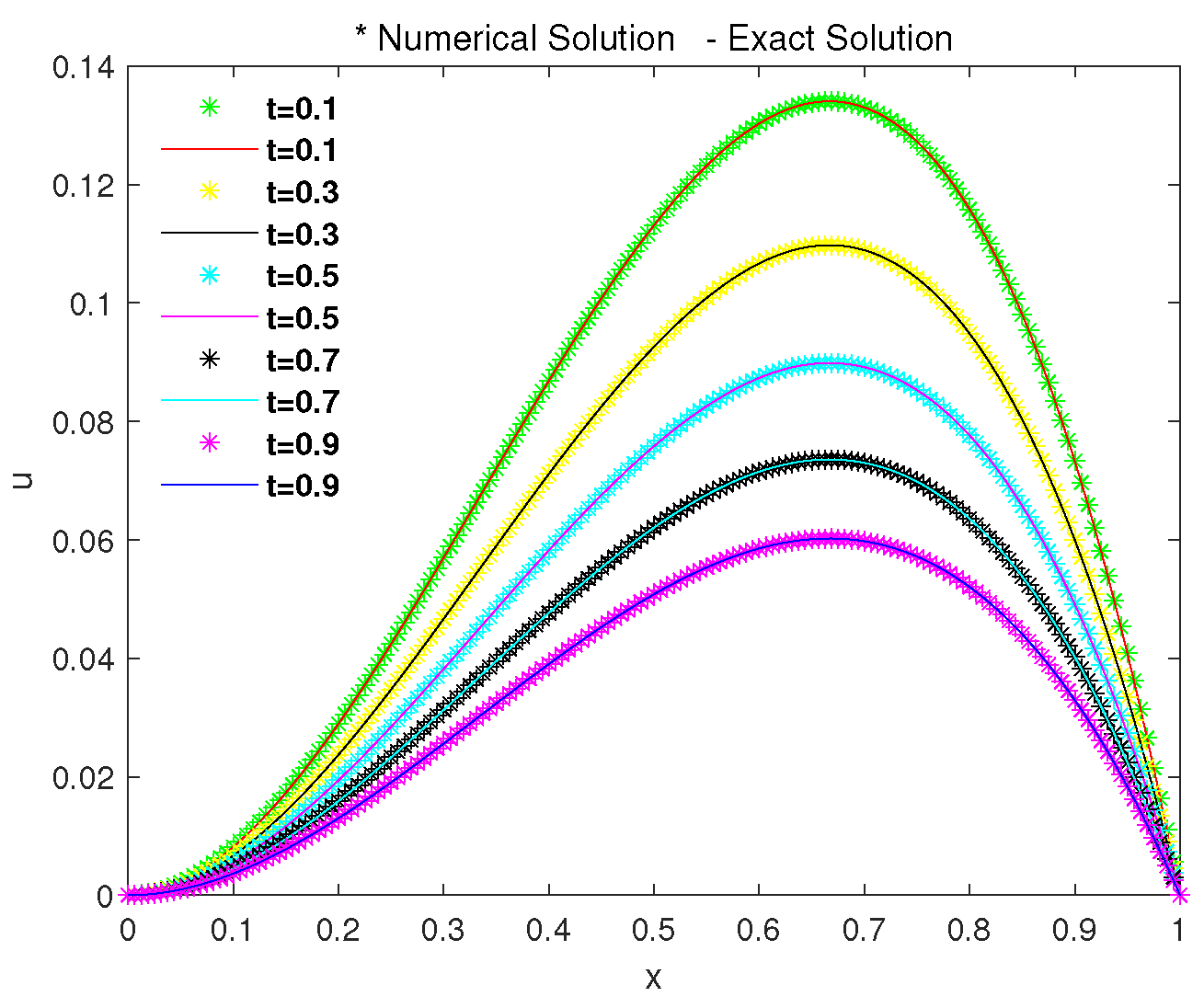
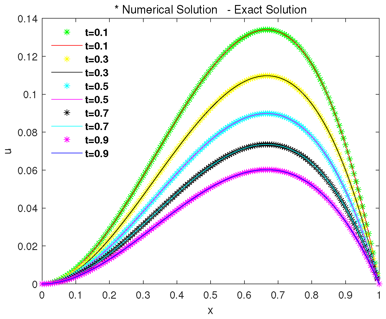
Setting the space step size to , the time step size to , and , Figure 1 shows the comparison between the exact solution (line) and the numerical solution (star) of the weighted explicit finite difference method at (where to with an interval of ). Figure 2 shows a comparison between the analytical solution (line) and the numerical solution (star) of the reduced-dimension weighted explicit finite difference method for Equation (45). In Figure 1 and Figure 2, it can be observed that the numerical solution of Equation (45) is in good agreement with the analytical solution, which further demonstrates the effectiveness of the method.
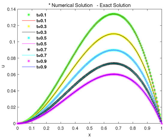
Figure 1.
The numerical and analytical solution comparison for the weighted explicit finite difference method.
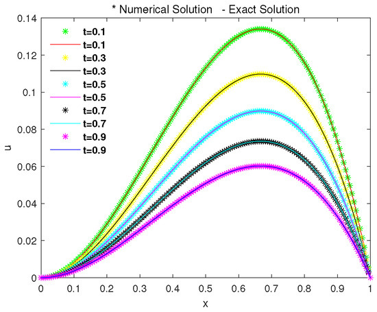
Figure 2.
The numerical and analytical solution comparison for the reduced-dimension weighted explicit finite difference method.
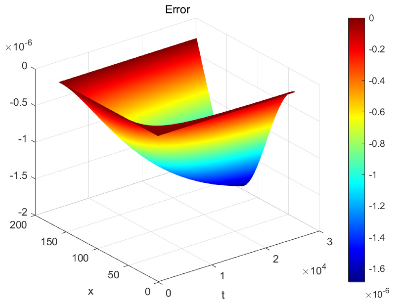
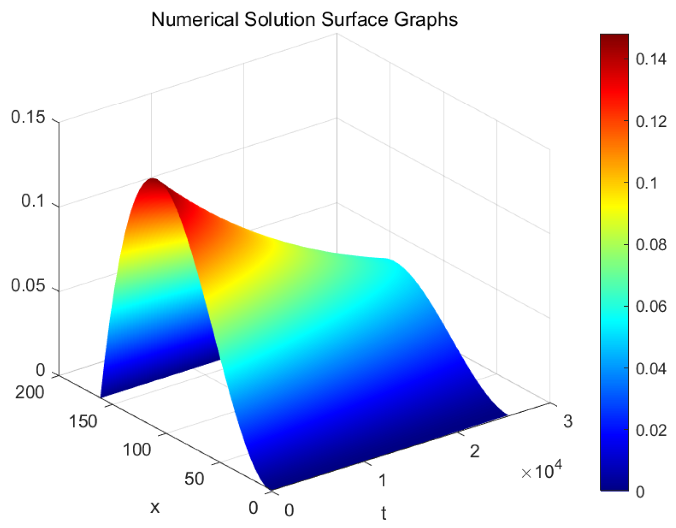
Figure 3 and Figure 4 present the three-dimensional error figures for the two schemes. Figure 5 and Figure 6, respectively, illustrate surface graphs representing the relationship between the numerical solution and the space–time axis for the two methods. Furthermore, Figure 3 and Figure 4 demonstrate that the error between the exact solution and the numerical solutions for both the POD reduced-dimension weighted explicit finite difference method and the weighted explicit finite difference method can reach when the space step size is , the time step size is , and . This observation is consistent with the numerical results presented in Table 1.

Figure 3.
The error figure for the weighted explicit finite difference method.
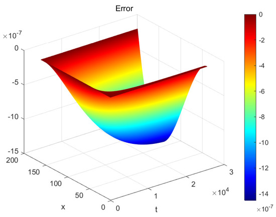
Figure 4.
The error figure for the reduced-dimension weighted explicit finite difference method.

Figure 5.
The surface figure for the weighted explicit finite difference method.

Figure 6.
The surface figure for the reduced-dimension weighted explicit finite difference method.

Table 1.
Comparison of POD method and finite difference method when .
To verify that the reduced-dimension weighted explicit finite difference method ensures sufficient accuracy, reduces degrees of freedom, saves CPU computation time, and improves computational efficiency, we next analyze the error, convergence order, and CPU running time of Equation (45) at , , and .
Since the error order is , the relationship is exploited in the calculation to compensate for the errors caused by the discrete time and space directions. For this purpose, the time step size is set to , and the space grid parameter h takes the values , , and . Table 1 gives the errors, convergence orders, and CPU running time (in seconds) of and in the norm for the weighted explicit finite difference approach and the reduced-dimension weighted explicit finite difference method, with a final time of and a parameter value of . The convergence rates of and , as shown in Table 1, are nearly at the second order under the norm. Notably, the reduced-dimension weighted explicit finite difference method, which uses only six degrees of freedom at each time node, demonstrates a significant advantage in terms of computational efficiency. Furthermore, Table 1 also shows that the CPU running time for the weighted explicit finite difference method is 10 times that of the POD reduced-dimension weighted explicit finite difference method.
Building on the findings in Table 1, Table 2 and Table 3 extend the analysis to different final times, and , respectively. They provide a detailed comparison of the errors, convergence rates, and CPU running times for both the weighted explicit finite difference method and the reduced-dimension weighted explicit finite difference method. Importantly, Table 3 indicates that the CPU running time for the weighted explicit finite difference method ranges from 10 to 17 times that of the POD reduced-dimension method. Furthermore, when the space step size is , the numerical errors are consistent with theoretical calculations, both attaining an accuracy of . Nearly second-order convergence rates can also be observed in Table 3. These tables provide a comprehensive comparison of the errors, convergence rates, and CPU running times for both the weighted explicit finite difference method and the reduced-dimension variant. The results further substantiate the efficiency and accuracy of the reduced-dimension method.
Table 2.
Comparison of POD method and finite difference method when .
Table 3.
Comparison of POD method and finite difference method when .
Continuing the analysis, when the space step size h decreases, the convergence rate of errors and , as indicated in Table 4, approaches the second order for an value of or and a T of 1, 2, or 3. Moreover, the CPU running time for the reduced-dimension weighted explicit finite difference method is observed to be faster than that for the traditional weighted explicit finite difference approach.
Table 4.
Comparison of POD method and finite difference method.
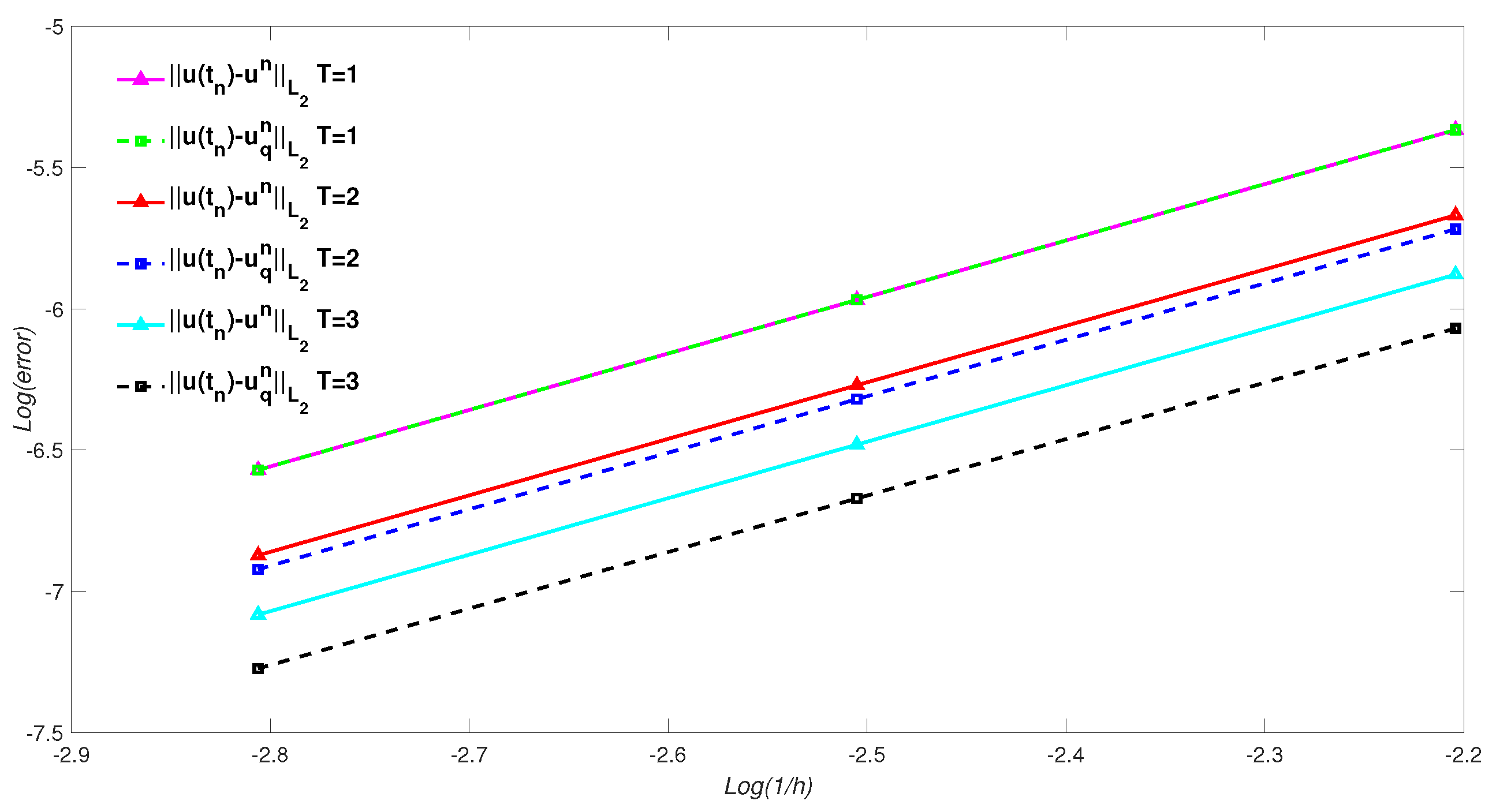
Therefore, based on the data presented in Table 1, Table 2, Table 3 and Table 4, the numerical errors are in line with theoretical expectations, regardless of the specific value chosen for within the tested range (). Moreover, these results highlight the proposed scheme’s capability to ensure sufficient accuracy while reducing degrees of freedom, saving CPU computation time, and enhancing computational efficiency. Additionally, Figure 7 visually presents a comparison of the errors between the two methods when , further illustrating the validity of the reduced-dimension method.
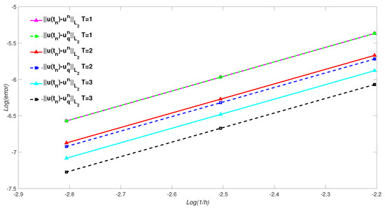
Figure 7.
A comparison of the errors for and at .
Example 2.
Consider the following initial boundary value problems:
in which the diffusion coefficient is and the exact solution is the same as in Example 1.
According to Formula (44), the following source term can be obtained:
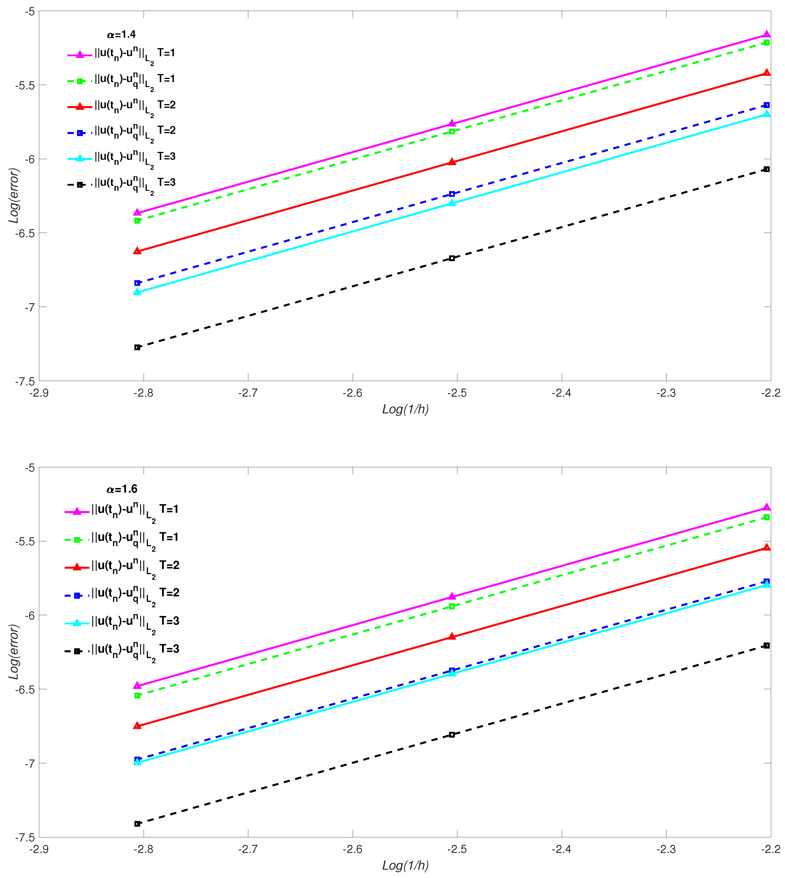
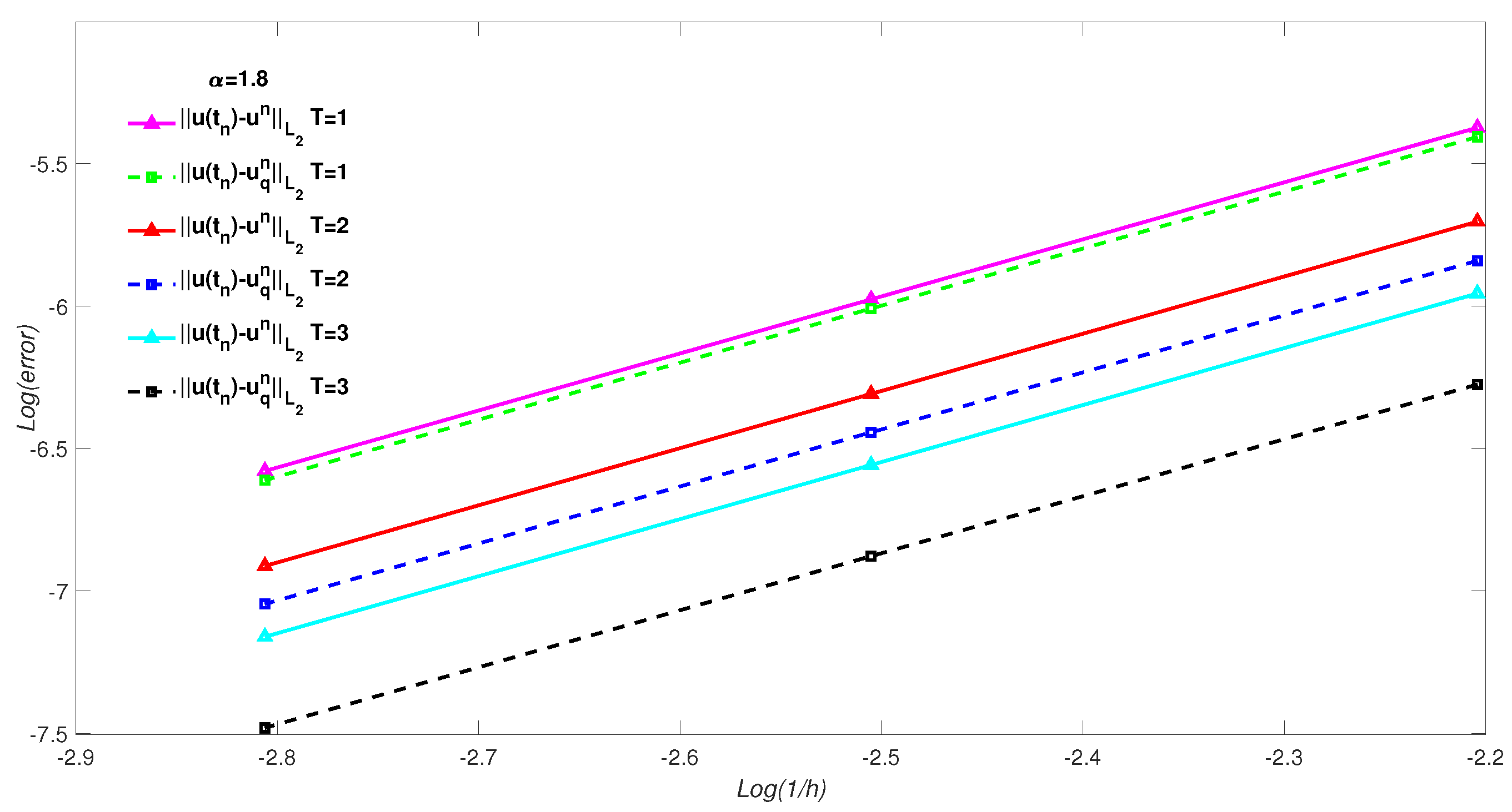
In Table 5, with a time step of and various space meshes of , , and , the orders of convergence for and are observed to be close to 2. The observed convergence is in line with theoretical projections. Additionally, we present the CPU running time results for both methods, corresponding to different values of , , and and for the final time T of 1, 2, and 3. The numerical results for the CPU running time confirm the effectiveness of the reduced-dimension weighted explicit finite difference method. Furthermore, Figure 8 provides a more intuitive comparison of the error estimates between the two methods under various conditions. Specifically, it illustrates the error estimates for different values of (1.4, 1.6, and 1.8) and final times T (1, 2, and 3).
Table 5.
Comparison of POD method and finite difference method.
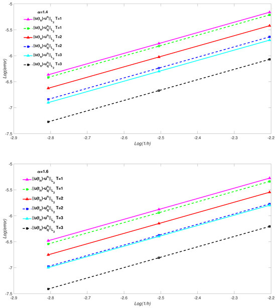
Figure 8.
A comparison of the errors for and at , and .
6. Conclusions
In this paper, we investigate a reduced-dimension weighted explicit finite difference scheme for the space-fractional diffusion equation. The weighted explicit finite difference scheme for the space-fractional diffusion equation is first presented and formulated into a matrix form. In addition, the uniqueness of the weighted explicit finite difference solutions is demonstrated. Subsequently, the POD technique is utilized to establish the matrix form of the reduced-dimension weighted explicit finite difference method, and the implementation steps of the algorithm of the POD reduced-dimension technique are described. We discuss the uniqueness, stability, and error estimation of the solutions.
Numerical simulations were conducted to substantiate the analysis’s correctness and to compare the POD method with the original weighted explicit finite difference scheme. The results indicate that the proposed POD scheme ensures sufficient precision while reducing the degrees of freedom, conserving CPU computation time, and enhancing computational efficiency. Consequently, the reduced-dimension method, leveraging the POD technique, shows promise for broader applications. This approach is potentially applicable to solving other complex partial differential equations in two or higher dimensions.
Author Contributions
Conceptualization, X.R. and H.L.; methodology, X.R.; numerical simulation, X.R.; formal analysis, X.R.; writing—original draft preparation, X.R.; validation, X.R. and H.L.; writing—review, H.L.; supervision, H.L. All authors have read and agreed to the published version of the manuscript.
Funding
This research was funded by the National Natural Science Foundation of China (12161063) and the Programfor Innovative Research Teamin Universities of InnerMongolia Autonomous Region (NMGIRT2207).
Data Availability Statement
No new data were created or analyzed in this study. Data sharing is not applicable to this article.
Acknowledgments
The authors would like to thank the reviewers and editors for their invaluable comments, which greatly refined the content of this article.
Conflicts of Interest
The authors declare no conflicts of interest.
Abbreviations
The following abbreviations are used in this manuscript:
| POD | proper orthogonal decomposition |
References
- Meerschaert, M.M.; Tadjeran, C. Finite difference approximations for fractional advection-dispersion flow equations. J. Comput. Appl. Math. 2004, 172, 65–77. [Google Scholar] [CrossRef]
- Meerschaert, M.M.; Tadjeran, C. Finite difference approximations for two-sided space-fractional partial differential equations. Appl. Numer. Math. 2006, 56, 80–90. [Google Scholar] [CrossRef]
- Podlubny, I. Fractional Differential Equations; Academic Press: New York, NY, USA, 1999. [Google Scholar]
- Bouchaud, J.P.; Georges, A. Anomalous diffusion in disordered media: Statistical mechanisms, models and physical applications. Phys. Rep. 1990, 195, 127–293. [Google Scholar] [CrossRef]
- Raberto, M.; Scalas, E.; Mainardi, F. Waiting-times and returns in high-frequency financial data: An empirical study. Physica A 2002, 314, 749–755. [Google Scholar] [CrossRef]
- Baeumer, B.; Benson, D.A.; Meerschaert, M.M.; Wheatcraft, S.W. Subordinated advection-dispersion equation for Contaminant transport. Water Resour. Res. 2001, 37, 1543–1550. [Google Scholar] [CrossRef]
- Benson, D.A.; Meerschaert, M.M.; Wheatcraft, S.W. The fractional-order governing equation of Lévy motion. Water Resour. Res. 2000, 36, 1413–1424. [Google Scholar] [CrossRef]
- Chechkin, A.V.; Gorenflo, R.; Sokolov, I.M. Retarding subdiffusion and accelerating superdiffusion governed by distributed-order fractional diffusion equations. Phys. Rev. E Stat. Nonlinear Soft Matter Phys. 2002, 66, 046129. [Google Scholar] [CrossRef] [PubMed]
- Krepysheva, N.; Pietro, D.L.; Néel, M.-C. Space-fractional advection-diffusion and reflective boundary condition. Phys. Rev. E Stat. Nonlinear Soft Matter Phys. 2006, 73, 021104. [Google Scholar] [CrossRef] [PubMed]
- Negrete, D.C.; Carreras, B.A.; Lynch, V.E. Front dynamics in reaction-diffusion systems with levy flights: A fractional diffusion approach. Phys. Rev. Lett. 2003, 91, 018302. [Google Scholar] [CrossRef]
- Celik, C.; Duman, M. Crank-Nicolson method for the fractional diffusion equation with the Riesz fractional derivative. J. Comput. Phys. 2012, 231, 1743–1750. [Google Scholar] [CrossRef]
- Yang, Q.; Liu, F.; Turner, I. Numerical methods for fractional partial differential equations with Riesz space fractional derivatives. Appl. Math. Model 2010, 34, 200–218. [Google Scholar] [CrossRef]
- Wang, X.Y.; Zhu, L.; Rui, H.X. A weighted explicit finite difference method for space fractional diffusion equation. J. Ningxia Univ. 2014, 35, 1–5. (In Chinese) [Google Scholar]
- Savović, S.; Djordjevich, A.; Tse, P.W.; Nikezi, D. Explicit finite difference solution of the diffusion equation describing the flow of radon through soil. Appl. Radiat. Isotopes 2011, 69, 237–240. [Google Scholar] [CrossRef]
- Savović, S.; Ivanović, M.; Min, R. A Comparative Study of the Explicit Finite Difference Method and Physics-Informed Neural Networks for Solving the Burgers’ Equation. Axioms 2023, 12, 982. [Google Scholar] [CrossRef]
- Holmes, P.; Lumley, J.L.; Berkooz, G.; Rowley, C.W. Turbulence, Coherent Structures, Dynamical Systems and Symmetry; Cambridge University Press: New York, NY, USA, 2012. [Google Scholar]
- Luo, Z.D.; Chen, G. Proper Orthogonal Decomposition Methods for Partial Differential Equations; Academic Press of Elsevier: San Diego, CA, USA, 2018. [Google Scholar]
- Volkwein, S. Proper Orthogonal Decomposition: Applications in Optimization and Control. 2007. Available online: http://www.math.uni-konstanz.de/numerik/personen/volkwein/teaching/Lecture-Notes-Volkwein.pdf (accessed on 27 May 2024).
- Sirovich, L. Turbulence and the dynamics of coherent structures. Part I: Coherent structures. Q. Appl. Math. 1987, 45, 561–571. [Google Scholar] [CrossRef]
- Sirovich, L. Turbulence and the dynamics of coherent structures. Part II: Symmetries and transformations. Q. Appl. Math. 1987, 45, 573–582. [Google Scholar] [CrossRef]
- Sirovich, L. Turbulence and the dynamics of coherent structures. Part III: Dynamics and scaling, quarterly of applied mathematics. Q. Appl. Math. 1987, 45, 583–590. [Google Scholar] [CrossRef]
- Jolliffe, I.T. Principal Component Analysis; Springer: New York, NY, USA, 1986. [Google Scholar]
- Fukunaga, F. Introduction to Statistical Recognition; Academic Press: New York, NY, USA, 1990. [Google Scholar]
- Selten, F.M. Baroclinic empirical orthogonal functions as basis functions in an atmospheric model. J. Atmos. Sci. 1997, 54, 2099–2114. [Google Scholar] [CrossRef]
- Crommelin, D.T.; Majda, A.J. Strategies for Model Reduction: Comparing Different Optimal Bases. J. Atmos. Sci. 2004, 61, 2206–2217. [Google Scholar] [CrossRef]
- Li, H.; Luo, Z.D.; Gao, J.Q. A new reduced-order FVE algorithm based on POD method for viscoelastic equations. Acta Math. Sci. 2013, 33, 1076–1098. [Google Scholar] [CrossRef]
- Luo, Z.D.; Du, J.; Xie, Z.H.; Guo, Y. A reduced stabilized mixed finite element formulation based on proper orthogonal decomposition for the non-stationary Navier-Stokes equations. Int. J. Numer. Meth. Eng. 2011, 88, 31–46. [Google Scholar] [CrossRef]
- Li, Y.J.; Luo, Z.D.; Liu, C.A. The mixed finite element reduced-dimension technique with unchanged basis functions for hydrodynamic equation. Mathematics 2023, 11, 807. [Google Scholar] [CrossRef]
- Luo, Z.D.; Yang, J. The reduced-order method of continuous space-time finite element scheme for the non-stationary incompressible flows. J. Comput. Phys. 2022, 456, 111044. [Google Scholar] [CrossRef]
- Yang, J.; Luo, Z.D. A reduced-order extrapolating space-time continuous finite element method for the 2D Sobolev equation. Numer. Methods Partial Differ. Equ. 2020, 36, 1446–1459. [Google Scholar] [CrossRef]
- Luo, Z.D.; Jin, S.J. A reduced-order extrapolated Crank-Nicolson collocation spectral method based on proper orthogonal decomposition for the two-dimensional viscoelastic wave equations. Numer. Methods Partial Differ. Equ. 2020, 36, 49–65. [Google Scholar] [CrossRef]
- Luo, Z.D.; Jiang, W. A reduced-order extrapolated Crank-Nicolson finite spectral element method for the 2D non-stationary Navier-Stokes equations about vorticity-stream functions. Appl. Numer. Math. 2020, 147, 161–173. [Google Scholar] [CrossRef]
- Luo, Z.D.; Li, H.; Sun, P.; Gao, J.Q. A reduced-order finite difference extrapolation algorithm based on POD technique for the non-stationary Navier-Stokes equations. Appl. Math. Model 2013, 37, 5464–5473. [Google Scholar] [CrossRef]
- An, J.; Luo, Z.D.; Li, H.; Sun, P. A reduced spectral-finite difference scheme based on POD method and posterior error estimate for the three-dimensional parabolic equation. Front. Math. China 2015, 10, 1025–1040. [Google Scholar] [CrossRef]
- Luo, Z.D.; Ren, H.L. A reduced-order extrapolated finite difference iterative method for the Riemann-Liouville tempered fractional derivative equation. Appl. Numer. Math. 2020, 157, 307–314. [Google Scholar] [CrossRef]
- Deng, Q.X.; Luo, Z.D. A reduced-order extrapolated finite difference iterative scheme for uniform transmission line equation. Appl. Numer. Math. 2022, 172, 514–524. [Google Scholar] [CrossRef]
- Sun, Z.Z.; Gao, G.H. Finite-Difference Method for Fractional Differential Equations; Chinese Science Press: Beijing, China, 2015. (In Chinese) [Google Scholar]
- Zhang, W.S. Finite Difference Methods for Partial Differential Equations in Science Computation; Higher Education Press: Beijing, China, 2006. (In Chinese) [Google Scholar]
- Quarteroni, A.; Sacco, R.; Saleri, F. Numerical Mathematics; Springer: New York, NY, USA, 2000. [Google Scholar]


Disclaimer/Publisher’s Note: The statements, opinions and data contained in all publications are solely those of the individual author(s) and contributor(s) and not of MDPI and/or the editor(s). MDPI and/or the editor(s) disclaim responsibility for any injury to people or property resulting from any ideas, methods, instructions or products referred to in the content. |
© 2024 by the authors. Licensee MDPI, Basel, Switzerland. This article is an open access article distributed under the terms and conditions of the Creative Commons Attribution (CC BY) license (https://creativecommons.org/licenses/by/4.0/).