Abstract
In the presence of Banach spaces, a novel iterative algorithm is presented in this study using the Chatterjea–Suzuki–C (CSC) condition, and the convergence theorems are established. The efficacy of the proposed algorithm is discussed analytically and numerically. We explain the solution of the Caputo fractional differential problem using our main result and then provide the numerical simulation to validate the results. Moreover, we use MATLAB R (2021a) to compare the obtained numerical results using the new iterative algorithm with some efficient existing algorithms. The work seems to contribute to the current advancement of fixed-point approximation iterative techniques in Banach spaces.
Keywords:
strong convergence; Chatterjea–Suzuki–C condition; fixed point; iterative algorithm; fractional differential equation MSC:
47H10; 47J25
1. Introduction and Motivation
To approximate the value of a fixed point (a point that does not change under certain conditions), various iterative algorithms have been introduced over time in the field of fixed-point theory [1]. Fixed-point theory is a fundamental concept in mathematics with significant applications. For example, by identifying fixed points [2], researchers can gain insights into the behavior of iterative algorithms, which are commonly used in logic programming [3], machine learning [4], and other artificial intelligence applications [5]. This provides a framework for understanding the convergence of these algorithms and making predictions about their performance. Moreover, fixed-point theory is a crucial tool for the geometry of figures [6,7,8] that is important in improving the performance of modern systems and advancing the field of artificial intelligence by developing and improving fractal antennas. The speed of convergence is an important factor when choosing between different iterative algorithms for approximating fixed points. Once the existence of a fixed point for a given mapping has been established, determining its value becomes a challenging task. Therefore, some basic iterative algorithms are discussed in [9,10,11], and further modifications concerning these fundamental algorithms have been developed in [12,13,14]. By studying the literature [9,10,11,12,13,14], it can be observed that every modified iterative algorithm has an improved degree of convergence compared to the previous one, and authors proved their claims with the help of numerical examples. Furthermore, the Banach contraction principle [15] provides a powerful tool for establishing the existence and uniqueness of a fixed point, but it does not provide any direct method for computing a fixed point itself. The Banach contraction theorem refers simply to Picard’s iterative scheme [10] to find the approximation for the value of a fixed point. Therefore, the role of iterative methods becomes more significant for this purpose. A related review of the literature demonstrates that the novel and generalized classes of Kannan-type contractions are used to discuss new results in [16,17,18]. Generalized nonexpansive mappings on Banach space are also discussed in [19,20,21,22]. Moreover, significant results are available in the literature after extensive study of mappings with the Suzuki (C)-condition. Khatoon and Uddin [23], Wairojjana [24], and Hasanen [25,26,27] also presented iterative algorithms in this respect. More recently, solutions to non-linear problems have been found using iterative schemes. For instance, an innovative iterative method was presented for determining an approximate solution of a certain kind of fractional differential equation in [28].
Ullah and Arshad [22] presented the M-Iterative algorithm along with condition (C). Furthermore, [22] contains a beautiful discussion about why each new iteration process is preferred over a large class of the existing iterative algorithms. More recently, [29] used the M-Iterative algorithm defined in [22] along with the Chatterjea–Suzuki–C condition and established new results related to strong and weak convergence. Hence, according to the above review of the literature, the following question arises, which is posed and answered in this research.
Question: Is there any iterative scheme with a better rate of convergence compared to the algorithm discussed in [29]?
To answer this question, we introduce a new three-step iterative algorithm, the Z-Iterative algorithm, in this research. To present the efficiency of our proposed algorithm, we plan this article as follows:
In Section 2, we go over the prerequisites and necessary terminology pertaining to various iterations. Then, in Section 3, we demonstrated strong and weak convergence results using the Z-iterative approach in the context of uniformly convex Banach spaces. Using nonexpansive mapping enhanced with the Chatterjea–Suzuki–C condition, this criterion is demonstrated. Theorems are another way in which these conditions are further refined and proven. Section 4 offers an application to fractional differential equations. In light of this, the suggested iteration technique’s Section 5 presents a range of numerical outcomes by considering various parameter values. This section also compares these numerical values using a class of existing iterations and the new proposed iteration. Tabular and graphical illustrations are used to conduct time analysis for the number of iterations. To demonstrate that the examined scheme is superior to the current ones, we also make a numerical comparison of the Z-iterative algorithm’s convergence speed with some other well-known schemes. Section 6 concludes and provides more discussion of these findings and comparisons. Future directions for this work are also included in the last Section.
2. Preliminaries
Fundamental definitions and theorems that are necessary to demonstrate our new findings are provided in this section. In the subsequent definitions, ℵ denotes a nonempty subset of uniformly convex Banach space ℜ.
Definition 1
([30,31]). A mapping is said to be a contraction if for all elements there exists α in such that
Definition 2.
τ is a nonexpansive mapping over the uniformly convex Banach space ℜ if
Definition 3.
A point is a fixed point of mapping τ if
We denote the set of such fixed points of τ by .
Definition 4.
A mapping is said to be endowed with a condition (C) (or Suzuki mapping) if the following inequality holds
Definition 5.
A mapping is said to satisfy Chatterjea–Suzuki–C condition if it satisfies the following inclusion:
Definition 6
([32]). A mapping τ defined on a subset ℵ of a Banach space is a contraction on the uniformly convex Banach space if and only if there is a function
such that
where and e ∈ℵ, is the distance between o and .
Definition 7.
Suppose ℵ is a closed and convex subset of ℜ. If is a bounded set, then the following mapping is called the asymptotic radius of corresponding to ℵ,
Similarly, asymptotic center of sequence corresponding to ℵ is defined by
Definition 8
([33]). Opial’s condition holds in a Banach space ℜ if and only if a sequence in ℜ converges in the weak sense to and
Remark 1
([34]). If ℜ is a uniformly convex Banach space, then the set contains one element. Moreover, if ℵ is weakly convex and compact then is a convex set. More details can be seen in [35,36].
Proposition 1.
For a nonempty closed subset ℵ of a Banach space, we have the following results in the presence of self-mapping
- (a)
- If τ is enhanced with Chatterjea–Suzuki–C condition and then
- (b)
- If τ is enhanced with the condition of Chatterjea–Suzuki–C, then is closed. Moreover, if ℜ is strictly convex and ℵ is convex, then is also convex.
- (c)
- If τ is enhanced with the condition namely Chatterjea–Suzuki–C, then for any .
- (d)
- If τ is enhanced with Chatterjea–Suzuki–C condition, is weakly convergent to a, andthen provided that ℜ satisfies Opial’s condition.
The subsequent result is initiated by [37].
Lemma 1.
For a real number , consider and in ℜ satisfying
and
then
Iterative Algorithms
The most simple and basic among the existing iterative algorithms is the Picard [10] iterative algorithm defined by , which is commonly used to find approximations. In the following paragraph, we enlist some more advanced and recent iterative algorithms that are used and compared with our new iteration in this study. Moreover, and denote sequences in for the following iteration schemes.
Agarwal et al. [12] defined the iterative algorithm as given by,
Abbas and Nazir [13] defined the iterative algorithm as given by,
Thakur et al. [14] defined the iterative algorithm as given by,
M-iterative algorithm is defined in [22] (see, also [29])
3. Main Results
In this section, we propose our new iterative algorithm and name it the Z-iterative algorithm, defined as follows
where , are sequences in (0, 1). The main results are obtained using (9), which demonstrates the efficiency of our proposed algorithm.
Lemma 2.
Let ℜ be a uniformly convex Banach space and ℵ be a nonempty closed convex subset of ℜ. Suppose is enhanced with the condition of Chatterjea–Suzuki–C along with . Moreover, if the sequence is as defined in Equation (9) then holds true for each .
Proof.
Let be an arbitrary element in then because of Proposition 1 (a), we obtain
Next, using the algorithm (9), we have
Then, making use of (10), we obtain
Now, using Chatterjea–Suzuki–C condition with we have
Using the above inequality in (11), we obtain
Next, we have
By using Chatterjea–Suzuki–C condition with , we obtain
Next, by combining it with (13), we obtain
Hence, we obtain
and using (14), we can write
Continuing in this way, from (12), (14), and (16), we conclude that
which implies that
This shows that is decreasing and bounded for each . Hence,
exists. □
Theorem 1.
Let and be the same as in Lemma 2, then if and only if the sequence is bounded and .
Proof.
Consider then from Lemma 2, we infer that exists and is bounded. Assume that
and we want to show that
Therefore, from (12), we have
which implies that
and combining it with (17), we obtain
Since , therefore using Proposition 1 (a), we obtain
which implies that
Then, using (16), we have
and combining it with (17), we obtain
Next, using (18) and (20), we obtain
Moreover,
Hence,
Then using (17), (19), and (21) along with Lemma 1, we obtain
Conversely, let is bounded with
here we will show that Let , then using definition (7)
and using Proposition 1 (c), we obtain
Hence, . Since contains singleton point, so , i.e., and □
Theorem 2.
Suppose and are the same as in Lemma 2 and ℵ is a weakly compact and convex subset of ℜ then has week convergence to a point in in the presence of ℜ with the condition of Opial.
Proof.
Lemma 2, implies that exists and we want to show that has a unique weak subsequential limit in . Since ℵ is weakly compact, let and be the subsequential limits of subsequences and of , respectively. By Theorem 1, we have
and
At this step, we aim to show the uniqueness. Therefore, if then by Opial’s condition, we have
which shows that
This is not possible and leads to a contradiction. Hence, converges weakly to a point in . □
Theorem 3.
Suppose and are the same as in Lemma 2 as well as ℵ is a weakly compact and convex subset of ℜ then converges strongly to a point in .
Proof.
By Theorem (1), we have
and since ℵ is compact and , so has a subsequence for some such that
Furthermore, because of Proposition 1 (c), we have
which shows that as . This implies that i-e and exists by Lemma 2. Hence converges strongly to . □
Lemma 3.
The sequence has strong convergence to a point in with where and are assumed to have the same properties as in Lemma 2.
Proof.
For all , Lemma (2) suggests the existence of
and by assumption, it follows that
According to Proposition 1 (b), the set is indeed closed in ℵ and then the remaining proof closely follows from the proof of ([36], Theorem 2) and can be omitted. □
This leads us to suggest another strong convergence theorem that does not require assuming the compactness of the domain. This is an exciting advancement that expands the applicability of the theorem.
Theorem 4.
Let and be the same as in Lemma 2, then converges strongly to a point in whenever τ is a contraction on the uniformly convex Banach space.
Proof.
From Theorem 1, we have
which implies that
□
The successful proof of all the assumptions in Theorem 4 confirms that the sequence essentially converges strongly in . This is a significant result that demonstrates the reliability and effectiveness of the method.
4. Application to Caputo Fractional Differential Equation
This century has dealt with the extensive study of fractional differential equations (FDEs) due to their interesting and important applications in different areas of science. For example, fractional differential equations have been used in the modeling of complex phenomena, such as fractals, anomalous diffusion, and non-local interactions. Its applications have also been found in finance, biology, image processing, etc. Overall, fractional differential equations have proven to be a powerful tool in the modeling and analysis of complex systems in various fields.
Different types of fractional derivatives are used in the literature according to the model of the problem. We use Caputo-type fractional derivatives generally defined by
where , is a real valued function, is the order of Caputo-type fractional derivative, r is an integer, and New fixed-point results are obtained using non-linear operators in [38], and functional-integral equations are solved in [39,40]. Hence, many problems are challenging to solve using analytical techniques. However, it is still possible to solve them by finding an approximation value through alternative methods. Some researchers have used fixed-point techniques for nonexpansive operators to solve fractional differential equations. For example, see [41].
Let represent the Caputo fractional derivative of order endowed with then we apply the Z-iterative algorithm (9) under the Chatterjea–Suzuki–C for the following fractional differential equation
Let ℑ be a collection of continuous functions that map the interval to . The usual maximum norm is used to determine the size of the functions in ℑ. The respective Green’s function associated with the fractional differential Equation (22) is defined by
Now we proceed to formulate and prove the following theorem.
Theorem 5.
Consider an operator defined by
If the following inclusion holds
then Z-iterative algorithm (9) approaches some solutions S of the fractional differential Equation (22) in case .
Proof.
Since an element f of ℑ is the solution of the fractional differential Equation (22) if and only if it is also the solution to the subsequent equation [29],
Now, for any and , it follows that
Consequently, we obtain
Thus, meets the Chatterjea–Suzuki–C requirement. Based on Lemma 3, the sequence produced by (9) approaches a stationary point of the mapping . This point is the solution to the given fractional differential equation. □
5. Numerical Simulation
In this section, we analyze that the convergence speed of the Z-iterative algorithm is better than the modern algorithms discussed in [12,13,14,29] with the help of a numerical example.
Example 1.
Let be endowed with usual norm and let be a function defined by
we will show that the following conditions hold:
- .
- τ does not satisfy condition (C).
- τ satisfies condition Chatterjea–Suzuki–C.
Proof.
We discuss the above conditions one by one as follows:
- Since implies that τ possesses a single fixed point, and .
- If we take and then τ does not satisfies condition (C).
- To prove the Chatterjea–Suzuki–C condition, we have 4 cases:
- (Case-1) If then, . Hence,
- (Case-2) If then, .
Hence,
- (Case-3) If then, .
Hence,
- (Case-4) If then, .
Hence,
Hence, from the above cases (1–4), part (3) of Example 1 is proved. □
We choose , , and with initial point (7.5) and generate the following Table 1 of the values by performing 30 iterations. We analyze that Agarwal et al. iterative algorithm [35] converges at the 29th iteration while Abbas and Nazir [13] and M [22] iterative algorithms need 19 and 18 iterations, respectively. It is significant to remark that our proposed new algorithm converges to the solution at the 11th iteration, which is a noticeable improvement. However, the M-Iterative algorithm has already been proven efficient over the others [22,29]. The main purpose is now to compare the Z-iterative algorithm and the M-Iterative algorithm. We continue in this way by changing the choice of sequences and initial guesses to obtain numerical values in Table 2 and Table 3. Figure 1 and Figure 2 validate our results.

Table 1.
Numeric outcomes of different iterative algorithms with an initial guess (7.5).
Table 2.
, , and .
Table 3.
, , and .
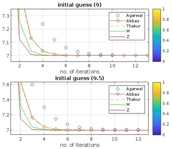
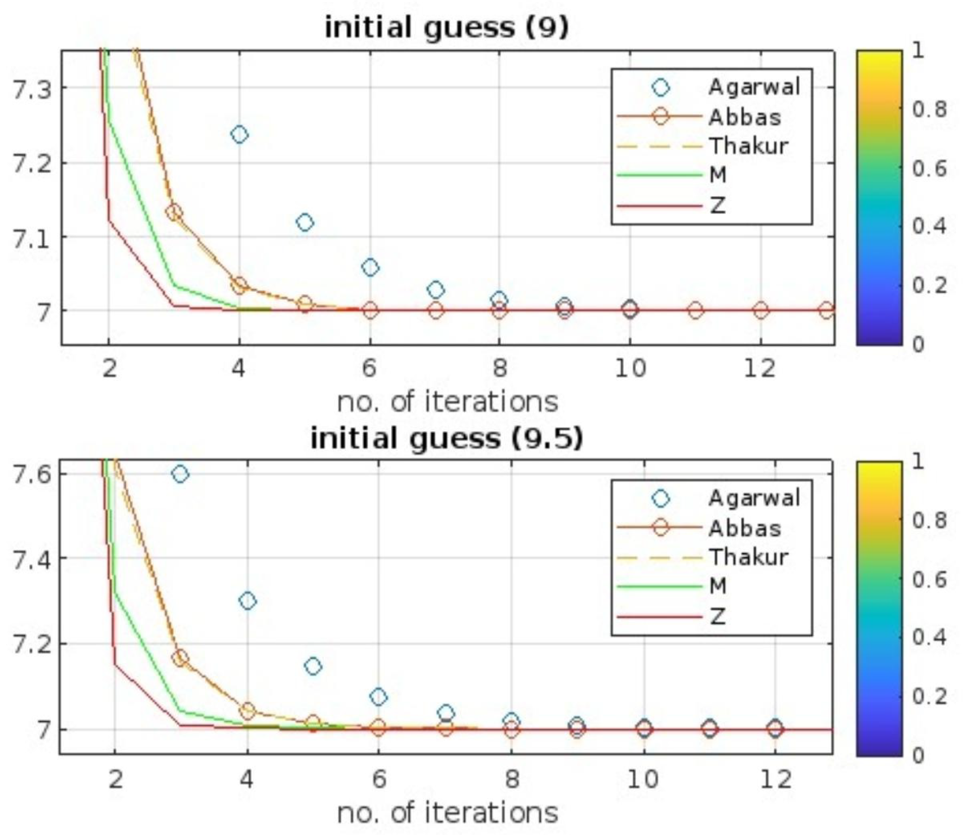
Figure 1.
Comparison of Z-iterative algorithm with other iterative algorithms with initial point (9) and (9.5).

Figure 2.
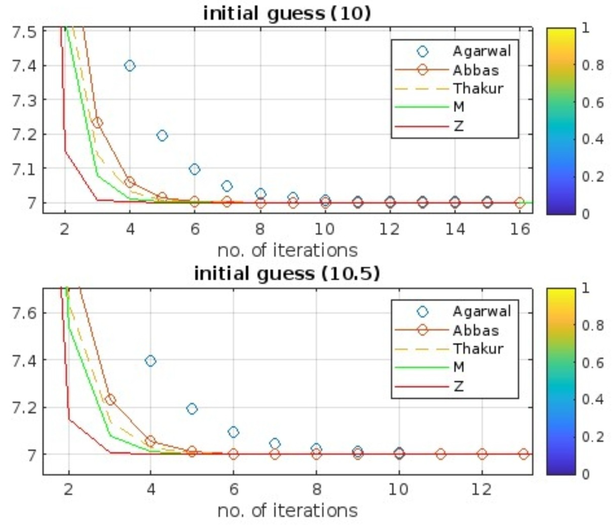
Comparison of Z-iterative algorithm with other iterative algorithms with initial point (10) and (10.5).
By considering the sequences , , and , a significant improvement of the results can be observed between our proposed iterative algorithm and Agarwal et al. iterative algorithm that needs 52 iterations as compared to 13. It is interesting to note that by changing the initial guess from 9 to 9.5, each of the listed algorithms needs one more iteration see Figure 1. Furthermore, by considering the sequences , , and , a significant improvement of the results can be observed between our proposed iterative algorithm and Agarwal et al. iterative algorithm that needs 54 iterations as compared to 11. It is interesting to note that by changing the initial guess from 10 to 10.5, miscellaneous variation in the number of iterations for each of the listed algorithms can be seen in Figure 2.
From the graphical comparison between the Z-iterative algorithm and another existing algorithm, one can observe the fast convergence of the Z-iterative algorithm as demonstrated in Figure 1 and Figure 2, respectively. This faster convergence is a significant advantage of the Z-iterative algorithm, as it allows us to reach the desired solution more quickly and efficiently.
6. Conclusions and Further Discussions
The iterative Z-Algorithm that includes operators enhanced with the Chatterjea–Suzuki–C condition is examined in this study. It shows that, under the right circumstances on the operator or the domain, this technique converges both weakly and strongly to a fixed point of a mapping equipped with the Chatterjea–Suzuki–C condition. Furthermore, we use operators enhanced with the Chatterjea–Suzuki–C condition to solve a fractional differential equation. Furthermore, some tables and graphs are presented to demonstrate the Z-iterative scheme’s higher accuracy in comparison to other existing schemes [12,13,29]. Let us discuss the advantages of our proposed iterative scheme:
- Compared to other schemes in the literature, our approach demonstrates superior convergence to a fixed point. This means that it reaches a stable solution more efficiently and effectively.
- Our proposed iterative scheme stands out by utilizing two scalar sequences , instead of three. This unique approach leads to better convergence in comparison with various other iterative techniques described in the literature.
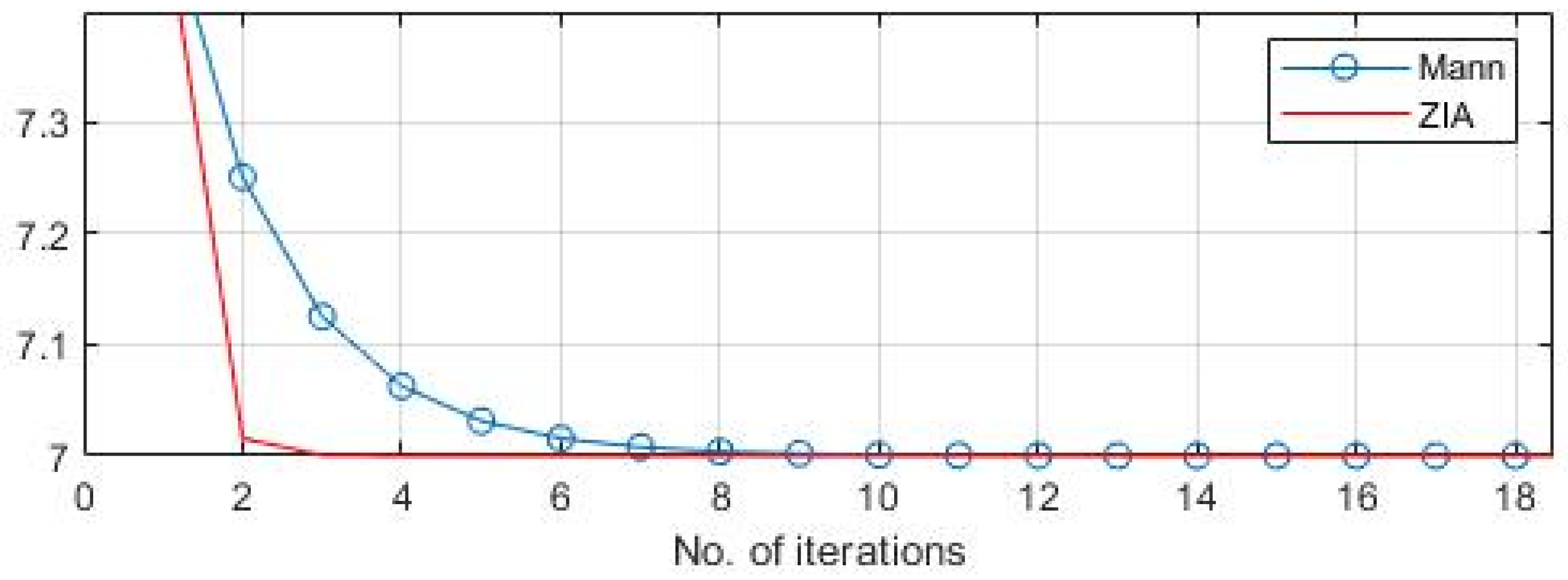
- The proposed iterative scheme has been proven to be stable when it comes to initial points and sequences of scalars. This stability is demonstrated by the data presented in tabular and graphical forms, which clearly shows the consistent and reliable performance of the scheme.In light of the above discussion, we further compared it with the Mann Iterative algorithm ([9]) in Figure 3.
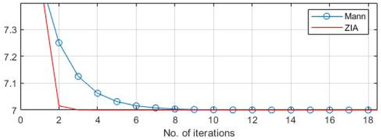 Figure 3. Comparison between Z-iterative algorithm (ZIA) and Mann iterative Algorithm [9].
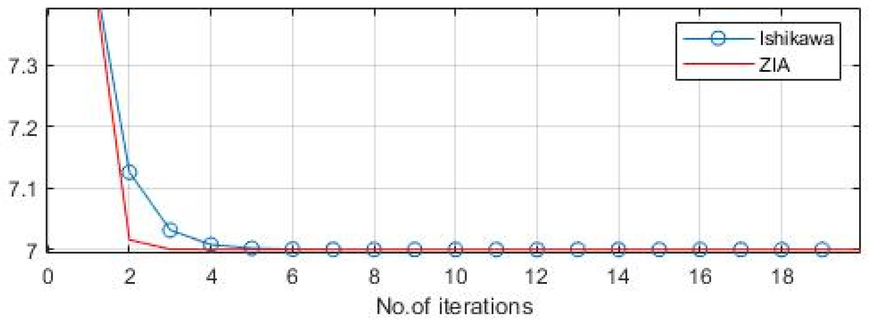
Similarly, we compare with Ishikawa iterative algorithm [11] in Figure 4

Figure 4.
Comparison between Z-iterative algorithm (ZIA) and Ishikawa iterative Algorithm [11].
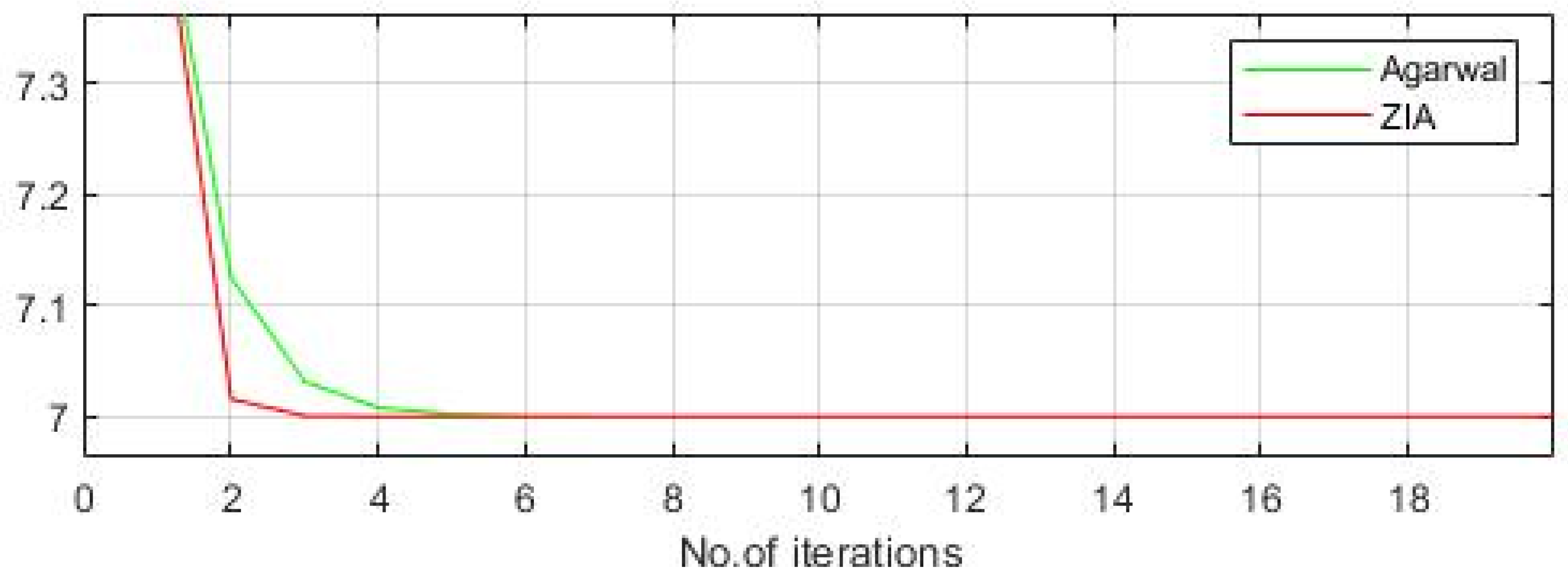
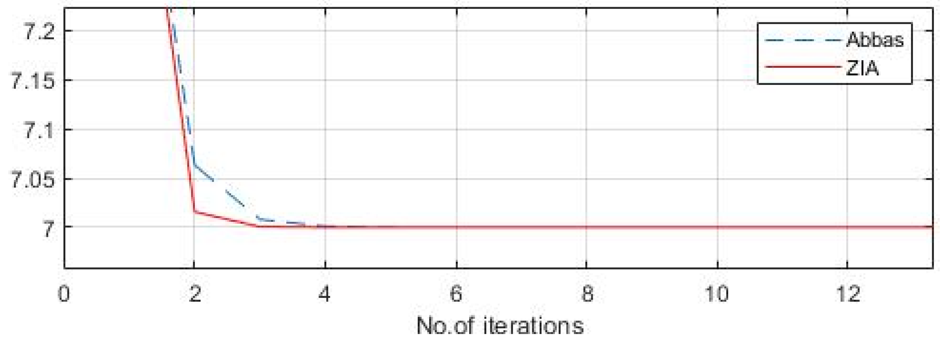
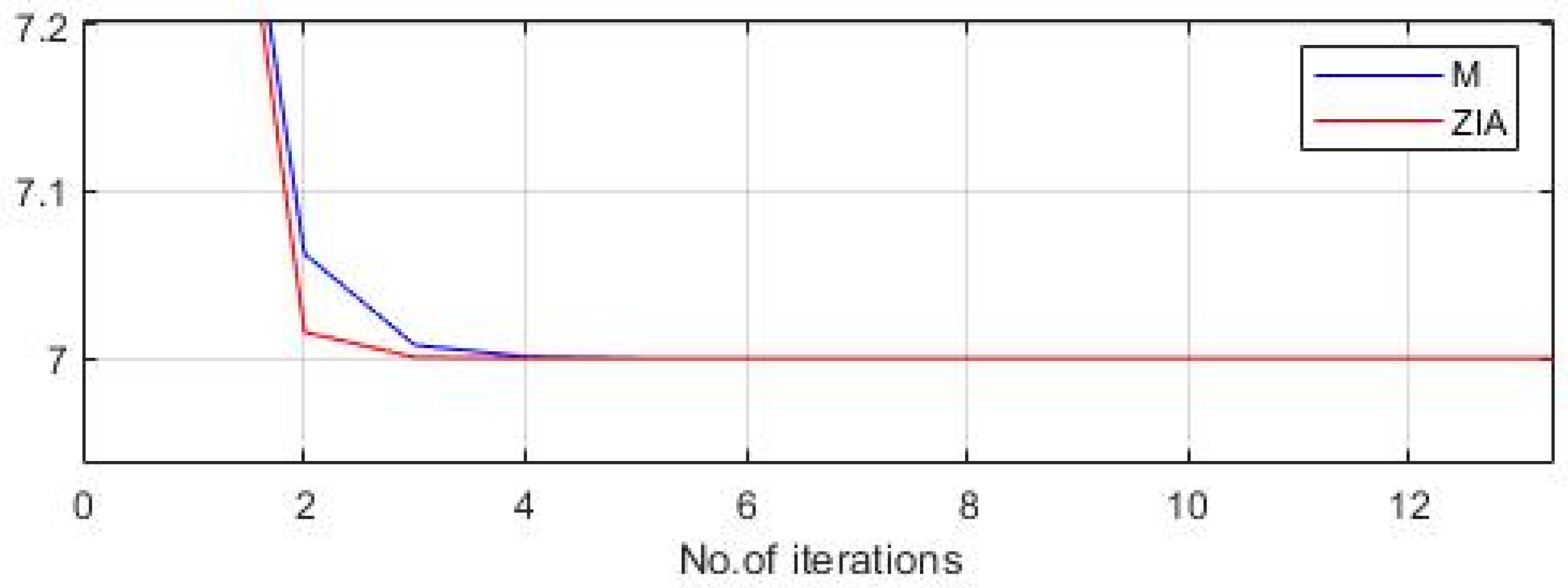
And so forth, the efficiency of our proposed algorithm is vital in comparison to the existing, well-known algorithms (Figure 5, Figure 6 and Figure 7).
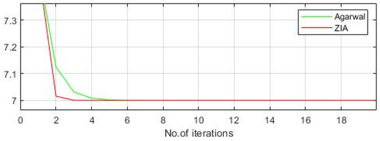
Figure 5.
Further comparison between the Z-iterative algorithm (ZIA) and Agarwal iterative Algorithm.

Figure 6.
Further comparison between the Z-iterative algorithm (ZIA) and Abbas iterative Algorithm.

Figure 7.
Further comparison between the Z-iterative algorithm (ZIA) and M-Iterative Algorithm.
As a result, a decision must be made between various iteration methodologies, with crucial factors taken into account. For example, simplicity and convergence speed are the two most important elements in determining whether the iteration strategy is more effective than others. In cases like this, the following problems will unavoidably arise: Which iteration strategy accelerates convergence among these? This article demonstrates that our proposed iteration scheme converges faster than the present modern iteration schemes. For our future work, we can enhance the results using more generalized (C)-conditions [42]. It may help to improve the convergence rate of our proposed iteration.
Author Contributions
Each author equally contributed to writing and finalizing the article. Conceptualization, R.S. and W.A.; methodology, W.A. and A.T.; software, N.A. validation, N.A. and A.T.; formal analysis, N.A. and A.T.; investigation, R.S. and W.A.; resources, A.T.; writing—original draft preparation, W.A.; writing—review and editing, A.T.; visualization, A.T.; supervision, R.S.; project administration, A.T. and W.A. All authors have read and agreed to the published version of the manuscript.
Funding
This research received no external funding.
Data Availability Statement
No new data were generated for this study.
Acknowledgments
The author extends the appreciation to the Deanship of Postgraduate Studies and Scientific Research at Majmaah University for funding this research work through the project number (PGR-2024-1062).
Conflicts of Interest
The authors declare no conflicts of interest.
References
- Tassaddiq, A.; Ahmed, W.; Zaman, S.; Raza, A.; Islam, U.; Nantomah, K. A Modified Iterative Approach for Fixed Point Problem in Hadamard Spaces. J. Funct. Spaces 2024, 1, 5583824. [Google Scholar] [CrossRef]
- Tassaddiq, A.; Kanwal, S.; Perveen, S.; Srivastava, R. Fixed points of single-valued and multi-valued mappings in sb-metric spaces. J. Inequalities Appl. 2022, 1, 85. [Google Scholar] [CrossRef]
- Khachay, M.Y.; Ogorodnikov, Y.Y. Efficient approximation of the capacitated vehicle routing problem in a metric space of an arbitrary fixed doubling dimension. InDoklady Math. 2020, 102, 324–329. [Google Scholar] [CrossRef]
- Khamsi, M.A.; Misane, D. Fixed point theorems in logic programming. Ann. Math. Artif. Intell. 1997, 21, 231–243. [Google Scholar] [CrossRef]
- Camelo, M.; Papadimitriou, D.; Fàbrega, L.; Vilà, P. Geometric routing with word-metric spaces. IEEE Commun. Lett. 2014, 18, 2125–2128. [Google Scholar] [CrossRef]
- Tassaddiq, A. General escape criteria for the generation of fractals in extended Jungck–Noor orbit. Math. Comput. Simul. 2022, 196, 1–14. [Google Scholar] [CrossRef]
- Tassaddiq, A.; Kalsoom, A.; Rashid, M.; Sehr, K.; Almutairi, D.K. Generating Geometric Patterns Using Complex Polynomials and Iterative Schemes. Axioms 2024, 13, 204. [Google Scholar] [CrossRef]
- Tassaddiq, A.; Tanveer, M.; Azhar, M.; Lakhani, F.; Nazeer, W.; Afzal, Z. Escape criterion for generating fractals using Picard–Thakur hybrid iteration. Alex. Eng. J. 2024, 100, 331–339. [Google Scholar] [CrossRef]
- Mann, W.R. Mean value methods in iteration. Proc. Am. Math. Soc. 1953, 4, 506–510. [Google Scholar] [CrossRef]
- Picard, É. Mémoire sur la théorie des équations aux dérivées partielles et la méthode des approximations successives. J. Mathématiques Pures Appliquées 1890, 6, 145–210. [Google Scholar]
- Ishikawa, S. Fixed points by a new iteration method. Proc. Am. Math. Soc. 1974, 44, 147–150. [Google Scholar] [CrossRef]
- Agarwal, R.P.; O’Regan, D.; Sahu, D.R. Iterative construction of fixed points of nearly asymptotically nonexpansive mappings. J. Nonlinear Convex Anal. 2007, 1, 61. [Google Scholar]
- Abbas, M.; Nazir, T. Some new faster iteration process applied to constrained minimization and feasibility problems. Mat. Vestn. 2014, 66, 223–234. [Google Scholar]
- Thakur, B.S.; Thakur, D.; Postolache, M. A new iterative scheme for numerical reckoning fixed points of Suzuki’s generalized nonexpansive mappings. Appl. Math. Comput. 2016, 275, 147–155. [Google Scholar] [CrossRef]
- Banach, S. Sur les opérations dans les ensembles abstraits et leur application aux équations intégrales. Fundam. Math. 1922, 3, 133–181. [Google Scholar] [CrossRef]
- Konwar, N.; Srivastava, R.; Debnath, P.; Srivastava, H.M. Some new results for a class of multivalued interpolative Kannan-type contractions. Axioms 2022, 11, 76. [Google Scholar] [CrossRef]
- Debnath, P.; Srivastava, H.M. New extensions of Kannan’s and Reich’s fixed point theorems for multivalued maps using Wardowski’s technique with application to integral equations. Symmetry 2020, 12, 1090. [Google Scholar] [CrossRef]
- Debnath, P.; Mitrović, Z.D.; Srivastava, H.M. Fixed points of some asymptotically regular multivalued mappings satisfying a Kannan-type condition. Axioms 2021, 10, 24. [Google Scholar] [CrossRef]
- Suzuki, T. Fixed point theorems and convergence theorems for some generalized nonexpansive mappings. J. Math. Anal. Appl. 2008, 340, 1088–1095. [Google Scholar] [CrossRef]
- Ahmad, J.; Ullah, K.; George, R. Numerical algorithms for solutions of nonlinear problems in some distance spaces. AIMS Math. 2023, 8, 8460–8477. [Google Scholar] [CrossRef]
- Ullah, K.; Ahmad, J.; Mlaiki, N. On Noor iterative process for multi-valued nonexpansive mappings with application. Int. J. Math. Anal. 2019, 13, 293–307. [Google Scholar] [CrossRef]
- Ullah, K.; Arshad, M. Numerical reckoning fixed points for Suzuki’s generalized nonexpansive mappings via new iteration process. Filomat 2018, 32, 187–196. [Google Scholar] [CrossRef]
- Khatoon, S.; Uddin, I. Convergence analysis of modified Abbas iteration process for two G-nonexpansive mappings. Rend. Circ. Mat. Palermo Ser. 2 2021, 70, 31–44. [Google Scholar] [CrossRef]
- Wairojjana, N.; Pakkaranang, N.; Pholasa, N. Strong convergence inertial projection algorithm with self-adaptive step size rule for pseudomonotone variational inequalities in Hilbert spaces. Demonstr. Math. 2021, 54, 110–128. [Google Scholar] [CrossRef]
- Hammad, H.A.; Rehman, H.U.; Zayed, M. Applying faster algorithm for obtaining convergence, stability, and data dependence results with application to functional-integral equations. AIMS Math. 2022, 7, 19026–19056. [Google Scholar] [CrossRef]
- Hammad, H.A.; Rehman, H.U.; De la Sen, M. A novel four-step iterative scheme for approximating the fixed point with a supportive application. Inf. Sci. Lett. 2021, 10, 333–339. [Google Scholar]
- Hammad, H.A.; Rehman, H.U.; De la Sen, M. Shrinking projection methods for accelerating relaxed inertial Tseng-type algorithm with applications. Math. Probl. Eng. 2020, 2020, 7487383. [Google Scholar] [CrossRef]
- Jia, Y.; Xu, M.; Lin, Y.; Jiang, D. An efficient technique based on least-squares method for fractional integro-differential equations. Alex. Eng. J. 2023, 64, 97–105. [Google Scholar] [CrossRef]
- Ahmad, J.; Ullah, K.; Hammad, H.A.; George, R.A. Solution of a fractional differential equation via novel fixed-point approaches in Banach spaces. AIMS Math. 2023, 8, 12657–12670. [Google Scholar] [CrossRef]
- Browder, F.E. Nonexpansive nonlinear operators in a Banach space. Proc. Natl. Acad. Sci. USA 1965, 54, 1041–1044. [Google Scholar] [CrossRef]
- Göhde, D. Zum prinzip der kontraktiven Abbildung. Math. Nach. 1965, 30, 251–258. [Google Scholar] [CrossRef]
- Senter, H.F.; Dotson, W.G. Approximating fixed points of nonexpansive mappings. Proc. Am. Math. Soc. 1974, 44, 375–380. [Google Scholar] [CrossRef]
- Opial, Z. Weak convergence of the sequence of successive approximations for nonexpansive mappings. Bull. Amer. Math. Soc. 1967, 73, 591–597. [Google Scholar] [CrossRef]
- Clarkson, J.A. Uniformly convex spaces. Trans. Am. Math. Soc. 1936, 40, 396–414. [Google Scholar] [CrossRef]
- Agarwal, R.P.; O’Regan, D.; Sahu, D.R. Fixed Point Theory for Lipschitzian-Type Mappings with Applications; Springer: New York, NY, USA, 2009. [Google Scholar]
- Takahashi, W. Nonlinear functional analysis. In Fixed Point Theory and its Applications; Yokohama Publishers: Yokohama, Japan, 2000. [Google Scholar]
- Schu, J. Weak and strong convergence to fixed points of asymptotically nonexpansive mappings. Bull. Aust. Math. Soc. 1991, 43, 153–159. [Google Scholar] [CrossRef]
- Srivastava, H.M.; Ali, A.; Hussain, A.; Arshad, M.U.; Al-Sulami, H.A. A certain class of θL-type non-linear operators and some related fixed point results. J. Nonlinear Var. Anal. 2022, 6, 69–87. [Google Scholar]
- Srivastava, H.M.; Deep, A.; Abbas, S.; Hazarika, B. Solvability for a class of generalized functional-integral equations by means of Petryshyn’s fixed point theorem. J. Nonlinear Convex Anal. 2021, 22, 2715–2737. [Google Scholar]
- Srivastava, H.M.; Shehata, A.; Moustafa, S.I. Some fixed point theorems for F(ψ,φ)-contractions and their application to fractional differential equations. Russ. J. Math. Phys. 2020, 27, 385–398. [Google Scholar] [CrossRef]
- Hammad, H.A.; Zayed, M. Solving a system of differential equations with infinite delay by using tripled fixed point techniques on graphs. Symmetry 2022, 14, 1388. [Google Scholar] [CrossRef]
- Karapınar, E.; Taş, K. Generalized (C)-conditions and related fixed point theorems. Comput. Math. Appl. 2011, 61, 3370–3380. [Google Scholar] [CrossRef]
Disclaimer/Publisher’s Note: The statements, opinions and data contained in all publications are solely those of the individual author(s) and contributor(s) and not of MDPI and/or the editor(s). MDPI and/or the editor(s) disclaim responsibility for any injury to people or property resulting from any ideas, methods, instructions or products referred to in the content. |
© 2024 by the authors. Licensee MDPI, Basel, Switzerland. This article is an open access article distributed under the terms and conditions of the Creative Commons Attribution (CC BY) license (https://creativecommons.org/licenses/by/4.0/).