Method for Approximating Solutions to Equilibrium Problems and Fixed-Point Problems without Some Condition Using Extragradient Algorithm

Abstract

The objective of this research is to present a novel approach to enhance the extragradient algorithm’s efficiency for finding an element within a set of fixed points of nonexpansive mapping and the set of solutions for equilibrium problems. Specifically, we focus on applications involving a pseudomonotone, Lipschitz-type continuous bifunction. Our main contribution lies in establishing a strong convergence theorem for this method, without relying on the assumption of ${\displaystyle \underset{n\to \infty }{lim}\parallel x_{n+1}-x_n\parallel =0}$. Moreover, the main theorem can be applied to effectively solve the combination of variational inequality problem (CVIP). In support of our main result, numerical examples are also presented.

1. Introduction

Throughout this paper, we consider C as a non-empty, closed, and convex subset of a real Hilbert space H, equipped with the norm $\parallel ·\parallel$ and the inner product $⟨·,·⟩.$ Let $\rho :C\times C\to \mathbb{R}$ be a bifunction. The equilibrium problem $\left(EP\right(\rho ,C\left)\right)$ involves finding a point $\widehat{\mu }\in C$ such that $\rho (\widehat{\mu },\nu )\ge 0$ for all $\nu \in C.$ The set of solutions to $EP(\rho ,C)$ is denoted by $Sol(\rho ,C)$.

The equilibrium problem $\left(EP\right(\rho ,C\left)\right)$ encompasses and extends several mathematical concepts, including variational inequalities, Nash equilibrium, optimization problems, and fixed-point problems (see [1,2,3]).

To solve the equilibrium problem, many authors have assumed that the bifunction $\rho :C\times C\to \mathbb{R}$ satisfies the following conditions:

(M1) 

$\rho (\mu ,\mu )=0,\forall \mu \in C$;

(M2) 

$\rho$ is monotone, meaning $\rho (\mu ,\nu )+\rho (\nu ,\mu )\le 0,\forall \mu ,\nu \in C$;

(M3) 

For every $\mu ,\nu ,\omega \in C,$

$$\underset{t\to 0^{+}}{lim}\rho \left(t\omega +(1-t)\mu ,\nu \right)\le \rho (\mu ,\nu );$$

(M4) 

For every $\mu \in C,\nu \mapsto \rho (\mu ,\nu )$ is lower semicontinuous and convex.

See, for example, [4,5,6].

For a specific case of equilibrium problem, if $\rho (\vartheta ,\upsilon ):=⟨\mathcal{B}\left(\vartheta \right),\upsilon -\vartheta ⟩$ for all $\vartheta ,\upsilon \in C,$ where $\mathcal{B}:C\to H$, then the equilibrium problem $\left(EP\right(\rho ,C\left)\right)$ transforms into the following variational inequality $\left(VI\right(C,\mathcal{B}\left)\right)$:

$$Find\vartheta \in Csuchthat⟨\mathcal{B}\left(\vartheta \right),\upsilon -\vartheta ⟩\ge 0,\forall \upsilon \in C.$$

Variational inequality, recognized as a powerful and significant tool, has been extensively studied in economics, physics, and numerous other fields in both applied sciences and pure, as noted in [7,8,9,10].

In 2010, Peng [11] introduced an iterative scheme for finding a common element between the sets arising from equilibrium problems and the set of fixed points in a real Hilbert space. The generated sequences $\left\{x_n\right\},\left\{y_n\right\},\left\{t_n\right\}$, and $\left\{z_n\right\}$ are defined by

$$\left\{\begin{array}{c}\begin{array}{c}{x}_0\in H,\hfill \\ {\rho }_{\phi }({\mu }_n,y)+{\displaystyle \frac{1}{r_n}}⟨y-{\mu }_n,{\mu }_n-x_n⟩\ge 0,\forall y\in C,\hfill \\ y_n=P{r}_C({\mu }_n-{\chi }_{n}F\left({\mu }_n\right)),\hfill \\ t_n=P{r}_C({\mu }_n-{\chi }_{n}F\left(y_n\right)),\hfill \\ z_n={\delta }_n{t}_n+(1-{\delta }_n)T\left(t_n\right),\hfill \\ C_n=\{\parallel z_n{-z\parallel }^2\le \parallel z-x_n{\parallel }^2-(1-{\delta }_n)({\delta }_n-ϵ)\parallel t_n-T\left(t_n\right)\parallel :z\in C\},\hfill \\ Q_n=\{0\le ⟨z-x_n,x_n-x⟩:z\in H\},\hfill \\ x_{n+1}=P{r}_{C_n\cap Q_n}\left(x_0\right).\hfill \end{array}\hfill \end{array}\right.$$

Under certain conditions, the author demonstrated that the sequences $\left\{x_n\right\},\left\{y_n\right\},\left\{t_n\right\}$, and $\left\{z_n\right\}$ converge strongly to $P{r}_{\Omega }\left(x_0\right)$, where $\Omega :=Sol({\rho }_{\phi },C)\cap Sol(F,C)\cap F\left(T\right)$. Numerous studies have proposed iterative algorithms to find a common element in the solution sets of $F\left(T\right)$ and $EP(\rho ,C)$ within a real Hilbert space. These algorithms are designed to address a regularized equilibrium problem involving a monotone and Lipschitz-type continuous bifunction on C.

Later, Pham Ngoc Anh introduced a novel iterative approach [12] to identify a common element of the fixed-point set of nonexpansive mappings, where the solution set of equilibrium problems is sought using a method that handled pseudomonotone, Lipschitz-type continuous bifunctions. This approach is distinguished by solving a strongly convex optimization problem at each iteration, unlike methods for regularized equilibrium problems. The iterative process is defined as follows:

$$\left\{\begin{array}{c}\begin{array}{c}{x}_0\in C,\hfill \\ {\nu }_n=argmin\{{\lambda }_n\rho (x_n,\nu )+{\displaystyle \frac{1}{2}}\parallel x_n-\nu {\parallel }^2:\nu \in C\},\hfill \\ t_n=argmin\{{\lambda }_n\rho ({\nu }_n,t)+{\displaystyle \frac{1}{2}}\parallel x_n-t{\parallel }^2:t\in C\},\hfill \\ x_{n+1}={\alpha }_n{x}_0+(1-{\alpha }_n)M\left(t_n\right),\hfill \end{array}\hfill \end{array}\right.$$

where $\rho (\vartheta ,\upsilon )=⟨F\left(\vartheta \right),\upsilon -\vartheta ⟩$ for all $\vartheta ,\upsilon \in C,$ this method rediscovered the extragradient-type approach proposed by Zeng and Yao [13] for finding a common element in the sets of equilibrium problems $\left(EP\right(\rho ,C\left)\right)$ and fixed-point problems. During each primary iteration, the method only addressed strongly convex problems on C, but the convergence proof still relied on the assumption that ${\displaystyle \underset{n\to \infty }{lim}\parallel x_{n+1}-x_n\parallel =0}$.

In 2022, Kanikar Muangchoo [14] introduced a self-adaptive subgradient extragradient algorithm that employs a monotone step size rule for solving equilibrium problems. The iterative process is defined by

$$\left\{\begin{array}{c}\begin{array}{c}{x}_0\in C,\hfill \\ {\nu }_n=argmin\{{\lambda }_n\rho (x_n,\nu )+{\displaystyle \frac{1}{2}}\parallel \nu -x_n{\parallel }^2:\nu \in C\},\hfill \\ H_n=\{⟨x_n-{\lambda }_n{\mu }_n-{\nu }_n,\omega -{\nu }_n⟩\le 0:\omega \in H\},\hfill \\ {\omega }_n=argmin\{{\lambda }_n\rho ({\nu }_n,\nu )+{\displaystyle \frac{1}{2}}\parallel \nu -x_n{\parallel }^2:\nu \in H_n\},\hfill \\ x_{n+1}=(1-{\gamma }_n-{\delta }_n)x_n+{\gamma }_n{\omega }_n,\hfill \end{array}\hfill \end{array}\right.$$

where $\left\{{\delta }_n\right\}\subset (0,1),\left\{{\gamma }_n\right\}\subset (a,b)\subset (0,1-{\delta }_n)$, and ${\lambda }_n>0.$ She also proved that the generated sequence is strongly convergent by using the assumption that ${\displaystyle \underset{n\to \infty }{lim}\parallel x_{n+1}-x_n\parallel =0}$. Many researchers have also proved this with the assumption ${\displaystyle \underset{n\to \infty }{lim}\parallel x_{n+1}-x_n\parallel =0}$ (see [12,13,14]).

Question: Can we use the extragradient method for the proof of convergence without the assumption ${\displaystyle \underset{n\to \infty }{lim}\parallel x_{n+1}-x_n\parallel =0?}$

This paper presents a novel approach to the extragradient algorithm. The proposed method aims to find a common element between the set of fixed points of nonexpansive mappings and the solution set of equilibrium problems, specifically for a pseudomonotone, Lipschitz-type continuous bifunction. The iterative sequence is formulated as follows:

$$\left\{\begin{array}{c}\begin{array}{c}{\displaystyle y_n=argmin\{{\lambda }_n\sum _{i=1}^N{a}_i{f}_i(x_n,y)+\frac{1}{2}\parallel x_n-y{\parallel }^2,\forall y\in C\},}\hfill \\ {\displaystyle t_n=argmin\{{\lambda }_n\sum _{i=1}^N{a}_i{f}_i(y_n,t)+\frac{1}{2}\parallel x_n-t{\parallel }^2,\forall t\in C\},}\hfill \\ x_{n+1}={\alpha }_{n}u+{\beta }_n{x}_n+{\gamma }_{n}T\left(t_n\right),\forall n\in \mathbb{N},\hfill \end{array}\hfill \end{array}\right.$$

where ${\alpha }_n+{\beta }_n+{\gamma }_n=1,$ $a_i\in (0,1)$ for all $i=1,2,...,N$ and ${\displaystyle \sum _{i=1}^N{a}_i=1,}$$\forall n\in \mathbb{N}.$

The paper is organized as follows: Section 2 provides essential definitions and lemmas needed for the subsequent sections. Section 3 introduces a new extragradient algorithm and proves a strong convergence theorem without relying on the common assumption ${\displaystyle \underset{n\to \infty }{lim}}$. In Section 4, we utilize the findings from Section 3 to address the combination of variational inequality problems (CVIPs). Finally, Section 5 presents numerical examples to illustrate the effectiveness of our approach.

2. Preliminaries

We now provide some definitions and lemmas that are used in the subsequent sections.

The normal cone to C at a point $u\in C,$ denoted by ${\mathcal{N}}_C\left(\mu \right)$, is defined as

$${\mathcal{N}}_C\left(\mu \right):=\{\nu \in H:⟨\nu ,\omega -\mu ⟩\le 0,\forall \omega \in C\}.$$

Let $\rho :H\to (-\infty ,+\infty ]$ be a proper function. For $x_0\in Dom\left(\rho \right)$, the subdifferential of $\rho$ at $x_0$ as the subset of H is given by

$$\partial \rho \left(x_0\right)=\{x^{*}\in H:\rho \left(x\right)\ge \rho \left(x_0\right)+⟨x^{*},x-x_0⟩,\forall x\in H\},$$

where $Dom\left(\rho \right)=\{x\in H:\rho (x)<\infty \}$. If $\partial \rho \left(x_0\right)\ne \varnothing$, then the function $\rho$ is said to be subdifferentiable at $x_0.$ If the subdifferentiable $\partial \rho \left(x_0\right)$ is a singleton, then $\rho$ is termed $G\widehat{a}teaux$ differentiable at $x_0$, which is represented by $\nabla \rho \left(x_0\right)$.

Definition 1.

The mapping $M:C\to C$ is called nonexpansive if

$$\parallel M\mu -M\nu \parallel \le \parallel \mu -\nu \parallel ,\forall \mu ,\nu \in C.$$

Definition 2.

A bifunction $\rho :C\times C\to \mathbb{R}$ is defined as follows:

(i) 

monotone on C if

$$\rho (\upsilon ,\vartheta )+\rho (\vartheta ,\upsilon )\le 0,\forall \vartheta ,\upsilon \in C;$$

(ii) 

pseudomonotone on C if

$$\rho (\mu ,\nu )\ge 0\Rightarrow \rho (\nu ,\mu )\le 0,\forall \mu ,\nu \in C;$$

(iii) 

Lipschitz-type continuous on C if there exist positive constants $c_1$ and $c_2$ such that

$$\rho (\mu ,\nu )+\rho (\nu ,\omega )\ge \rho (\mu ,\omega )-c_1{\parallel \mu -\nu \parallel }^2-c_2{\parallel \nu -\omega \parallel }^2,\forall \mu ,\nu ,\omega \in C.$$

Lemma 1

([15]). Let $\rho :H\to \mathbb{R}$ be a function that is both convex and possesses a subdifferential at every point. The function ρ reaches its minimum value at $\widehat{\mu }\in H$ if and only if

$$0\in \partial \rho \left(\widehat{\mu }\right)+N_C\left(\widehat{\mu }\right).$$

Lemma 2

([16]). Suppose we have a sequence $\left\{{\zeta }_n\right\}$ of real numbers, with a subsequence $\left\{n_i\right\}\subset \mathbb{N}$ such that ${\zeta }_{n_i}<{\zeta }_{n_i+1},\forall i\in \mathbb{N}.$ Consequently, a non-decreasing sequence $\left\{m_k\right\}\subset \mathbb{N}$ can be constructed such that $m_k\to \infty$ as $k\to \infty$, satisfying

(i) 

${\zeta }_{m_k}\le {\zeta }_{m_k+1}$;

(ii) 

${\zeta }_k\le {\zeta }_{m_k+1}$.

Specifically, $m_k=max\{j\le k:{\zeta }_j<{\zeta }_{j+1}\}$.

Lemma 3

([17]). Let M be a mapping on C that does not expand distances. If the fixed-point set $F\left(M\right)$ is non-empty, then $I-M$ is closed at zero in the weak topology. That is, if a sequence $\left\{x_n\right\}\subset C$ converges weakly to some $\overline{x}\in C$ and $\left\{(I-M)\left(x_n\right)\right\}$ converges strongly to zero, we can infer that $(I-M)\left(\overline{x}\right)=0$. Therefore, M functions as the identity operator on $H.$

Lemma 4

([12]). Assume the following conditions are met for the bifunction $\rho :C\times C\to \mathbb{R}$:

(i) 

ρ is pseudomonotone over C;

(ii) 

ρ exhibits Lipschitz-type continuity on C;

(iii) 

for every $\mu \in C$, the bifunction $\nu \mapsto \rho (\mu ,\nu )$ is convex and possesses a subdifferential.

The solution set $Sol(\rho ,C)$ and the fixed-point set $F\left(M\right)$ intersect nontrivially and are closed.

Let $M:C\to C$ be a nonexpansive mapping. Define sequences $\left\{x_n\right\},\left\{{\nu }_n\right\}$, and $\left\{t_n\right\}$ starting from $x_0\in C$ as follows:

$$\left\{\begin{array}{c}\begin{array}{c}{\nu }_n=argmin\{{\displaystyle \frac{1}{2}}\parallel \nu -x_n{\parallel }^2+{\lambda }_n\rho (x_n,\nu ),\forall \nu \in C\},\hfill \\ t_n=argmin\{{\displaystyle \frac{1}{2}}\parallel t-x_n{\parallel }^2+{\lambda }_n\rho ({\nu }_n,t),\forall t\in C\},\hfill \\ x_{n+1}={\alpha }_n{x}_0+(1-{\alpha }_n)M\left(t_n\right),\forall n\in \mathbb{N},\hfill \end{array}\hfill \end{array}\right.$$

with the sequences $\left\{{\lambda }_n\right\}$ and $\left\{{\alpha }_n\right\}$ adhering to:

(i) 

$\left\{2c_1{\lambda }_n\right\}\subseteq (0,1-\delta ),$ for some $\delta \in (0,1)$;

(ii) 

$min\{{\displaystyle \frac{1}{2c_1}},{\displaystyle \frac{1}{2c_2}}\}\ge {\lambda }_n$;

(iii) 

$\left\{{\alpha }_n\right\}\subset (0,1),$${\displaystyle \sum _{n=1}^{\infty }{\alpha }_n=\infty ,}$${\displaystyle \underset{n\to \infty }{lim}{\alpha }_n=0}$.

Given ${\mu }^{*}\in Sol(\rho ,C)$, the following inequality holds:

$$\parallel t_n-{\mu }^{*}{\parallel }^2\le \parallel x_n-{\mu }^{*}{\parallel }^2-\left(1-2{\lambda }_n{c}_1\right)\parallel x_n-{\nu }_n{\parallel }^2-\left(1-2{\lambda }_n{c}_2\right){\parallel {\nu }_n-t_n\parallel }^2.$$

Lemma 5

([18]). Consider a sequence $\left\{T_n\right\}$ of non-negative real numbers satisfying

$$T_{n+1}\le (1-{\chi }_n)T_n+{\chi }_n{\zeta }_n,\forall n\ge 0,$$

where ${\chi }_n$ is a sequence within the interval $(0,1)$ and $\left\{{\zeta }_n\right\}$ is such that  ${\displaystyle \underset{n\to \infty }{lim}{\chi }_n=0,}$${\displaystyle \sum _{n=1}^{\infty }{\chi }_n=\infty }$, and ${\displaystyle \underset{n\to \infty }{lim\; sup}{\zeta }_n\le 0.}$

Then, ${\displaystyle \underset{n\to \infty }{lim}{T}_n=0.}$

To prove our main result, we need to first establish the following lemma.

Lemma 6.

For each $i=1,2,...,N$, let $f_i:C\times C\to \mathbb{R}$ be a pseudomonotone mapping with ${\displaystyle \bigcap _{i=1}^{N}EP\left(f_i\right)\ne \varnothing .}$ Then,

$${\displaystyle \bigcap _{i=1}^{N}EP\left(f_i\right)=EP\left({\displaystyle \sum _{i=1}^N{a}_i{f}_i}\right),}$$

where $a_i\in (0,1)$ for all $i=1,2,...,N$ and ${\displaystyle \sum _{i=1}^N{a}_i=1.}$

It is straightforward to show that ${\displaystyle \bigcap _{i=1}^{N}EP\left(f_i\right)\subseteq EP\left({\displaystyle \sum _{i=1}^N{a}_i{f}_i}\right)}$. Next, we claim that ${\displaystyle EP\left({\displaystyle \sum _{i=1}^N{a}_i{f}_i}\right)\subseteq \bigcap _{i=1}^{N}EP\left(f_i\right).}$ To show this, let $x_0\in EP\left({\displaystyle \sum _{i=1}^N{a}_i{f}_i}\right)$. Then, we have

$${\displaystyle \sum _{i=1}^N{a}_i{f}_i(x_0,y)\ge 0,\forall y\in C.}$$

Hence, $x_0$ is a minimizer of

$${\displaystyle \frac{1}{2}}{\parallel y-x_0\parallel }^2+\lambda \left({\displaystyle \sum _{i=1}^N{a}_i{f}_i}\right)(x_0,y).$$

(1)

From (1) and Lemma 1, we have

$$0\in \partial \left\{{\displaystyle \frac{1}{2}}{\parallel y-x_0\parallel }^2+\lambda \left({\displaystyle \sum _{i=1}^N{a}_i{f}_i}\right)(x_0,y)\right\}{x}_0+N_C\left(x_0\right).$$

There exists $w\in \partial \left({\displaystyle \sum _{i=1}^N{a}_i{f}_i}\right)(x_0,x_0)$ and $\overline{w}\in N_C\left(x_0\right)$ such that

$$-\lambda w=\overline{w}.$$

So, we obtain

$$0\le ⟨x_0-y,\overline{w}⟩=⟨x_0-y,-\lambda w⟩,\forall y\in C.$$

Since $w\in \partial \left({\displaystyle \sum _{i=1}^N{a}_i{f}_i}\right)(x_0,x_0)$, we have

$$w\in \partial a_k{f}_k(x_0,x_0),$$

for all $k=1,2,...,N.$ Then,

$$a_k{f}_k(x_0,y)-a_k{f}_k(x_0,x_0)\ge ⟨w,y-x_0⟩\ge 0,\forall y\in C.$$

Therefore,

$$a_k{f}_k(x_0,y)\ge 0,\forall y\in Candk=1,2,...,N.$$

(2)

From (2) and $a_k$ lying within the interval $\in (0,1)$ for all k ranging from 1 to $\mathbb{N}$, we obtain

$$f_k(x_0,y)\ge 0,forallk=1,2,...,Nandy\in C.$$

Then,

$${\displaystyle x_0\in \bigcap _{i=1}^{N}EP\left(f_i\right).}$$

Thus,

$${\displaystyle EP\left({\displaystyle \sum _{i=1}^N{a}_i{f}_i}\right)\subseteq \bigcap _{i=1}^{N}EP\left(f_i\right).}$$

Hence,

$${\displaystyle \bigcap _{i=1}^{N}EP\left(f_i\right)=EP\left({\displaystyle \sum _{i=1}^N{a}_i{f}_i}\right).}$$

3. Main Results

Theorem 1.

For each $i=1,2,...,N$, let $f_i:C\times C\to \mathbb{R}$ be a pseudomonotone mapping that is jointly weakly continuous $C\times C$ satisfying the following conditions:

(i) 

$f_i$ is convex with respect to its second argument and lower semicontinuous on C;

(ii) 

$f_i$ is Lipschitz-type continuous on C;

(iii) 

for every $x\in C,$ the function $y\mapsto f(x,y)$ is convex and subdifferentiable.

Let $T:C\to C$ be a nonexpansive mapping with ${\displaystyle F\left(T\right)\cap \bigcap _{i=1}^{N}EP\left(f_i\right)\ne \varnothing .}$

Let the sequences $\left\{x_n\right\},\left\{y_n\right\}$, and $\left\{t_n\right\}$ be generated by $x_1,u$ and

$$\left\{\begin{array}{c}\begin{array}{c}{\displaystyle y_n=argmin\{{\lambda }_n\sum _{i=1}^N{a}_i{f}_i(x_n,y)+\frac{1}{2}\parallel x_n-y{\parallel }^2,\forall y\in C\},}\hfill \\ {\displaystyle t_n=argmin\{{\lambda }_n\sum _{i=1}^N{a}_i{f}_i(y_n,t)+\frac{1}{2}\parallel x_n-t{\parallel }^2,\forall t\in C\},}\hfill \\ x_{n+1}={\alpha }_{n}u+{\beta }_n{x}_n+{\gamma }_{n}T\left(t_n\right),\forall n\in \mathbb{N},\hfill \end{array}\hfill \end{array}\right.$$

(3)

where ${\alpha }_n+{\beta }_n+{\gamma }_n=1,$$a_i\in (0,1)$ for all $i=1,2,...,N$ and ${\displaystyle \sum _{i=1}^N{a}_i=1}$ for all $n\in \mathbb{N}.$

Assume that the conditions outlined below are satisfied:

(i) 

For each $i=1,2$, ${\displaystyle \{2\sum _{i=1}^N{a}_i{c}_i^1,{\lambda }_n,{\beta }_n,{\gamma }_n\}\subset (0,1-\delta ),\exists \delta >0}$;

(ii) 

${\lambda }_n\le min\left\{{\displaystyle \frac{1}{{\displaystyle 2\sum _{i=1}^N{a}_i{c}_i^1}}},{\displaystyle \frac{1}{{\displaystyle 2\sum _{i=1}^N{a}_i{c}_i^2}}}\right\}$;

(iii) 

${\displaystyle \left\{{\alpha }_n\right\}\subset (0,1),\underset{n\to \infty }{lim}{\alpha }_n=0}$ and ${\displaystyle \sum _{n=1}^{\infty }{\alpha }_n=\infty }$. Where $c_i^1$ and $c_i^2$ are Lipschitz-type constants of $f_i$, $\forall i=1,2,3,...,n.$

Then, the sequences $\left\{x_n\right\},\left\{y_n\right\}$, and $\left\{t_n\right\}$ converge strongly to $\check{x}=P_{F\left(T\right)\cap {\bigcap }_{i=1}^{N}EP\left(f_i\right)}u$.

Following the same method as Lemma 4, we use $\left\{y_n\right\},\left\{t_n\right\}$, and $\left\{x_{n+1}\right\}$ in (3) instead of $\left\{y_n\right\},\left\{t_n\right\}$, and $\left\{x_{n+1}\right\}$ in Lemma 4, and we obtain

$$\begin{array}{cc}\hfill \parallel t_n-\check{x}{\parallel }^2& \le \parallel x_n-\check{x}{\parallel }^2-\left({\displaystyle 1-2{\lambda }_n\sum _{i=1}^N{a}_i{c}_i^1}\right){\parallel x_n-y_n\parallel }^2\hfill \\ \hfill & -\left({\displaystyle 1-2{\lambda }_n\sum _{i=1}^N{a}_i{c}_i^2}\right){\parallel y_n-t_n\parallel }^2.\hfill \end{array}$$

(4)

From Lemma 1, we have

$$t_n=argmin\left\{{\displaystyle {\lambda }_n\sum _{i=1}^N{a}_i{f}_i(y_n,t)+\frac{1}{2}{\parallel t-x_n\parallel }^2,\forall t\in C}\right\},$$

if and only if

$$0\in \partial \left\{{\displaystyle {\lambda }_n\sum _{i=1}^N{a}_i{f}_i(y_n,t)+\frac{1}{2}{\parallel t-x_n\parallel }^2}\right\}\left(t_n\right)+N_C\left(t_n\right).$$

According to the established formulation of $t_n,$ there exist $w\in \partial \left({\displaystyle \sum _{i=1}^N{a}_i{f}_i(y_n,t_n)}\right)$ and $\overline{w}\in N_C\left(t_n\right)$ such that

$$0={\lambda }_{n}w+t_n-x_n+\overline{w}.$$

So, we obtain $\overline{w}=-({\lambda }_{n}w+t_n-x_n).$

According to the established formulation of $N_C\left(t_n\right),$ we obtain

$$⟨t_n-t,{\lambda }_{n}w+t_n-x_n⟩\le 0,\forall t\in C.$$

This suggests that

$$⟨t_n-x_n,t-t_n⟩\ge ⟨{\lambda }_{n}w,t_n-t⟩,\forall t\in C.$$

(5)

With $y_n=t,$ we have

$${\lambda }_n⟨w,t_n-y_n⟩\le ⟨t_n-x_n,y_n-t_n⟩.$$

(6)

From $w\in \partial \left({\displaystyle \sum _{i=1}^N{a}_i{f}_i(y_n,t_n)}\right)$, we obtain

$${\displaystyle ⟨w,t-t_n⟩\le \sum _{i=1}^N{a}_i{f}_i(y_n,t)-\sum _{i=1}^N{a}_i{f}_i(y_n,t_n),\forall t\in C.}$$

Referring to Equation (6), we obtain the following result:

$$\begin{array}{cc}\hfill ⟨t_n-x_n,y_n-t_n⟩& \ge -{\lambda }_n⟨w,y_n-t_n⟩\hfill \\ \hfill & \ge {\lambda }_n\left({\displaystyle \sum _{i=1}^N{a}_i{f}_i(y_n,t_n)-\sum _{i=1}^N{a}_i{f}_i(y_n,y_n)}\right)\hfill \\ \hfill & {\displaystyle ={\lambda }_n\sum _{i=1}^N{a}_i{f}_i(y_n,t_n).}\hfill \end{array}$$

(7)

Similarly, since

$$y_n=argmin\left\{{\displaystyle {\lambda }_n\sum _{i=1}^N{a}_i{f}_i(x_n,y)+\frac{1}{2}{\parallel y-x_n\parallel }^2,\forall y\in C}\right\}.$$

From Lemma 1, we obtain

$$0\in \partial \left\{{\displaystyle {\lambda }_n\sum _{i=1}^N{a}_i{f}_i(x_n,y)+\frac{1}{2}{\parallel y-x_n\parallel }^2}\right\}\left(y_n\right)+N_C\left(y_n\right),\forall y\in C.$$

(8)

From (8), there exist $u\in \partial \left({\displaystyle \sum _{i=1}^N{a}_i{f}_i(x_n,y_n)}\right)$ and $\overline{u}\in N_C\left(y_n\right)$ such that

$$0={\lambda }_{n}u+y_n-x_n+\overline{u}.$$

So, we obtain $\overline{u}=-({\lambda }_{n}u+y_n-x_n).$

Given that ${\displaystyle u\in \partial \sum _{i=1}^N{a}_i{f}_i(x_n,y_n)}$, we can infer that

$${\displaystyle \sum _{i=1}^N{a}_i{f}_i(x_n,y)-\sum _{i=1}^N{a}_i{f}_i(x_n,y_n)\ge ⟨u,y-y_n⟩,\forall y\in C.}$$

(9)

According to the established formulation of $N_C\left(y_n\right),$ we have

$$⟨y_n-y,{\lambda }_{n}u+y_n-x_n⟩\le 0,\forall y\in C.$$

This indicates that

$$⟨y_n-y,y_n-x_n⟩\le {\lambda }_n⟨u,y-y_n⟩,\forall y\in C.$$

(10)

From (9) and (10), we obtain

$${\lambda }_n\left\{{\displaystyle \sum _{i=1}^N{a}_i{f}_i(x_n,y)-\sum _{i=1}^N{a}_i{f}_i(x_n,y_n)}\right\}\ge ⟨y_n-y,y_n-x_n⟩,\forall y\in C.$$

(11)

Substituting $y=t_n\in C,$ we have

$${\lambda }_n\left\{{\displaystyle \sum _{i=1}^N{a}_i{f}_i(x_n,t_n)-\sum _{i=1}^N{a}_i{f}_i(x_n,y_n)}\right\}\ge ⟨y_n-t_n,y_n-x_n⟩.$$

(12)

From (12), it follows that

$$⟨y_n-x_n,t_n-y_n⟩\ge {\lambda }_n\left\{{\displaystyle \sum _{i=1}^N{a}_i{f}_i(x_n,y_n)-\sum _{i=1}^N{a}_i{f}_i(x_n,t_n)}\right\}.$$

(13)

Adding (7) and (13), we obtain

$$⟨t_n-y_n,y_n-x_n-t_n+x_n⟩\ge {\lambda }_n\left\{{\displaystyle \sum _{i=1}^N{a}_i{f}_i(x_n,y_n)-\sum _{i=1}^N{a}_i{f}_i(x_n,t_n)+\sum _{i=1}^N{a}_i{f}_i(y_n,t_n)}\right\}.$$

Since $f_i$ is Lipschitz-type continuous on C, we obtain

$${\displaystyle -\parallel t_n-y_n{\parallel }^2\ge -{\lambda }_n\sum _{i=1}^N{a}_i{c}_i^1\parallel x_n-y_n{\parallel }^2-{\lambda }_n\sum _{i=1}^N{a}_i{c}_i^2{\parallel y_n-t_n\parallel }^2,}$$

that is,

$${\displaystyle \left({\displaystyle 1-{\lambda }_n\sum _{i=1}^N{a}_i{c}_i^2}\right)\parallel t_n-y_n{\parallel }^2\le {\lambda }_n\sum _{i=1}^N{a}_i{c}_i^1{\parallel x_n-y_n\parallel }^2.}$$

(14)

Following this, we will demonstrate that $\left\{x_n\right\}$ is bounded.

Let $\check{x}\in F\left(T\right).$ According to the definition of $x_n$ and (4), we obtain

$$\begin{array}{cc}\hfill \parallel x_{n+1}-\check{x}\parallel & \le {\alpha }_n\parallel u-\check{x}\parallel +{\beta }_n\parallel x_n-\check{x}\parallel +{\gamma }_n\parallel T\left(t_n\right)-\check{x}\parallel \hfill \\ \hfill & \le {\alpha }_n\parallel u-\check{x}\parallel +{\beta }_n\parallel x_n-\check{x}\parallel +{\gamma }_n\parallel x_n-\check{x}\parallel \hfill \\ \hfill & \le {\alpha }_n\parallel u-\check{x}\parallel +(1-{\alpha }_n)\parallel x_n-\check{x}\parallel \hfill \\ \hfill & \le max\left\{\parallel x_1-\check{x}\parallel ,\parallel u-\check{x}\parallel \right\}.\hfill \end{array}$$

By applying induction, we achieve $\parallel x_n-\check{x}\parallel \le max\left\{\parallel x_1-\check{x}\parallel ,\parallel u-\check{x}\parallel \right\},$ for all $n\in \mathbb{N}.$ This shows that $\left\{x_n\right\}$ is bounded.

According to the established formulation of $x_{n+1}$ and (4), we have

$$\begin{array}{cc}\hfill \parallel x_{n+1}-\check{x}{\parallel }^2& \le {\alpha }_n\parallel u-\check{x}{\parallel }^2+{\beta }_n\parallel x_n-\check{x}{\parallel }^2+{\gamma }_n\parallel T\left(t_n\right)-\check{x}{\parallel }^2-{\beta }_n{\gamma }_n{\parallel x_n-T\left(t_n\right)\parallel }^2\hfill \\ \hfill & \le {\alpha }_n\parallel u-\check{x}{\parallel }^2+{\beta }_n\parallel x_n-\check{x}{\parallel }^2+{\gamma }_n\parallel t_n-\check{x}{\parallel }^2-{\beta }_n{\gamma }_n{\parallel x_n-T\left(t_n\right)\parallel }^2\hfill \\ \hfill & \le {\alpha }_n\parallel u-\check{x}{\parallel }^2+{\beta }_n\parallel x_n-\check{x}{\parallel }^2-{\beta }_n{\gamma }_n{\parallel x_n-T\left(t_n\right)\parallel }^2\hfill \\ \hfill & +{\gamma }_n\{\parallel x_n-\check{x}{\parallel }^2-\left({\displaystyle 1-2{\lambda }_n\sum _{i=1}^N{a}_i{c}_i^1}\right){\parallel x_n-y_n\parallel }^2\hfill \\ \hfill & -\left({\displaystyle 1-2{\lambda }_n\sum _{i=1}^N{a}_i{c}_i^2}\right)\parallel y_n-t_n{\parallel }^2\}\hfill \\ \hfill & \le {\alpha }_n\parallel u-\check{x}{\parallel }^2+{\beta }_n\parallel x_n-\check{x}{\parallel }^2+{\gamma }_n\parallel x_n-\check{x}{\parallel }^2-{\beta }_n{\gamma }_n{\parallel x_n-T\left(t_n\right)\parallel }^2\hfill \\ \hfill & \le {\alpha }_n\parallel u-\check{x}{\parallel }^2+(1-{\alpha }_n)\parallel x_n-\check{x}{\parallel }^2-{\beta }_n{\gamma }_n{\parallel x_n-T\left(t_n\right)\parallel }^2\hfill \end{array}$$

(15)

leading to

$${\beta }_n{\gamma }_n\parallel x_n-T\left(t_n\right){\parallel }^2\le {\alpha }_n\parallel u-\check{x}{\parallel }^2+(1-{\alpha }_n)\parallel x_n-\check{x}{\parallel }^2-{\parallel x_{n+1}-\check{x}\parallel }^2.$$

(16)

From (15), we obtain

$$\begin{array}{cc}\hfill \parallel x_{n+1}-\check{x}{\parallel }^2& \le {\alpha }_n\parallel u-\check{x}{\parallel }^2+{\beta }_n{\parallel x_n-\check{x}\parallel }^2\hfill \\ \hfill & +{\gamma }_n\left[\parallel x_n-\check{x}{\parallel }^2-\left({\displaystyle 1-2{\lambda }_n\sum _{i=1}^N{a}_i{c}_i^1}\right){\parallel x_n-y_n\parallel }^2\right]\hfill \\ \hfill & ={\alpha }_n\parallel u-\check{x}{\parallel }^2+(1-{\alpha }_n)\parallel x_n-\check{x}{\parallel }^2-{\gamma }_n\left({\displaystyle 1-2{\lambda }_n\sum _{i=1}^N{a}_i{c}_i^1}\right){\parallel x_n-y_n\parallel }^2.\hfill \end{array}$$

That is,

$$\begin{array}{c}\hfill {\gamma }_n\left({\displaystyle 1-2{\lambda }_n\sum _{i=1}^N{a}_i{c}_i^1}\right)\parallel x_n-y_n{\parallel }^2\le {\alpha }_n\parallel u-\check{x}{\parallel }^2+(1-{\alpha }_n)\parallel x_n-\check{x}{\parallel }^2-{\parallel x_{n+1}-\check{x}\parallel }^2.\end{array}$$

(17)

Following this, let us consider two cases.

Case $\mathcal{I}$. Assume there is an $n_0\in \mathbb{N}$ such that the sequence $\{\parallel x_n-\check{x}{\parallel \}}_{n=n_0}^{\infty }$ is non-increasing. In this scenario, the limit of the sequence $\{\parallel x_n-\check{x}\parallel \}$ exists.

As the limit of $\{\parallel x_n-\check{x}\parallel \}$ exists, from (16), condition $\left(iii\right)$, and by the assumptions on $\left\{{\alpha }_n\right\},\left\{{\beta }_n\right\}$, and $\left\{{\gamma }_n\right\},$ we obtain

$${\displaystyle \underset{n\to \infty }{lim}\parallel x_n-T\left(t_n\right)\parallel =0.}$$

(18)

Because the limit of $\{\parallel x_n-\check{x}\parallel \}$ exists, (17) conditions $\left(ii\right)$ and $\left(iii\right)$, and by the assumptions on $\left\{{\alpha }_n\right\},\left\{{\beta }_n\right\}$, and $\left\{{\gamma }_n\right\},$ we obtain

$${\displaystyle \underset{n\to \infty }{lim}\parallel x_n-y_n\parallel =0.}$$

(19)

From (14) and (19) and conditions $\left(ii\right)$ and $\left(iii\right)$, we obtain

$${\displaystyle \underset{n\to \infty }{lim}\parallel y_n-t_n\parallel =0.}$$

(20)

Then,

$$\begin{array}{cc}\hfill \parallel T\left(x_n\right)-x_n\parallel & \le \parallel x_n-t_n\parallel +\parallel T\left(t_n\right)-x_n\parallel \hfill \\ \hfill & \le \parallel x_n-y_n\parallel +\parallel t_n-y_n\parallel +\parallel T\left(t_n\right)-x_n\parallel .\hfill \end{array}$$

From (18)–(20), we have

$${\displaystyle \underset{n\to \infty }{lim}\parallel T\left(x_n\right)-x_n\parallel =0.}$$

(21)

As $\left\{x_n\right\}$ is bounded, there exists a subsequence $\left\{x_{n_k}\right\}$ of $\left\{x_n\right\}$ such that

$${\displaystyle \underset{n\to \infty }{lim\; sup}⟨u-\check{x},x_n-\check{x}⟩=\underset{k\to \infty }{lim}⟨u-\check{x},x_{n_k}-\check{x}⟩,}$$

(22)

where $\check{x}=P_{F\left(T\right)\cap {\bigcap }_{i=1}^{N}EP\left(f_i\right)}u.$

Without affecting the generality of the conclusion, it can be assumed that $x_{n_k}\rightharpoonup \overline{x}\in H$ as $k\to \infty .$

Hence, (22) reduces to

$${\displaystyle \underset{n\to \infty }{lim\; sup}⟨u-\check{x},x_n-\check{x}⟩=⟨u-\check{x},\overline{x}-\check{x}⟩.}$$

(23)

By Lemma 3, Equation (21), and $x_{n_k}\rightharpoonup \overline{x}\in H$ as $k\to \infty ,$ we obtain

$$\overline{x}=T\left(\overline{x}\right).$$

(24)

From (19) and (20) and $x_{n_k}\rightharpoonup \overline{x}\in H$ as $k\to \infty ,$ this leads to the conclusion that

$$y_{n_k}\rightharpoonup \overline{x},t_{n_k}\rightharpoonup \overline{x}ask\to \infty .$$

From (11) and assumptions of $f_i$ for all $i=1,2,...,N,$ we have

$${\lambda }_{n_k}\left\{{\displaystyle \sum _{i=1}^N{a}_i{f}_i(x_{n_k},y)-\sum _{i=1}^N{a}_i{f}_i(x_{n_k},y_{n_k})}\right\}\ge ⟨y_{n_k}-y,y_{n_k}-x_{n_k}⟩,\forall y\in C,$$

and when $k\to \infty ,$ we have ${\displaystyle \sum _{i=1}^N{a}_i{f}_i(\overline{x},y)\ge 0}$ for all $y\in C.$ Thus,

$$\overline{x}\in EP\left({\displaystyle \sum _{i=1}^N{a}_i{f}_i}\right).$$

(25)

From Lemmas (6) and (25), we obtain

$${\displaystyle \overline{x}\in \bigcap _{i=1}^{N}EP\left(f_i\right).}$$

(26)

From (24) and (26), we obtain

$${\displaystyle \overline{x}\in F\left(T\right)\cap \bigcap _{i=1}^{N}EP\left(f_i\right).}$$

Using this and $\check{x}=P_{F\left(T\right)\cap {\bigcap }_{i=1}^{N}EP\left(f_i\right)}u,$ we obtain

$$0\le ⟨u-\check{x},\overline{x}-\check{x}⟩.$$

Therefore, when combined with (23), we have

$${\displaystyle \underset{n\to \infty }{lim\; sup}⟨u-\check{x},x_n-\check{x}⟩\le 0.}$$

(27)

By (4) and $\check{x}=P_{F\left(T\right)\cap {\bigcap }_{i=1}^{N}EP\left(f_i\right)}u,$ we obtain

$$\begin{array}{cc}\hfill \parallel x_{n+1}-\check{x}{\parallel }^2& \le {\beta }_n\parallel x_n-\check{x}{\parallel }^2+{\gamma }_n{\parallel T\left(t_n\right)-\check{x}\parallel }^2+2{\alpha }_n⟨u-\check{x},x_{n+1}-\check{x}⟩\hfill \\ \hfill & \le {\beta }_n\parallel x_n-\check{x}{\parallel }^2+{\gamma }_n{\parallel x_n-\check{x}\parallel }^2+2{\alpha }_n⟨u-\check{x},x_{n+1}-\check{x}⟩\hfill \\ \hfill & \le (1-{\alpha }_n){\parallel x_n-\check{x}\parallel }^2+2{\alpha }_n⟨u-\check{x},x_{n+1}-\check{x}⟩.\hfill \end{array}$$

(28)

By Lemma 5 and (27), we obtain

$${\displaystyle \underset{n\to \infty }{lim}\parallel x_n-\check{x}\parallel =0.}$$

From (19) and (20), it follows that

$${\displaystyle \underset{n\to \infty }{lim}\parallel y_n-\check{x}\parallel =\underset{n\to \infty }{lim}\parallel t_n-\check{x}\parallel =0.}$$

Therefore, the sequences $\left\{x_n\right\},\left\{y_n\right\}$, and $\left\{t_n\right\}$ all converge strongly to the same point $\check{x}=P_{F\left(T\right)\cap {\bigcap }_{i=1}^{N}EP\left(f_i\right)}u$.

Case $\mathcal{II}$. Assume there is a subsequence $\left\{n_k\right\}$ of {n} such that

$$\parallel x_{n_k}-\check{x}\parallel <\parallel x_{n_k+1}-\check{x}\parallel ,\forall k\in \mathbb{N}.$$

According to Lemma 2, there exists a non-decreasing sequence $\left\{m_j\right\}$ within $\mathbb{N}$ such that $m_j\to \infty$ as $j\to \infty ,$

$$\parallel x_{m_j+1}-\check{x}\parallel \ge \parallel x_{m_j}-\check{x}\parallel and\parallel x_j-\check{x}\parallel \le \parallel x_{m_j+1}-\check{x}\parallel ,\forall j\in \mathbb{N}.$$

(29)

From (16) and (29), we obtain

$$\begin{array}{cc}\hfill {\beta }_{m_j}{\gamma }_{m_j}{\parallel x_{m_j}-T\left(t_{m_j}\right)\parallel }^2& \le {\alpha }_{m_j}\parallel u-\check{x}{\parallel }^2+(1-{\alpha }_{m_j})\parallel x_{m_j}-\check{x}{\parallel }^2-{\parallel x_{m_j+1}-\check{x}\parallel }^2\hfill \\ \hfill & \le {\alpha }_{m_j}\parallel u-\check{x}{\parallel }^2+(1-{\alpha }_{m_j})\parallel x_{m_j}-\check{x}{\parallel }^2-{\parallel x_{m_j}-\check{x}\parallel }^2\hfill \\ \hfill & \le {\alpha }_{m_j}\parallel u-\check{x}{\parallel }^2-{\alpha }_{m_j}{\parallel x_{m_j}-\check{x}\parallel }^2\hfill \\ \hfill & \le {\alpha }_{m_j}{\parallel u-\check{x}\parallel }^2.\hfill \end{array}$$

By the assumptions on $\left\{{\alpha }_{m_j}\right\},\left\{{\beta }_{m_j}\right\}$, and $\left\{{\gamma }_{m_j}\right\}$, we obtain

$${\displaystyle \underset{j\to \infty }{lim}\parallel x_{m_j}-T\left(t_{m_j}\right)\parallel =0.}$$

From (17) and (29), we obtain

$$\begin{array}{cc}\hfill {\gamma }_{m_j}\left({\displaystyle 1-2{\lambda }_{m_j}\sum _{i=1}^N{a}_i{c}_i^1}\right){\parallel x_{m_j}-y_{m_j}\parallel }^2& \le {\alpha }_{m_j}\parallel u-\check{x}{\parallel }^2+(1-{\alpha }_{m_j}){\parallel x_{m_j}-\check{x}\parallel }^2\hfill \\ \hfill & -\parallel x_{m_j+1}-\check{x}{\parallel }^2\hfill \\ \hfill & \le {\alpha }_{m_j}{\parallel u-\check{x}\parallel }^2.\hfill \end{array}$$

By the assumptions on $\left\{{\alpha }_{m_j}\right\},\left\{{\beta }_{m_j}\right\}$, and $\left\{{\gamma }_{m_j}\right\},$ and conditions $\left(ii\right)$ and $\left(iii\right),$ we obtain

$${\displaystyle \underset{j\to \infty }{lim}\parallel x_{m_j}-y_{m_j}\parallel =0.}$$

(30)

Using the same reasoning as in case $\mathcal{I}$, we have

$${\displaystyle \underset{j\to \infty }{lim}\parallel t_{m_j}-y_{m_j}\parallel =\underset{m_j\to \infty }{lim}\parallel t\left(x_{m_j}\right)-x_{m_j}\parallel =0.}$$

(31)

Applying the same reasoning as in case $\mathcal{I}$, we have

$${\displaystyle \underset{n\to \infty }{lim\; sup}⟨u-\check{x},x_{m_j}-\check{x}⟩\le 0.}$$

(32)

It follows from (28) and (29) that

$$\begin{array}{cc}\hfill \parallel x_{m_j+1}-\check{x}{\parallel }^2& \le (1-{\alpha }_{m_j}){\parallel x_{m_j}-\check{x}\parallel }^2+2{\alpha }_{m_j}⟨u-\check{x},x_{m_j+1}-\check{x}⟩\hfill \\ \hfill & \le (1-{\alpha }_{m_j}){\parallel x_{m_j+1}-\check{x}\parallel }^2+2{\alpha }_{m_j}⟨u-\check{x},x_{m_j+1}-\check{x}⟩,\hfill \end{array}$$

and hence,

$$\begin{array}{cc}\hfill {\alpha }_{m_j}{\parallel x_{m_j+1}-\check{x}\parallel }^2& \le 2{\alpha }_{m_j}⟨u-\check{x},x_{m_j+1}-\check{x}⟩.\hfill \end{array}$$

From ${\alpha }_{m_j}>0$, (29) and (32), we obtain

$$\begin{array}{c}\hfill \parallel x_j-\check{x}{\parallel }^2\le {\parallel x_{m_j+1}-\check{x}\parallel }^2\le 2⟨u-\check{x},x_{m_j+1}-\check{x}⟩.\end{array}$$

(33)

Thus, we obtain

$${\displaystyle \underset{j\to \infty }{lim}\parallel x_j-\check{x}\parallel =0.}$$

From (30) and (31), it follows that

$${\displaystyle \underset{j\to \infty }{lim}\parallel y_j-\check{x}\parallel =0and\underset{j\to \infty }{lim}\parallel t_j-\check{x}\parallel =0.}$$

Therefore, the sequences $\left\{x_j\right\},\left\{y_j\right\}$, and $\left\{t_j\right\}$ all strongly converge to the identical point $\check{x}=P_{F\left(T\right)\cap {\bigcap }_{i=1}^{N}EP\left(f_i\right)}u$; this completes the proof.

4. Application

For every $\mu ,\nu \in C,$ we define

$${\displaystyle \sum _{i=1}^N{a}_i{f}_i(\mu ,\nu ):=⟨{\displaystyle \sum _{i=1}^N{a}_i{A}_i\left(\mu \right),\nu -\mu }⟩,}$$

(34)

where $A_i:C\to H,$$\forall i=1,2,...,N$, and ${\displaystyle \sum _{i=1}^N{a}_i=1.}$ Then, $EP\left({\displaystyle \sum _{i=1}^N{a}_i{f}_i}\right)$ becomes the following combination of variational inequality problem (CVIP):

Find ${\mu }^{*}\in C$ such that $⟨{\displaystyle \sum _{i=1}^N{a}_i{A}_i\left({\mu }^{*}\right),\nu -{\mu }^{*}}⟩\ge 0.$ This problem is introduced by [19]. We denote by ${\displaystyle VI(C,\sum _{i=1}^N{a}_i{A}_i)}$ the set of solutions of the CVIP.

In the following theorem, we use (34) instead of ${\displaystyle \sum _{i=1}^N{a}_i{f}_i(x_n,y)}$ in (3) and demonstrate the theorem of strong convergence, which is applied to effectively solve the combination of variational inequality problem (CVIP).

Theorem 2.

For each $i=1,2,...,N$, let $A_i:C\times C\to \mathbb{R}$ be a pseudomonotone mapping that is jointly weakly continuous on $C\times C$ satisfying the following conditions:

(i) 

$A_i$ is convex in its second argument and lower semicontinuous on C;

(ii) 

$A_i$ is Lipschitz-type continuous on C;

(iii) 

for each $x\in C,$ the mapping $y\mapsto A(x,y)$ is convex and subdifferentiable.

Let $T:C\to C$ be a nonexpansive mapping with ${\displaystyle F\left(T\right)\cap VI(C,\sum _{i=1}^N{a}_i{A}_i)\ne \varnothing .}$

Let the sequences $\left\{x_n\right\},\left\{y_n\right\}$, and $\left\{t_n\right\}$ be generated by $x_1,u$ and

$$\left\{\begin{array}{c}\begin{array}{c}{y}_n=argmin\{{\lambda }_n⟨{\displaystyle \sum _{i=1}^N{a}_i{A}_i{x}_n,y-x_n}⟩+{\displaystyle \frac{1}{2}}\parallel y-x_n{\parallel }^2,\forall y\in C\},\hfill \\ t_n=argmin\{{\lambda }_n⟨{\displaystyle \sum _{i=1}^N{a}_i{A}_i{y}_n,t-y_n}⟩+{\displaystyle \frac{1}{2}}\parallel t-x_n{\parallel }^2,\forall t\in C\},\hfill \\ x_{n+1}={\alpha }_{n}u+{\beta }_n{x}_n+{\gamma }_{n}T\left(t_n\right),\forall n\in \mathbb{N},\hfill \end{array}\hfill \end{array}\right.$$

where the sum ${\displaystyle \sum _{i=1}^N{a}_i,}$ and the sequences $\left\{{\alpha }_n\right\},\left\{{\beta }_n\right\}$, and $\left\{{\gamma }_n\right\}$ are defined as in Theorem 1 for every $n\in \mathbb{N}$, and satisfy the conditions (i)–(iii) stated in Theorem 1. Then, the sequences $\left\{x_n\right\},\left\{y_n\right\}$, and $\left\{t_n\right\}$ converge strongly to $\check{x}=P_{F\left(T\right)\cap VI(C,{\sum }_{i=1}^N{a}_i{A}_i)}u.$

Applying Theorem 1, we reach the conclusion.

The standard constrained convex optimization problem is to find ${\mu }^{*}\in C$ that minimizes the function ℑ over C:

$$\begin{array}{c}\hfill \Im \left({\mu }^{*}\right)=\underset{\mu \in C}{min}\Im \left(\mu \right),\end{array}$$

(35)

where $\Im :C\to \mathbb{R}$ is a convex function that is Fr$\acute{e}$chet differentiable. The set of all solutions to (35) is denoted by ${\Phi }_{\Im }$.

Lemma 7

([20] (Optimality condition)).  A required condition for a point $\mu \in C$ to serve as a solution to the minimization problem (35) is that μ satisfies the following variational inequality:

$$⟨\nabla \Im \left(\mu \right),\nu -\mu ⟩\ge 0,$$

(36)

for all $\nu \in C$. Moreover, if ℑ is convex, then this optimality condition (36) is also sufficient.

Corollary 1.

For each $i=1,2,...,N$, let $\nabla {\Im }_i:C\times C\to \mathbb{R}$ be a pseudomonotone mapping that is jointly weakly continuous on $C\times C$ satisfying the following conditions:

(i) 

$\nabla {\Im }_i$ is convex in its second argument and lower semicontinuous on C;

(ii) 

$\nabla {\Im }_i$ is Lipschitz-type continuous on C;

(iii) 

for every $x\in C,$ the mapping $y\mapsto \nabla \Im (x,y)$ is convex and subdifferentiable.

Let $T:C\to C$ be a nonexpansive mapping with ${\displaystyle F\left(T\right)\cap VI(C,\sum _{i=1}^N{a}_i\nabla {\Im }_i)\ne \varnothing .}$

Let the sequences $\left\{x_n\right\},\left\{y_n\right\}$, and $\left\{t_n\right\}$ be generated by $x_1,u$ and

$$\left\{\begin{array}{c}\begin{array}{c}{y}_n=argmin\{{\lambda }_n⟨{\displaystyle \sum _{i=1}^N{a}_i\nabla {\Im }_i{x}_n,y-x_n}⟩+{\displaystyle \frac{1}{2}}\parallel y-x_n{\parallel }^2,\forall y\in C\},\hfill \\ t_n=argmin\{{\lambda }_n⟨{\displaystyle \sum _{i=1}^N{a}_i\nabla {\Im }_i{y}_n,t-y_n}⟩+{\displaystyle \frac{1}{2}}\parallel t-x_n{\parallel }^2,\forall t\in C\},\hfill \\ x_{n+1}={\alpha }_{n}u+{\beta }_n{x}_n+{\gamma }_{n}T\left(t_n\right),\forall n\in \mathbb{N},\hfill \end{array}\hfill \end{array}\right.$$

where the sum ${\displaystyle \sum _{i=1}^N{a}_i,}$ and the sequences $\left\{{\alpha }_n\right\},\left\{{\beta }_n\right\}$, and $\left\{{\gamma }_n\right\}$ are defined as in Theorem 1 for every $n\in \mathbb{N}$, and satisfy conditions $\left(i\right)$–$\left(iii\right)$ stated in Theorem 1. Then, the sequence $\left\{x_n\right\},\left\{y_n\right\}$, and $\left\{t_n\right\}$ converge strongly to $\check{x}=P_{F\left(T\right)\cap VI(C,{\sum }_{i=1}^N{a}_i\nabla {\Im }_i)}u.$

Applying Theorem 2, we arrive at the conclusion.

5. Example

In this section, we provide an example to illustrate and support our main theorem.

Example 1.

Let $H=l_2\left(\mathbb{R}\right)$ be the linear space whose elements are all 2-summable sequences ${\left\{{\mu }_k\right\}}_{k=1}^{\infty }$ of scalars in $\mathbb{R},$ that is,

$$l_2\left(\mathbb{R}\right):=\left\{{\displaystyle \mu =({\mu }_1,{\mu }_2,...,{\mu }_k,...),{\mu }_k\in \mathbb{R}and\sum _{k=1}^{\infty }{\left|{\mu }_k\right|}^2<\infty }\right\},$$

with $⟨·,·⟩:l_2\times l_2\to \mathbb{R}$ and $\parallel ·\parallel :l_2\to \mathbb{R}$ defined by

$${\displaystyle ⟨\mu ,\nu ⟩:=\sum _{k=1}^{\infty }{\mu }_k{\nu }_k}$$

and

$${\displaystyle \parallel \mu \parallel =(\sum _{k=1}^{\infty }|{\mu }_k{{|}^2)}^{\frac{1}{2}},}$$

where $\mu ={\left\{{\mu }_k\right\}}_{k=1}^{\infty },$$\nu ={\left\{{\nu }_k\right\}}_{k=1}^{\infty }$.

Let $C=\{x\in H:\parallel x\parallel \le 2\}$. For each $i=1,2,...,N$, define the bifunction $f_i:C\times C\to \mathbb{R}$ by

$$f_i(x,y)=5i⟨x,y-x⟩,\forall x,y\in C.$$

Define $T:C\to C$ by $Tx={\displaystyle \frac{x}{4}}.$ Let ${\alpha }_n={\displaystyle \frac{1}{4n}},$${\beta }_n={\displaystyle \frac{2n+\frac{1}{2}}{4n}}$, ${\gamma }_n={\displaystyle \frac{2n-\frac{3}{2}}{4n}}$, and ${\lambda }_n={\displaystyle \frac{1}{6}}.$ We can rewrite (3) as follows:

$$\left\{\begin{array}{c}\begin{array}{c}{\displaystyle y_n=argmin\{\frac{1}{6}\sum _{i=1}^N{a}_{i}5i⟨x_n,y-x⟩+\frac{1}{2}\parallel y-x_n{\parallel }^2,\forall y\in C\},}\hfill \\ {\displaystyle t_n=argmin\{\frac{1}{6}\sum _{i=1}^N{a}_{i}5i⟨y_n,t-x⟩+\frac{1}{2}\parallel t-x_n{\parallel }^2,\forall t\in C\},}\hfill \\ x_{n+1}={\displaystyle \frac{1}{4n}}u+{\displaystyle \frac{2n+\frac{1}{2}}{4n}}{x}_n+{\displaystyle \frac{2n-\frac{3}{2}}{4n}}T\left(t_n\right),\forall n\in \mathbb{N},\hfill \end{array}\hfill \end{array}\right.$$

Then, the sequences $\left\{x_n\right\},\left\{y_n\right\}$, and $\left\{t_n\right\}$ converge strongly to $0=(0,0,...,0,...)$.

Solution. 

It can be easily shown that T is a nonexpansive mapping and $f_i$ is a pseudomonotone bifunction which satisfies the Lipschitz-like condition with constant $c_i^1={\displaystyle \frac{5i}{2}}$, $c_i^2=5i$, for all $i=1,2,...,N.$ Also, f satisfies conditions $\left(i\right)$–$\left(iii\right)$ in Theorem 1. By the definition of $T,f_i$ for every $i=1,2,...,N,$ we have ${\displaystyle 0=(0,0,...,0,...)\in F\left(T\right)\cap \bigcap _{i=1}^{N}EP\left(f_i\right).}$ According to Theorem 1, we can infer that the sequence $\left\{x_n\right\}$ strongly converges to $0=(0,0,...,0,...)$.

In numerical analysis, Newton’s method is a mathematical technique used to approximate numerical solutions, such as zeros, x-intercepts, and roots. For a function $h\left(x\right)$ defined over the real numbers, along with its derivative $h^{\prime }\left(x\right)$, if $x_n$ is an approximate solution of $h\left(x\right)=0$ where $h^{\prime }\left(x_n\right)\ne 0,$ then the method can be applied. In general, for $n>0$, the next approximation, defined as $x_{n+1}$, satisfies

$$x_{n+1}=x_n-{\displaystyle \frac{h\left(x_n\right)}{h^{\prime }\left(x_n\right)}},$$

(37)

starting from an initial point $x_0.$ This method is widely regarded as one of the most used, researched, and applied techniques for generating a sequence $x_n$ that approximates the solution.

Newton’s method (37) is an illustration of Picard iteration, for the equation

$$x_{n+1}=\mathbb{T}{x}_n,$$

where $\mathbb{T}=I-{\displaystyle \frac{h}{h^{\prime }}}$, with many authors employing the Picard iteration to approximate fixed points.

$\pi$ is a significant mathematical constant, and numerous researchers have attempted to approximate its value. To explore the convergence of Newton’s method, we use it in conjunction with our main result to approximate the value of $\pi$.

Example 2.

Let $\mathbb{R}$ be the set of all real numbers and $C=[\pi ,100]$. For an approximate value of π, define $h:C\to C$ by $h\left(x\right)={(\pi -x)}^2.$ It is straightforward to show that ${\displaystyle I-\frac{h}{h^{\prime }}}$ is a nonexpansive mapping. For every $i=1,2,...,N,$ define the bifunction $f_i:C\times C\to \mathbb{R}$ by

$$f_i(x,y)=i⟨x,2(y-x)⟩,\forall x,y\in C.$$

Let ${\alpha }_n={\displaystyle \frac{n}{5n+2}},$ ${\beta }_n={\displaystyle \frac{2n+\frac{1}{2}}{5n+2}}$, and ${\gamma }_n={\displaystyle \frac{2n+\frac{3}{2}}{5n+2}}$. For every $i=1,2,$ let the constants $c_i^1=i$, $c_i^2=2i$, $a_1=a_2={\displaystyle \frac{1}{2}}$, and ${\lambda }_n={\displaystyle \frac{1}{6}}.$ We can rewrite (3) as follows:

$$\left\{\begin{array}{c}\begin{array}{c}{\displaystyle y_n=argmin\{\frac{1}{6}\sum _{i=1}^1\frac{1}{2}i⟨x_n,2(y-x_n)⟩+\frac{1}{2}\parallel y-x_n{\parallel }^2,\forall y\in C\},}\hfill \\ {\displaystyle t_n=argmin\{\frac{1}{6}\sum _{i=1}^1\frac{1}{2}i⟨y_n,2(t-y_n)⟩+\frac{1}{2}\parallel t-x_n{\parallel }^2,\forall t\in C\},}\hfill \\ x_{n+1}={\displaystyle \frac{n}{5n+2}}u+{\displaystyle \frac{2n+\frac{1}{2}}{5n+2}}{x}_n+{\displaystyle \frac{2n+\frac{3}{2}}{5n+2}}(I-{\displaystyle \frac{h}{h^{\prime }}})\left(t_n\right),\forall n\in \mathbb{N}.\hfill \end{array}\hfill \end{array}\right.$$

Then, the sequences $\left\{x_n\right\},\left\{y_n\right\}$, and $\left\{t_n\right\}$ converge strongly to π.

Solution. 

It is straightforward to see that $f_i$ is a pseudomonotone bifunction and satisfies a Lipschitz-like condition with constants $c_i^1=i$, $c_i^2=2i$, for all $i=1,2,...,N.$ Also, function f meets the conditions $\left(i\right)-\left(iii\right)$ specified in Theorem 1.

By the definition of $I-{\displaystyle \frac{h}{h^{\prime }}}$, $f_i$ for every $i=1,2,...,N,$ we have ${\displaystyle \pi \in F(I-\frac{h}{h^{\prime }})\cap \bigcap _{i=1}^{N}EP\left(f_i\right).}$ As a result, this leads us to conclude the sequences $\left\{x_n\right\},\left\{y_n\right\}$, and $\left\{t_n\right\}$ converge strongly to π.

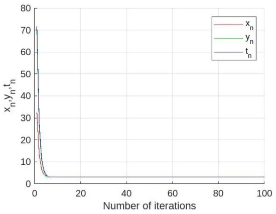
Using the algorithm described above, we obtain the numerical result for approximating the value of π, which is presented in Figure 1 and Table 1 below, where $x_1$ and u are obtained by randomly selecting initial values from the interval $[\pi -100]$ and $n=N=100.$

Figure 1. The convergence of $\left\{x_n\right\},\left\{y_n\right\}$, and $\left\{t_n\right\}$ with Theorem 1.

Table 1. The numerical results of $\left\{x_n\right\},\left\{y_n\right\}$, and $\left\{t_n\right\}$ of Theorem 1.

n	$\left\{{\mathit{x}}_{\mathit{n}}\right\}$	$\left\{{\mathit{y}}_{\mathit{n}}\right\}$	$\left\{{\mathit{t}}_{\mathit{n}}\right\}$
1	32.492625	69.670600	71.627335
2	13.332923	26.622419	27.600786
3	6.767308	10.968535	11.946902
4	4.342317	6.076696	6.076696
5	3.540187	3.141593	4.119960
6	3.141593	3.141593	3.141593
⋮	⋮	⋮	⋮
98	3.141593	3.141593	3.141593
99	3.141593	3.141593	3.141593
100	3.141593	3.141593	3.141593
Time taken (s)	0.066431

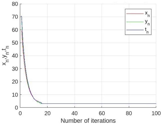
Next, we use ${\alpha }_n={\displaystyle \frac{n}{5n+2}}$ and ${\lambda }_n={\displaystyle \frac{1}{6}}$ for algorithm 1 in [12]. Define the mapping $T=I-{\displaystyle \frac{h}{h^{\prime }}}$ with h the same as h in Example 2 and define the bifunction $f:C\times C\to \mathbb{R}$ by

$$f(x,y)=⟨x,2(y-x)⟩,\forall x,y\in C.$$

We derive the numerical result for approximating the value of π, which is presented in Figure 2 and Table 2 below, where $x_1$ is obtained by randomly selecting initial values from the interval $[\pi -100]$ and $n=N=100.$

Figure 2. The convergence of $\left\{x_n\right\},\left\{y_n\right\}$, and $\left\{t_n\right\}$ with algorithm 1 in [12].

Table 2. The numerical results of $\left\{x_n\right\},\left\{y_n\right\}$, and $\left\{t_n\right\}$ of algorithm 1 in [12].

n	$\left\{{\mathit{x}}_{\mathit{n}}\right\}$	$\left\{{\mathit{y}}_{\mathit{n}}\right\}$	$\left\{{\mathit{t}}_{\mathit{n}}\right\}$
1	59.453602	68.692232	70.648967
2	44.630186	49.124877	51.081612
3	34.095786	37.384464	38.362832
4	26.432642	28.579154	29.557522
5	20.679502	21.730580	22.708948
⋮	⋮	⋮	⋮
11	6.140857	6.076696	6.076696
12	5.309682	5.098328	5.098328
13	4.821363	4.119960	5.098328
14	4.333553	4.119960	4.119960
15	4.046054	3.141593	4.119960
16	3.141593	3.141593	3.141593
⋮	⋮	⋮	⋮
98	3.141593	3.141593	3.141593
99	3.141593	3.141593	3.141593
100	3.141593	3.141593	3.141593
Time taken (s)	0.084881

6. Conclusions

In this work, we present a novel method for the extragradient algorithm to find a common element between the set of fixed points of nonexpansive mappings and the set of solutions to equilibrium problems for a pseudomonotone, Lipschitz-type continuous bifunction. We obtain some strong convergence theorems for the sequence generated by the proposed algorithm under suitable conditions. However, we would like to remark the following:

(1)

Our result is proved without the assumption ${\displaystyle \underset{n\to \infty }{lim}\parallel x_{n+1}-x_n\parallel =0}$ (there are many researchers who have proved strong convergence theorems with this assumption; see [12,13,14]).

(2)

In Theorem 2, we use (34) instead of ${\displaystyle \sum _{i=1}^N{a}_i{f}_i(x_n,y)}$ in (3) and prove the strong convergence theorem, which is applied to effectively solve the combination of variational inequality problem (CVIP).

(3)

In Corollary 1, we use $\nabla {\Im }_i$ in (36) instead of the mapping $A_i$ in Theorem 2, where $i=1,2,3,...,N,$ and prove the strong convergence theorem, which is applied to the standard constrained convex optimization problem.

(4)

We provide Example 1 to demonstrate the efficiency and implementation of our main result in the space $l_2\left(\mathbb{R}\right)$. The convergence of $\left\{x_n\right\},\left\{y_n\right\}$, and $\left\{t_n\right\}$ in Example 1 is guaranteed by Theorem 1.

(5)

In Example 2, we obtain a numerical result for approximating the value of $\pi$, which is presented in Figure 2 and Table 2. Moreover, we obtain the numerical comparison between our algorithm and algorithm 1 in [12], showing that the sequences $\left\{x_n\right\},\left\{y_n\right\}$, and $\left\{t_n\right\}$ of our algorithm converge faster than the sequences $\left\{x_n\right\},\left\{y_n\right\}$, and $\left\{t_n\right\}$ of algorithm 1 in [12].

References

- Ansari, Q.H.; Al-Homidan, S.; Yao, J.C. Equilibrium Problems and Fixed Point Theory. Fixed Point Theory Appl. 2012, 2012, 25. [Google Scholar] [CrossRef][Green Version]
- Farid, M. Two algorithms for solving mixed equilibrium problems and fixed point problems in Hilbert spaces. Ann. Univ. Ferrara 2021, 67, 253–268. [Google Scholar] [CrossRef]
- Latif, A.; Eslamian, M. A New Iterative Method for Equilibrium Problems and Fixed Point Problems. Nonlin. Anal. Geom. Funct. Theory 2013, 2013, 178053. [Google Scholar] [CrossRef][Green Version]
- Cheawchan, K.; Kangtunyakarn, A. The modified split generalized equilibrium problem for quasi-nonexpansive mappings and applications. J. Inequal. Appl. 2018, 122, 1–28. [Google Scholar] [CrossRef] [PubMed]
- Suwannaut, S.; Kangtunyakarn, A. On Approximation of the Combination of Variational Inequality Problem and Equilibrium Problem for Nonlinear Mappings. Thai J. Math. 2021, 19, 1477–1498. [Google Scholar]
- Takahashi, S.; Takahashi, W. Viscosity approximation methods for equilibrium problems and fixed point problems in Hilbert space. J. Math. Anal. Appl. 2007, 331, 506–515. [Google Scholar] [CrossRef]
- Censor, Y.; Gibali, A.; Reich, S. Algorithms for the split variational inequality problem. Numer. Algorithms 2012, 59, 301–323. [Google Scholar] [CrossRef]
- Ceng, L.C.; Yao, J.C. Iterative algorithm for generalized set-valued strong nonlinear mixed variational-like inequalities. J. Opt. Theory Appl. 2005, 124, 725–738. [Google Scholar] [CrossRef]
- Sripattanet, A.; Kangtunyakarn, A. Approximation of G-variational inequality problems and fixed-point problems of G-κ-strictly pseudocontractive mappings by an intermixed method endowed with a graph. J. Inequal. Appl. 2023, 2023, 63. [Google Scholar] [CrossRef]
- Yao, Y.; Yao, J.C. On modified iterative method for nonexpansive mappings and monotone mappings. Appl. Math. Comput. 2007, 186, 1551–1558. [Google Scholar] [CrossRef]
- Peng, J.W. Iterative algorithms for mixed equilibrium problems, strict pseudocontractions and monotone mappings. J. Optim. Theory Appl. 2010, 144, 107–119. [Google Scholar] [CrossRef]
- Pham, P.N. A hybrid extragradient method extended to fixed point problems and equilibrium problems. Optimization 2013, 62, 271–283. [Google Scholar] [CrossRef]
- Zeng, L.C.; Yao, J.C. Strong convergence theorem by an extragradient method for fixed point problems and variational inequality problems. Taiwan. J. Math. 2006, 10, 1293–1303. [Google Scholar] [CrossRef]
- Muangchoo, K. A new explicit extragradient method for solving equilibrium problems with convex constraints. Nonlinear Funct. Anal. Appl. 2022, 27, 1–22. [Google Scholar] [CrossRef]
- Facchinei, F.; Pang, J.S. Finite-Dimensional Variational Inequalities and Complementary Problems; Springer: New York, NY, USA, 2003. [Google Scholar]
- Mainge, P.E. Strong convergence of projected subgradient methods for nonsmooth and nnonstrictly convex minimization. Set-Valued Anal. 2008, 16, 899–912. [Google Scholar] [CrossRef]
- Du, W.S.; He, Z. Feasible iterative algorithms for split common solution problems. J. Nonlinear Convex Anal. 2015, 16, 697–710. [Google Scholar]
- Xu, H.K. Iterative algorithm for nonlinear operators. J. Lond. Math. Soc. 2002, 2, 1–17. [Google Scholar] [CrossRef]
- Kheawborisut, A.; Kangtunyakarn, A. Modified subgradient extragradient method for system of variational inclusion problem and finite family of variational inequalities problem in real Hilbert space. J. Inequal. Appl. 2021, 2021, 53. [Google Scholar] [CrossRef]
- Su, M.; Xu, H.K. Remarks on the Gradient-Projection Algorithm. J. Nonlinear Anal. Optim. 2010, 1, 35–43. [Google Scholar]
Disclaimer/Publisher’s Note: The statements, opinions and data contained in all publications are solely those of the individual author(s) and contributor(s) and not of MDPI and/or the editor(s). MDPI and/or the editor(s) disclaim responsibility for any injury to people or property resulting from any ideas, methods, instructions or products referred to in the content. |
© 2024 by the authors. Licensee MDPI, Basel, Switzerland. This article is an open access article distributed under the terms and conditions of the Creative Commons Attribution (CC BY) license (https://creativecommons.org/licenses/by/4.0/).