Positivity-Preserving Rational Cubic Fractal Interpolation Function Together with Its Zipper Form

Abstract

In this paper, a novel class of rational cubic fractal interpolation function (RCFIF) has been proposed, which is characterized by one shape parameter and a linear denominator. In interpolation for shape preservation, the proposed rational cubic fractal interpolation function provides a simple but effective approach. The nature of shape preservation of the proposed rational cubic fractal interpolation function makes them valuable in the field of data visualization, as it is crucial to maintain the original data shape in data visualization. Furthermore, we discussed the upper bound of error and explored the mathematical framework to ensure the convergence of RCFIF. Shape parameters and scaling factors are constraints to obtain the desired shape-preserving properties. We further generalized the proposed RCFIF by introducing the concept of signature, giving its construction in the form of a zipper-rational cubic fractal interpolation function (ZRCFIF). The positivity conditions for the rational cubic fractal interpolation function and zipper-rational cubic fractal interpolation function are found, which required a detailed analysis of the conditions where constraints on shape parameters and scaling factor lead to the desired shape-preserving properties. In the field of shape preservation, the proposed rational cubic fractal interpolation function and zipper fractal interpolation function both represent significant advancement by offering a strong tool for data visualization.

1. Introduction

Interpolation is the process of finding the value of a function at a point from its neighboring points, or it is a method for generating new data points within the range of a discrete set of known data points. In numerous areas of scientific computation, especially computer graphics, the science of biology and physical science, and the field of geology and numerical computation, interpolation techniques are necessary, specifically when it comes to repeatedly visualizing discrete data. In the field of science and engineering, visualizing discrete scientific data in continuous form is crucial. Based on their graphical representation, the collected data from any experiment are broadly categorized as positive, monotonic, concave, complex, or constrained by their combination, curve, and surface. For example, in chemical experiments, the quantity of obtained product is always positive, and in the case of metals, the resistivity with temperature monotonically increases in nature. Also, with a certain given initial angle and velocity, the trajectory of a projectile is always concave, and in the case of alternating current, the amplitude during some specific time interval shows both concave and convex properties. For representing discrete data as a continuous curve, splines have proven to be extremely valuable. For the initial development of spline theory for various types of data polynomial splines studied, see [1,2,3,4].

Classical interpolants are suitable for approximating functions with irregular data sets because some of the derivatives of classical interpolants are globally smooth, and some are piecewise; however, it is not possible to preserve the hidden shape properties of the data. This is why it is not an ideal method for designing irregular curves and surfaces. When non-desirable oscillations occur, like a pendulum’s motion on a cart placed in an electrochemical system [5] or a spherical ball falling in a hot micellar solution [6], the observed results are extremely misguided, violating the inherited nature of the data; meanwhile, fractal interpolations are ideal methods for irregularity. Apart from the theoretical significance of fractal interpolation, fractal interpolation has a self-similarity property and the ability to possess fractality in the functions or their respective derivatives, which helps them to approximate nonlinear phenomena accurately. Fractal interpolation is an advanced and modern technique that can be used to analyze numerous scientifically obtained data from some scientific phenomena and unknown complicated functions. Fractal interpolation not only helps construct rough structures but also ensures that smooth structures can be constructed. Depending on the values of parameters of iterated function systems, such structures can have a non-integer dimension [7,8,9].

The word “fractal” was coined by the mathematician Mandelbrot in 1975 to describe sophisticated and irregular natural objects and to better understand some scientific experiments that have the presence of self-similarity. The roots of fractal theory began to form in the 17th century when Leibniz mistakenly considered the case that self-similarity only occurs in straight lines. Karl Weierstrass, on 18 July 1872, presented a paper in which he gave the first definition for a function that was continuous everywhere but differentiable nowhere. Soon afterward, Georg Cantor, in 1883, presented examples of a subset of the real line, known as the Cantor set, which had some irregular properties that made it a fractal. At the end of that century, Henri Poincare and Felix Klein introduced another type of fractal, known as a self-inverse fractal. In 1904, Helge Von Koch extended Poincare’s idea and was also not satisfied with the abstract and analytic definition given by Weierstrass. He presented a definition that was more geometric, along with a hand drawn image of such a function; these functions are now known as Koch snowflakes. Wacław Sierpinski made his contribution in 1915 by presenting the triangle and carpet. The fractal interpolation function was presented by Barnsley [8,10] in 1986. There, he introduced a real-valued interpolation function, which was defined on a compact interval of R. This function works well with objects that are present in nature, with some geometrical self-similarity. Ever since, fractal interpolation has been attracting more attention, as it can be used in almost every field of life science, including medicine, visualization, engineering science, finance, and other areas. Fractal interpolation has a wide area of use in the real world; it is used in movies, medical science, image compression, etc. Knowledge of fractals and ecosystems together is used to determine the acidrain spread of smoke. The best method to construct the fractal interpolation function is using the theory of IFS [11]. Harrington [12] introduced the k-times differentiable fractal interpolation function (FIF). The smooth FIF [13] was shown by Navascués in 2006. Many researchers have worked on shape-preserving smooth FIFs since they are useful in many scientific and economic areas such as medicine, stock markets, etc. Rational splines are one of the most used shape-preserving interpolants as they are more flexible [14,15,16,17,18]. M. A. Navascués introduced the concept of $\alpha$ fractal function [19], and M. Nasim Akhtar, together with M. A. Navascués [20], introduced the local non-affine $\alpha$ fractal interpolation function. In recent years, many authors have worked on different areas of fractal theory, such as fractal dimensions and fractal surfaces [21,22,23,24,25,26,27,28]. Recently, Bilel Selmi discussed the dimension of fractal functions on the product of the Sierpinski gasket [29]. M. A. Navascués [30] discussed a new type of contraction and the existence and uniqueness theorem of this map. In Ref. [31], the fractal interpolation function using the Kannan contraction is discussed, and the generation of fractals using the IFS of the Kannan contraction in a controlled metric space is presented in [32].

Shape preservation is one of the most important properties of fractal interpolation. The geometrical characteristics of the interpolating data are maintained using shape preservation. Shape preservation involves three key properties of functions: positivity, monotonicity, and convexity. All these three properties are essential in numerous real-world applications as they can define or maintain the curvature and nature of functions or data within their domain. Positivity is important in various real-world applications, including physical quantities such as mass, length, probability distributions, time series analysis, and more. The positivity of various classical and fractal interpolation functions has been discussed in the literature. For detailed studies, see [33,34,35,36,37] and the references therein. Similarly, monotonicity is another crucial property. This property ensures that the function follows a consistent trend (non-decreasing or non-increasing). Monotonicity is useful in preserving the trend and order of functions or data, which is crucial in maintaining the integrity of time series data and other applications. The monotonicity of various classical and fractal interpolation functions has been discussed in the literature; for detailed studies, see [38,39,40] and the references therein. The convexity is also equally crucial for many real-world applications, such as in the stock market. It helps in predicting market trends and behavior. The convexity property ensures that the function maintains a specific smoothness in the shape of the function or data. The convexity of various classical and fractal interpolation functions has been discussed in the literature; for detailed studies, see [41,42,43,44] and the references therein.

Basic constructions of the zipper have been reported [45,46]. The fractal interpolation functions using the zipper provide greater flexibility due to the presence of a binary vector, also known as a signature. Sangita Jha discussed the zipper quadratic fractal interpolation function and its positivity [47]. They also ensured that the discussed function is non-negative in the defined interval. Vijay and Chand [48] proposed the zipper fractal interpolation function considering variable scaling. By considering variable scaling, one can enhance the adaptability of the function. The convexity of the zipper cubic fractal interpolation function with a quadratic denominator has been discussed by Vijay and Chand [49]. In this paper, we present the construction of a zipper-rational cubic fractal interpolation function. Interpolation with constrained data has a wide application in real-world applications, such as removing undesired wiggles in prominent lines of automobile roofs, in engineering, preventing oscillations between points, and more.

The aim of this paper is to construct a family of shape-preserving rational cubic fractal interpolation functions, including their zipper form, and to demonstrate their advantage over the classical interpolation functions. The qualitative features of an interpolant curve depend mainly on the scaling factor and shape parameters. The constrained RCFIF is designed to ensure that it lies above the straight line for all real values that share this characteristic. This paper is organized as follows: In the Section 2, we provide a short review of the fractal interpolation function (FIF) and the zipper fractal interpolation function (ZFIF). First, we discussed the fundamental concepts and mathematical construction of the fractal interpolation function, along with its uniqueness and existence theorems. This section also highlights the difference between classical interpolation functions and fractal interpolation functions. Then, we discuss the zipper fractal interpolation function, including its basic construction and the presence of a signature, which enhances the flexibility of the interpolating function or data. In the Section 3, we present the construction of the rational cubic fractal interpolation function, and the zipper-rational cubic fractal interpolation function. For the rational cubic fractal interpolation function, we consider a rational function of the form ${\displaystyle \frac{u_j(\theta )}{v_j(\theta )}}$, while for zipper-rational cubic fractal interpolation, the rational function is ${\displaystyle \frac{u_{j,\epsilon }(\theta )}{v_{j,\epsilon }(\theta )}}$, where the numerator is a cubic polynomial, and the denominator is a linear polynomial with one shape parameter. In the Section 4, we discuss the convergence of the rational cubic fractal interpolation function and the zipper-rational cubic fractal interpolation function regarding the data-generating function. Their respective theorems are given with proofs. The convergence analysis includes the error bound and conditions that guarantee the precision and reliability of the considered interpolant. In the Section 5, we constrain the RCFIF and ZRCFIF so that they lie above the straight line. In the Section 6, sufficient conditions are met to obtain the positivity conditions for the rational cubic fractal interpolation function and zipper-rational cubic fractal interpolation function. We derive the mathematical framework to provide the necessary and sufficient conditions for the function to be non-negative. To support the theoretical part, we provide an example with graphical representations. The respective theorems for providing sufficient conditions for the rational cubic fractal interpolation function and zipper-rational cubic fractal interpolation function to be positive are discussed. In the Section 7, we conclude the work done in previous sections and discuss their results. We also suggest potential future work in this area, which can be done by extending the given function to higher-order dimensions and other possible extensions.

2. Basics of Fractal Interpolation Functions and Zipper Fractal Interpolation Functions

In this section, we provide a short review of fractal interpolation functions (FIFs) and zipper fractal interpolation functions (ZFIFs) together with their fundamental equation and uniqueness and existence theorems. First, we discuss the fundamental concepts and mathematical construction of the fractal interpolation function. This section also highlights the difference between classical interpolation functions and fractal interpolation functions. Then, we discuss the zipper fractal interpolation function, including its basic construction and the presence of a signature, which enhances the flexibility of the interpolating function or data.

2.1. Fractal Interpolation Function

Let $\left\{(y_m,z_m)\in J\times K,m\in M_M=1,2,3\dots M\right\}$ be the dataset, where $K$ is a compact set of $R$ and $J=[y_1,y_M]$ satisfying $y_1<y_2<y_3\dots <y_M$ and $J_j=[y_j,y_{j+1}]$ for $j\in M_{M-1},$ $M_{M-1}=1,2,\dots ,M-1$. Consider $L_j:J\to J_j$ the contractive homomorphism defined as $L_j(y)=a_{j}y+b_j$ such that $\forall$$y,y*\in J$ and for some $0\le {\mathcal{l}}_j<1$.

$$\left|L_j(y)-L_j(y*)\right|\le {\mathcal{l}}_j\left|y-y*\right|;L_j(y_1)=y_j,L_j(y_M)=y_{j+1},j\in M_{M-1}$$

(1)

Define $F_j:K:=J\times \left[c,d\right]\to R$ such that, for and let ${\delta }_j\in \left(-1,1\right),$

$$F_j(y,z)-F_j\left(y,z\right)\le \left|{\delta }_j\right|\left|z-z*\right|;F_j\left(y_1,z_1\right)=z_j,F_j\left(y_M,z_M\right)=z_{j+1},j\in M_{M-1}$$

(2)

Now construct a function

$${\mu }_j:J\times R\to J_j\times R,$$

$${\mu }_j(y,z)=(L_j(y),F_j(y,z)),j\in M_{M-1}.$$

Theorem 1

(see [8,10]). The iterated function system  $\left\{J\times K;{\mu }_j,j\in M_{M-1}\right\}$ possesses a unique attractor $H,$ which is also the graph of the continuous function $g’:J\to R$ that satisfies $g’(y_j)=z_j\forall j.$

The above function $g’$ is known as the fractal interpolation function corresponding to the IFS $\left\{J\times K;{\mu }_j,j\in M_{M-1}\right\}$. The most widely studied fractal interpolations and their applications are taken from the following iterated function system:

$$\left\{J\times K;{\mu }_j\left(y,z\right)=\left(L_j\left(y\right),F_j\left(y,z\right)\right);j\in M_{M-1}\right\}$$

(3)

$L_j\left(y\right)=a_{j}y+b_j,F_j\left(y,z\right)={\delta }_{j}z+Q_j\left(y\right)$, where $Q_j:J\to R$ is a continuous function. The multiplier ${\delta }_j$ is known as the vertical scaling factor of a continuous map ${\mu }_j$.

Let $C^r\left(J\right)$ be the collection of all $r$-times continuously differentiable real-valued functions on $J.$ The differentiable fractal interpolation functions are given by the following theorem:

Theorem 2

[12]. Let $\left\{(y_m,z_m)\in J\times K:m=1,2,\dots ,M\right\}$ be the dataset, where $y_1<y_2<\dots <y_M$. Let $L_j\left(y\right)=a_{j}y+b_j,F_j\left(y,z\right)={\delta }_{j}z+Q_j\left(y\right)$, where $Q_j$ is a continuous function for $j\in M_{M-1}$. Suppose that for some integer r $q\ge 0$, $\left|{\delta }_j\right|<a_j^q,j\in M_{M-1}$. Let $F_{j,r}\left(y,z\right)={\displaystyle \frac{{\delta }_{j}z+Q_j^{\left(r\right)}\left(y\right)}{a_j^r}}$, $Q_j^{\left(r\right)}\left(y\right)$ be the rth derivative of $Q_j\left(y\right)$

$$z_{1,r}={\displaystyle \frac{Q_1^{\left(r\right)}\left(y_1\right)}{a_1^r-{\delta }_1}},z_{M,k}={\displaystyle \frac{Q_{M-1}^{\left(r\right)}\left(y_M\right)}{a_{M-1}^{\left(r\right)}-{\delta }_{M-1}}},r=1,2,\dots ,q.$$

If $F_{j-1,r}\left(y_M,z_{M,r}\right)=F_{j,r}\left(y_1,z_{1,r}\right)$ for $j\in M_{M-2} \& r=1,2,\dots ,q$ then a fractal interpolation function $g’$ is determined by an iterated function system $\left\{J\times K;{\mu }_j\left(y,z\right)=\left(L_j\left(y\right),F_j\left(y,z\right)\right),j\in M_{M-1}\right\}$ and the fractal interpolation function $g{’}^{\left(r\right)}\in C^q\left[y_1,y_M\right]$ is determined by an iterated function system $\left\{J\times K,{\mu }_j\left(y,z\right)=\left(L_j\left(y\right),F_{j,r}\left(y,z\right)\right),j\in M_{M-1}\right\}$.

2.2. Zipper Fractal Interpolation Function

In this subsection, we review the construction of the zipper IFS for a given data set. First, we recall the definition of a zipper.

Definition 1.

Consider a non-surjective map   ${\mu }_j,j\in M_{M-1}$ on a complete metric space $\left(X,d\right)$. Then, the system $\Im =\left\{X;{\mu }_j:j\in M_{M-1}\right\}$ is known as the zipper-iterated function system with the vertices $\left(v_1,v_2,\dots ,v_M\right)$ and a signature $\epsilon =\left({\epsilon }_1,{\epsilon }_2,\dots ,{\epsilon }_m\right)\in {\left\{0,1\right\}}^{M-1},$ if ${\mu }_j$ satisfies ${\mu }_j\left(v_1\right)=v_{j+{\epsilon }_j},{\mu }_j\left(v_M\right)=v_{j+1-{\epsilon }_j}$ $\forall j\in M_{M-1}$. Let $B\subset X$ be any compact set satisfying the self-referential equation 

$$B={\displaystyle {\cup }_{j=1}^{M-1}{\mu }_j\left(B\right)}$$

This is known as the attractor corresponding to the zipper IFS $\Im$. The definition of IFS with vertices $\left(v_1,v_2,\dots ,v_M\right)$ and the definition of zipper IFS coincide if we take the signature vector ${\epsilon }_j=0\hspace{0.17em}j\in M_{M-1}$. The following review of the zipper fractal interpolation function is based on [10,46,50].

Let $\left\{\left(y_m,z_m\right)\in J\times R,m\in M_M\right\}$ be the dataset with $y_1<y_2<\dots <y_M$. Consider $J=[y_1,y_M]$ $\&$ $J_j=[y_j,y_{j+1}],j\in M_{M-1}$. Let $L_j:J\to J_j$ the affine map given by $L_j(y)=a_{j}y+b_j,j\in M_{M-1}$ such that

$$L_j(y_1)=y_{j+{\epsilon }_j},L_j(y_M)=y_{j+1-{\epsilon }_j}$$

(4)

$$a_j={\displaystyle \frac{y_{j+1-{\epsilon }_j}-y_{j+{\epsilon }_j}}{y_M-y_1}},b_j={\displaystyle \frac{y_M{y}_{j+{\epsilon }_j}-y_1{y}_{j+1-{\epsilon }_j}}{y_M-y_1}}.$$

Let $j\in M_{M-1},$ $F_j:K:=J\times \left[c,d\right]\to R$ be a function defined as 

$$F_j(y,z)={\delta }_{j}z+Q_j(y)$$

where $Q_j:J\to R$ is the continuous function and ${\delta }_j$ be the vertical scaling factor such that ${\left|\delta \right|}_{\infty }=\max \left\{\left|{\delta }_j\right|:j\in M_{M-1}\right\}<1$, and the following condition holds: 

$$F_j(y_1,z_1)=z_{j+{\epsilon }_j},F_j(y_M,z_M)=z_{j+1-{\epsilon }_j},j\in M_{M-1}.$$

(5)

Now, define a map ${\mu }_j:K\to J_j\times R,j\in M_{M-1}$ as

$${\mu }_j\left(y,z\right)=\left(L_j\left(y\right),F_j\left(y,z\right)\right)\forall \left(y,z\right)\in K.$$

The system $\Im =\left\{K;{\mu }_j,j\in M_{M-1}\right\}$ is a zipper-iterated function system with vertices $\left\{\left(y_m,z_m\right),m\in M_M\right\}$ and a signature $\epsilon =\left({\epsilon }_1,{\epsilon }_2,\dots ,{\epsilon }_{M-1}\right)$. The construction of Zipper-FIF is presented in the following theorem from [51].

Theorem 3.

The following conditions hold for the IFS $\left\{K;{\mu }_j,j\in M_{M-1}\right\}$

• There is a unique compact set $H\subset K$ such that $H={\displaystyle {\cup }_{j=1}^{M-1}{\mu }_j\left(H\right).}$
• The continuous function $g_{\epsilon }^{\delta }:J\to R$ that interpolates the dataset $\{(y_m,z_m)\in J\times R:m\in M_M\}$, i.e., $H=\left\{\left(y,g_{\epsilon }^{\delta }\left(y\right)\right):y\in J\right\} \& g_{\epsilon }^{\delta }\left(y_j\right)=z_j\forall j.$

3. Construction of Rational Cubic Fractal Interpolation Function and Zipper-Rational Cubic Fractal Interpolation Function

This section is divided into two parts. In the first subsection, we discuss the construction of the rational cubic fractal interpolation function, and in the second, we discuss the construction of the zipper-rational cubic fractal interpolation function:

3.1. C¹—Rational Cubic Fractal Interpolation Function

In this subsection, we provide the construction of the rational cubic fractal interpolation function with one shape parameter. Let $\left\{\left(y_m,z_m\right)\in J\times K;m\in M_M\right\}$ be the given set of data for an original function $\phi$ such that $y_1<y_2<\dots <y_M$. Let $\left\{J\times K;{\mu }_j\left(y,z\right)=\left(L_j\left(y\right),F_j\left(y,z\right)\right)\forall j\in M_{M-1}\right\}$ be the IFS, where $L_j\left(y\right)=a_{j}y+b_j,$ $F_j\left(y,z\right)={\delta }_{j}z+Q_j\left(y\right)$, $Q_j\left(y\right)={\displaystyle \frac{u_j\left(y\right)}{v_j\left(y\right)}}$, $u_j\left(y\right)$ is a cubic polynomial and $v_j\left(y\right)$ is a linear polynomial, $v_j\left(y\right)\ne 0\forall y\in J$, $\left|{\delta }_j\right|<a_j,j\in M_{M-1}$. Let

$$F_j^{\left(1\right)}\left(y,d\right)={\displaystyle \frac{{\delta }_{j}d+Q_j^{\left(1\right)}\left(y\right)}{a_j}},$$

where $Q_j^{\left(1\right)}\left(y\right)$ is the first-order derivative of $Q_j\left(y\right)$, $y\in \left[y_1,y_M\right]$. The following join-up conditions are satisfied by $F_j\left(y,S^{\delta }\right)$

$$\begin{array}{l}{F}_j\left(y_1,S_1^{\delta }\right)=z_j,F_j\left(y_M,S_M^{\delta }\right)=z_{j+1},\\ F_j^{\left(1\right)}\left(y_1,d_1\right)=d_j,F_j^{\left(1\right)}\left(y_M,d_M\right)=d_{j+1},\end{array}$$

(6)

where $d_j$ is the first-order derivative of $S^{\delta }$ regarding $y$ at knot $y_j$. The attractor obtained by the above-iterated function system will be the graph of the $C^1$-rational cubic fractal interpolation function. Now, from (3), it can be observed that the FIF can be written as:

$$S^{\delta }\left(L_j\left(y\right)\right)={\delta }_j{S}^{\delta }\left(y\right)+Q_j\left(y\right)={\delta }_j{S}^{\delta }\left(y\right)+{\displaystyle \frac{u_j\left(\theta \right)}{v_j\left(\theta \right)}},$$

(7)

$$u_j\left(\theta \right)=A{\left(1-\theta \right)}^3+B{\left(1-\theta \right)}^2\theta +C\left(1-\theta \right){\theta }^2+D{\theta }^3,$$

$$v_j\left(\theta \right)=1+s_j\left(1-\theta \right),\theta ={\displaystyle \frac{y-y_1}{l}},l=y_M-y_1\forall y\in J,$$

and $s_j$ is a positive shape parameter. The following conditions are imposed to ensure that the rational cubic fractal interpolation function is $C^1$-continuous:

$$\begin{array}{l}{S}^{\delta }\left(L_j\left(y_1\right)\right)=z_j,S^{\delta }\left(L_j\left(y_M\right)\right)=z_{j+1},\\ {\left(S^{\delta }\right)}^{\prime }\left(L_j\left(y_1\right)\right)=d_j,{\left(S^{\delta }\right)}^{\prime }\left(L_j\left(y_M\right)\right)=d_{j+1},j\in M_{M-1}.\end{array}$$

(8)

From Equations (7) and (8), it is evident that if we take $y=y_1$ in Equation (7), then we obtain

$$S^{\delta }\left(L_j\left(y_1\right)\right)=z_j\Rightarrow z_j={\delta }_j{z}_1+{\displaystyle \frac{A}{1+s_j}}\Rightarrow A=\left(1+s_j\right)\left(z_j-{\delta }_j{z}_1\right).$$

Similarly, to calculate the value of $D$, if we take $y=y_M$ in Equation (7), then we obtain

$$S^{\delta }\left(L_j\left(y_M\right)\right)=z_{j+1}\Rightarrow z_{j+1}={\delta }_j{z}_M+{\displaystyle \frac{D}{1}}\Rightarrow D=z_{j+1}-{\delta }_j{z}_M.$$

Differentiate Equation (7) with respect to the y,

$${\left(S^{\delta }\right)}^{\left(1\right)}\left(L_j\left(y\right)\right)L_j{ }^{\left(1\right)}\left(y\right)={\delta }_j{\left(S^{\delta }\right)}^{\left(1\right)}\left(y\right)+Q_j{ }^{\left(1\right)}\left(y\right)$$

Now, to calculate the value of $B$, if we take $y=y_1$ in ${\left(S^{\delta }\right)}^{\prime }\left(L_j\left(y\right)\right)$ and use Equation (8), we obtain

$$\Rightarrow B=\left(3+2s_j\right)\left(z_j-{\delta }_j{z}_1\right)+l_j\left(1+s_j\right)\left(a_j{d}_j-{\delta }_j{d}_1\right)$$

Similarly, to calculate the value of $C$, take $y=y_M$ in ${\left(S^{\delta }\right)}^{\prime }\left(L_j\left(y\right)\right)$ and use Equation (8). Then, we have

$${\left(S^{\delta }\right)}^{\prime }\left(L_j\left(y_M\right)\right)=d_{j+1}\Rightarrow a_j{d}_{j+1}={\delta }_j{d}_M+{\displaystyle \frac{\left(-C+3D\right)-D\left(-s_j\right)}{l_j}}$$

$$\Rightarrow C=\left(3+s_j\right)\left(z_{j+1}-{\delta }_j{z}_M\right)-l_j\left(a_j{d}_{j+1}-{\delta }_j{d}_M\right)$$

Now, by substituting the values of $A,B,C \& D$ into Equation (7), we obtain the required well-defined $C^1$-rational cubic fractal interpolation function, whose numerator is:

$$\begin{array}{l}{u}_j\left(\theta \right)=\left(1+s_j\right)\left(z_j-{\delta }_j{z}_1\right){\left(1-\theta \right)}^3+\left\{\left(3+2s_j\right)\left(z_j-{\delta }_j{z}_1\right)+l_j\left(1+s_j\right)\left(a_j{d}_j-{\delta }_j{d}_1\right)\right\}{\left(1-\theta \right)}^2\theta \\ +\left\{\left(3+s_j\right)\left(z_{j+1}-{\delta }_j{z}_M\right)-l_j\left(a_j{d}_{j+1}-{\delta }_j{d}_M\right)\right\}\left(1-\theta \right){\theta }^2+\left(z_{j+1}-{\delta }_j{z}_M\right){\theta }^3.\end{array}$$

The derivatives $d_m,m\in M_M$ can be calculated either using numerical methods or from the given set of data if it is not given. We calculated it using the arithmetic mean method on a given set of data.

Remark 1.

If ${\delta }_j=0$, then the rational cubic fractal interpolation function will be reduced to the rational cubic interpolant, which is of the form

$$S\left(y\right)={\displaystyle \frac{u_j^{*}\left(t\right)}{v_j^{*}\left(t\right)}},y\in \left[y_j,y_{j+1}\right],$$

(9)

with

$$\begin{array}{l}{u}_j^{*}\left(t\right)=\left(1+s_j\right)z_j{\left(1-t\right)}^3+\left\{\left(3+2s_j\right)z_j+{\hslash }_j\left(1+s_j\right)d_j\right\}{\left(1-t\right)}^{2}t+\left\{\left(3+s_j\right)z_{j+1}-{\hslash }_j{d}_{j+1}\right\}\\ \left(1-t\right)t^2+z_{j+1}{t}^3,v_j^{*}\left(t\right)=1+s_j\left(1-t\right),t={\displaystyle \frac{y-y_1}{y_M-y_1}},y\in J\end{array}$$

Example 1.

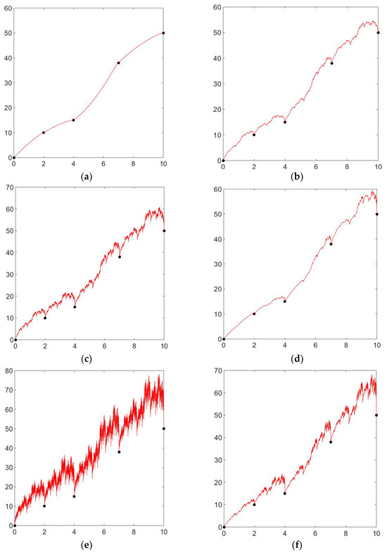
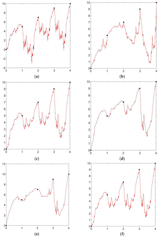
To verify the diversity and flexibility of the rational cubic fractal interpolation function over the classical cubic fractal interpolation function, we provide an example considering the interpolating points $\left(0,0\right),\left(2,10\right),\left(4,15\right),\left(7,38\right),\left(10,50\right)$. Throughout Figure 1, the shape parameter $s_j$ is considered $\left(50,50,50,50\right)$. The rational cubic fractal interpolation function is shown in Figure 1. Now, if we compare the figures with each other, the change is visible and is due to different values of the scaling factor. We have taken different values for each figure. In Figure 1a, we have taken the scaling factor $\delta =\left(0,0,0,0\right)$ and $\delta =\left(0.2,0.25,0.45,0.5\right)$ in Figure 1b, comparing Figure 1a,b, Figure 1a is less detailed, whereas Figure 1b is more detailed and dense due to the increased scaling factor. Similarly, in Figure 1c,d, the scaling factors are $\delta =\left(0.3,0.24,0.6,0.72\right)$ and $\delta =\left(0.04,0.15,0.35,0.75\right)$, respectively. Figure 1d is more basic compared to Figure 1c, where the shape is more filled in and intricate. Figure 1e with scaling factor $\delta =(0.14,0.42,0.56,0.92)$ and Figure 1f with scaling factor $\delta =\left(0.04,0.15,0.35,0.75\right)$ can be compared similarly. In this way, we can compare all these figures based on the scaling factor.

3.2. C¹-Zipper-Rational Cubic Fractal Interpolation Function

In this subsection, we construct the zipper-rational cubic fractal interpolation function:

Consider the zipper-rational iterated function system, where the rational function is

$$Q_{j,\epsilon }\left(y\right)={\displaystyle \frac{u_{j,\epsilon }\left(\theta \right)}{v_{j,\epsilon }\left(\theta \right)}}$$

where

$$u_{j,\epsilon }\left(\theta \right)=A_{j,\epsilon }{\left(1-\theta \right)}^3+B_{j,\epsilon }{\left(1-\theta \right)}^2\theta +C_{j,\epsilon }\left(1-\theta \right){\theta }^2+D_{j,\epsilon }{\theta }^3,$$

$$v_{j,\epsilon }\left(\theta \right)=1+s_j\left(1-\theta \right)$$

For $0\le \theta ={\displaystyle \frac{y-y_1}{y_M-y_1}}\le 1$, $s_j$ is a non-negative shape parameter. Suppose $\tilde{C}\left(J\right)=\left\{g:J\to R,g\left(y_1\right)=z_1,g\left(y_M\right)=z_M\right\}$. Then, $\tilde{C}\left(J\right)$ is the subspace of space $C\left(J\right)$ and $\tilde{C}\left(J\right)$ is complete with respect to the uniform norm. Let ${\epsilon }_j\in {\left\{0,1\right\}}^{M-1}$ be fixed and define the Read–Bajraktarevic (R–B) operator $T_{\epsilon }^{\delta }:\tilde{C}\left(J\right)\to \tilde{C}\left(J\right)$ as:

$$T_{\epsilon }^{\delta }\left(L_j\left(y\right)\right)=F_j\left(y,g\left(y\right)\right)$$

$$={\delta }_{j}g\left(y\right)+{\displaystyle \frac{A_{j,\epsilon }{\left(1-\theta \right)}^3+B_{j,\epsilon }{\left(1-\theta \right)}^2\theta +C_{j,\epsilon }\left(1-\theta \right){\theta }^2+D_{j,\epsilon }{\theta }^3}{1+s_j\left(1-\theta \right)}}$$

$T_{\epsilon }^{\delta }$ is a contraction on complete metric space $\left(\tilde{C}\left(J\right),{‖.‖}_{\infty }\right)$. By the Banach contraction, theorem, $T_{\epsilon }^{\delta }$ possesses a fixed point $S_{\epsilon }^{\delta }$ that satisfies:

$$S_{\epsilon }^{\delta }\left(L_j\left(y\right)\right)={\delta }_j{S}_{\epsilon }^{\delta }\left(y\right)+Q_{j,\epsilon }\left(y\right)$$

(10)

$$={\delta }_j{S}_{\epsilon }^{\delta }\left(y\right)+{\displaystyle \frac{A_{j,\epsilon }{\left(1-\theta \right)}^3+B_{j,\epsilon }{\left(1-\theta \right)}^2\theta +C_{j,\epsilon }\left(1-\theta \right){\theta }^2+D_{j,\epsilon }{\theta }^3}{1+s_j\left(1-\theta \right)}}$$

The coefficients in this expression $Q_{j,\epsilon }\left(y\right)$ can be calculated using conditions given in Equation (2), which is an operation similar to calculating them from the relation $S_{\epsilon }^{\delta }\left(y_j\right)=y_{j+{\epsilon }_j} \& S_{\epsilon }^{\delta }\left(y_{j+1}\right)=y_{j+1-{\epsilon }_j}$. According to [12], for a differentiable fractal interpolation function, the scaling factor is selected as $\left|{\delta }_j\right|<a_j\forall j\in M_{M-1}$. For the construction of the C¹ zipper-rational cubic fractal interpolation function, we need the following interpolating conditions:

$$\begin{gathered} S_{\epsilon }^{\delta }\left(L_j\left(y_1\right)\right)=z_{j+{\epsilon }_j},S_{\epsilon }^{\delta }\left(L_j\left(y_M\right)\right)=z_{j+1-{\epsilon }_j}\& \\ {\left(S_{\epsilon }^{\delta }\right)}^{\left(1\right)}\left(L_j\left(y_0\right)\right)=d_{j+{\epsilon }_j},{\left(S_{\epsilon }^{\delta }\right)}^{\left(1\right)}\left(L_j\left(y_M\right)\right)=d_{j+1-{\epsilon }_j}, \end{gathered}$$

where $d_{j+{\epsilon }_j}$ is the first-order derivative with respect to “y” at knots $y_j$, respectively. To calculate the value of $A_{j,\epsilon }$, take $y=y_1$ in Equation (10) and we obtain

$$A_{j,\epsilon }=\left(1+s_j\right)\left(z_{j+{\epsilon }_j}-{\delta }_j{z}_1\right)$$

Similarly, to calculate the value of $D_{j,\epsilon }$, take $y=y_M$ in Equation (10) and we obtain

$$D_{j,\epsilon }=z_{j+1-{\epsilon }_j}-{\delta }_j{z}_M$$

By taking the first-order derivative of the functional equation, we obtain

$${\left(S_{\epsilon }^{\delta }\right)}^{\left(1\right)}\left(L_j\left(y\right)\right)L_j{ }^{\left(1\right)}\left(y\right)={\delta }_j{\left(S_{\epsilon }^{\delta }\right)}^{\left(1\right)}\left(y\right)+Q_{j,\epsilon }{ }^{\left(1\right)}\left(y\right)$$

to calculate the value of $B_{j,\epsilon }$, take $y=y_1$ in the above equation, and we obtain

$$B_{j,\epsilon }=\left(3+2s_j\right)z_{j+{\epsilon }_j}+\left(1+s_j\right)h_j{d}_{j+{\epsilon }_j}-{\delta }_j\left(\left(3+2s_j\right)z_1+\left(1+s_j\right)\left(y_M-y_1\right)d_1\right)$$

where $h_j=y_{j+1-{\epsilon }_j}-y_{j+{\epsilon }_j}$. Again, to calculate the value of $C_{j,\epsilon }$, taking $y=y_M$ in the above equation, we obtain

$$C_{j,\epsilon }=\left(3+s_j\right)z_{j+1-{\epsilon }_j}-h_j{d}_{j+1-{\epsilon }_j}-{\delta }_j\left(\left(3+s_j\right)z_M-\left(y_M-y_1\right)d_M\right).$$

Thus, we obtain the desired zipper-rational cubic fractal interpolation function, which is

$$S_{\epsilon }^{\delta }\left(L_j\left(y\right)\right)={\delta }_j{S}_{\epsilon }^{\delta }\left(y\right)+{\displaystyle \frac{u_{j,\epsilon }^{\ast }\left(\theta \right)}{v_{j,\epsilon }\left(\theta \right)}}$$

The values of $u_{j,\epsilon }^{\ast }\left(\theta \right)$ and $v_{j,\epsilon }\left(\theta \right)$ are provided below:

$$\begin{array}{l}{u}_{j,\epsilon }\left(\theta \right)\equiv u_{j,\epsilon }^{\ast }\left(\theta \right)=\left(1+s_j\right)\left(z_{j+{\epsilon }_j}-{\delta }_j{z}_1\right){\left(1-\theta \right)}^3+\left(z_{j+1-{\epsilon }_j}-{\delta }_j{z}_M\right){\theta }^3\\ +\left(\left(3+2s_j\right)z_{j+{\epsilon }_j}+\left(1+s_j\right)h_j{d}_{j+{\epsilon }_j}-{\delta }_j\left(\left(3+2s_j\right)z_1+\left(1+s_j\right)\left(y_M-y_1\right)d_1\right)\right){\left(1-\theta \right)}^2\theta \\ +\left(\left(3+s_j\right)z_{j+1-{\epsilon }_j}-h_j{d}_{j+1-{\epsilon }_j}-{\delta }_j\left(\left(3+s_j\right)z_M-\left(y_M-y_1\right)d_M\right)\right)\left(1-\theta \right){\theta }^2,\end{array}$$

$$v_{j,\epsilon }\left(\theta \right)=1+s_j\left(1-\theta \right)$$

Remark 2.

If the signature is ${\epsilon }_m=0$, then the zipper-rational cubic fractal interpolation function reduces to the rational cubic fractal interpolation function

$$S^{\delta }\left(L_j\left(y\right)\right)={\delta }_j{S}^{\delta }\left(y\right)+Q_j\left(y\right),Q_j\left(y\right)={\displaystyle \frac{u_j\left(\theta \right)}{v_j\left(\theta \right)}}$$

(11)

where the values of  $u_j\left(\theta \right)$ and $v_j\left(\theta \right)$ are given in Section 3.1.

Remark 3.

If ${\epsilon }_j=0={\delta }_j$, then the zipper-rational cubic fractal interpolation function reduces to the rational cubic interpolant, discussed in Remark 1 of Section 3.1.

Example 2.

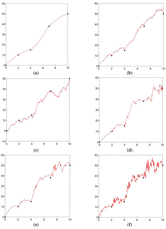
To verify the diversity and flexibility of the zipper-rational cubic fractal interpolation function compared to the rational cubic fractal interpolation function, we provide an example considering the interpolating points $\left(0,0\right),\left(2,10\right),\left(4,15\right),\left(7,38\right),\left(10,50\right)$. Throughout Figure 2, the shape parameter $s_j$ is considered $\left(50,50,50,50\right)$. In Figure 2a, we have taken the scaling factor $\delta =\left(0,0,0,0\right)$ and signature as $\epsilon =\left(0,0,0,0\right)$, and in Figure 2b, the signature as $\epsilon =\left(0,0,0,0\right)$ and scaling factor as $\delta =\left(0.2,0.25,0.45,0.5\right)$. Comparing Figure 2a,b, Figure 2a is less detailed, whereas Figure 2b is more is more detailed and dense due to the increased scaling factor. Since we have taken the signature as $\epsilon =\left(0,0,0,0\right)$, these figures are the same as Figure 1a and Figure 1b. Comparing Figure 2b,c, we have taken the same scaling factor as $\delta =\left(0.2,0.25,0.45,0.5\right)$ for both figures and the signature as $\epsilon =\left(0,0,0,0\right)$ and $\epsilon =\left(1,1,1,0\right)$, respectively, Figure 2c is more detailed or enhanced as it is producing a negative graph due to the change in signature value. Figure 2d,e can be compared as we have taken the same scaling factor $\delta =\left(0.04,0.15,0.35,0.75\right)$ in both figures and signature as $\epsilon =\left(0,1,1,0\right)$ and $\epsilon =\left(1,1,1,1\right)$, respectively. Comparing Figure 2e with scaling factor $\delta =\left(0.04,0.15,0.35,0.75\right)$ and signature as $\epsilon =\left(1,1,1,1\right)$ to Figure 2f with scaling factor $\delta =(0.14,0.42,0.56,0.92)$ and signature as $\epsilon =\left(1,1,1,1\right)$, Figure 2f is more detailed compared to Figure 2e, which is due to the increase in the scaling factor.

The changes in the graphs of Figure 1 and Figure 2 are clearly visible. We have taken the same scaling factor in some of the graphs, but in Figure 2, due to the presence of signature, the curve of function is changed.

4. Convergence of Rational Cubic Fractal Interpolation Function and Zipper-Rational Cubic Fractal Interpolation Function

In this section, we determine the error bounds for uniform distance between the data-generating function $\phi$, which belongs to $C^2\left[y_1,y_M\right]$, and the rational cubic fractal interpolation function. It is difficult to calculate the uniform error bound ${‖\phi -S^{\delta }‖}_{\infty }$ using the standard techniques since the rational cubic fractal interpolation function $S^{\delta }$ has an implicit expression. Hence, we use the classical rational cubic function to drive the upper bound of the uniform error:

$${‖\phi -S^{\delta }‖}_{\infty }\le {‖\phi -S‖}_{\infty }+{‖S-S^{\delta }‖}_{\infty }$$

(12)

To show the convergence of the C¹-zipper-rational cubic fractal interpolation function $S_{\epsilon }^{\delta }$ toward the $\phi$, the data-generating function belongs to $C^2\left[y_1,y_M\right]$. We need to find a uniform distance between them. It will be difficult to calculate ${‖\phi -S_{\epsilon }^{\delta }‖}_{\infty }$ using the standard techniques due to the implicit nature of $S_{\epsilon }^{\delta }$. Let $S_{\epsilon }^{\delta }$ be the C¹ zipper-rational cubic fractal interpolation function and $\phi$ data-generating function, respectively. We will derive an upper bound of the error using $S_{\epsilon }^{\delta }-S^{\delta }$.

By the triangular inequality, we have

$${‖\phi -S_{\epsilon }^{\delta }‖}_{\infty }\le {‖\phi -S^{\delta }‖}_{\infty }+{‖S_{\epsilon }^{\delta }-S^{\delta }‖}_{\infty }$$

(13)

Now, we use the convergence result of the classical rational cubic interpolation function $S$.

Theorem 4.

The error between the data-generating function $\phi \in C^2$ and the classical rational cubic function is 

$$\left|\phi \left(y\right)-S\left(y\right)\right|\le {\displaystyle \frac{1}{2}}‖{\phi }^{\left(2\right)}‖{\hslash }_j^2{e}_j,y\in [y_j,y_{j+1}],$$

(14)

where $e_j=\underset{0\le t_j\le 1}{\max }\sigma \left(s_j,t\right)\forall s_j\ge 0$ and for any positive value of $s_j$, the error optimal constant $e_j$ is bounded by $0\le e_j\le 0.2685$.

Theorem 5.

Let $\phi$ be the data-generating function for the given set of data $\left\{\left(y_m,z_m\right)\in J\times K,m\in M_M\right\}$ and $S^{\delta }$ be the $C^1$-rational cubic fractal interpolation function. At knot $y_j$, $d_j,j\in M_{M-1}$ is the bounded first-order derivative. Let

$$\hslash =\underset{1\le j\le M-1}{\max }{\hslash }_j,\Xi \left(\hslash \right)={‖\phi ‖}_{\infty }+{\hslash }_{j}t\left(1-t\right){\Xi }_1,{\Xi }^{*}\left(\hslash \right)=Z+{\hslash }_{j}t\left(1-t\right){\Xi }_2$$

$${\Xi }_1=\underset{1\le m\le M}{\max \left|d_m\right|},Z=\max \left\{\left|z_1\right|,\left|z_M\right|\right\},{\Xi }_2=\max \left\{\left|d_1\right|,\left|d_M\right|\right\}$$

then, the condition holds

$${‖\phi -S^{\delta }‖}_{\infty }\le e{\hslash }_j^2{‖{\phi }^{\left(2\right)}‖}_{\infty }+{\displaystyle \frac{{\left|\delta \right|}_{\infty }}{1-{\left|\delta \right|}_{\infty }}}\left\{\Xi \left(\hslash \right)+{\Xi }^{\ast }\left(\hslash \right)\right\}$$

where $e=\underset{1\le j\le M-1}{\max }{e}_j,e_j=\underset{0\le t\le 1}{\max }\sigma \left(s_j,t\right)$.

Proof. 

Consider $\tilde{C}\left(J\right)$ as a space

$$\tilde{C}\left(J\right)=\left\{g’:J\to R,|g’\left(y_1\right)=z_1,g’\left(y_M\right)=z_M,g{’}^{\prime }\left(y_1\right)=d_1,g{’}^{\prime }\left(y_M\right)=d_M\right\}$$

from Equations (2) and (7), the R–B operator

$$T_{\epsilon }^{\delta }:\tilde{C}\left(J\right)\to \tilde{C}\left(J\right)$$

for rational cubic fractal interpolation function, this can be written as

$$T_{\delta }^{*}g’\left(y\right)={\delta }_{j}g’\left(L_j^{-1}\left(y\right)\right)+{\displaystyle \frac{u_j\left(L_j^{-1}\left(y\right),{\delta }_j\right)}{v_j\left(L_j^{-1}\left(y\right)\right)}},y\in J_j,j\in M_{M-1}.$$

(15)

Clearly, the interpolant $S^{\delta }$ is a fixed point of $T_{\delta }^{*}$ with $\delta \ne 0$ and $g’$ being a fixed point of $T_{\delta }^{*}$ with $\delta =0$. Since the R–B operator $T_{\delta }^{*}$ is a contractive operator with ${\left|\delta \right|}_{\infty }$ as its contractivity factor, we have

$${‖T_{\delta }^{*}{S}^{\delta }-T_{\delta }^{*}S‖}_{\infty }\le {\left|\delta \right|}_{\infty }{‖S^{\delta }-S‖}_{\infty }.$$

(16)

Using the mean value theorem of a function with multiple variables and from Equation (15), we have

$$\left|T_{\delta }^{*}S\left(y\right)-T_0^{*}S\left(y\right)\right|\le {\left|\delta \right|}_{\infty }\left({‖S‖}_{\infty }+\left|{\displaystyle \frac{\partial \left\{\frac{u_j\left(L_j^{-1}\left(y\right),{\tau }_j\right)}{v_j\left(L_j^{-1}\left(y\right)\right)}\right\}}{\partial {\delta }_j}}\right|\right);\left|{\tau }_j\right|\in \left(0,{\delta }_j\right).$$

(17)

Now, we calculate the right-hand side of Equation (17). From the classical rational cubic interpolation function in Equation (9), we have

$$S\left(y\right)={\omega }_1\left(s_j,t\right)z_j+{\omega }_2\left(s_j,t\right)z_{j+1}+{\omega }_3\left(s_j,t\right)d_j-{\omega }_4\left(s_j,t\right)d_{j+1},$$

(18)

where

$${\omega }_1\left(s_j,t\right)={\displaystyle \frac{\left(1+s_j\right){\left(1-t\right)}^3+\left(3+2s_j\right){\left(1-t\right)}^{2}t}{1+s_j\left(1-t\right)}}\ge 0$$

$${\omega }_2\left(s_j,t\right)={\displaystyle \frac{t^3+\left(3+s_j\right)\left(1-t\right)t^2}{1+s_j\left(1-t\right)}}\ge 0$$

$${\omega }_3\left(s_j,t\right)={\displaystyle \frac{{\hslash }_j\left(1+s_j\right){\left(1-t\right)}^{2}t}{1+s_j\left(1-t\right)}}\ge 0 \mathrm{and}{\omega }_4\left(s_j,t\right)={\displaystyle \frac{-{\hslash }_j\left(1-t\right)t^2}{1+s_j\left(1-t\right)}}\ge 0$$

we can easily verify that ${\omega }_1\left(s_j,t\right)+{\omega }_2\left(s_j,t\right)=1$ and ${\omega }_3\left(s_j,t\right)-{\omega }_4\left(s_j,t\right)=h_{j}t\left(1-t\right)$. From Equation (18), we obtain

$$S\left(y\right)\le \underset{m=j,j+1}{\max }\left\{\left|z_m\right|\right\}+h_{j}t\left(1-t\right)\underset{m=j,j+1}{\max }\left\{\left|d_m\right|\right\}.$$

The above inequality is true $\forall j\in M_{M-1}$; we obtain the following expression:

$${‖S‖}_{\infty }\le \Xi \left(\hslash \right):={‖\phi ‖}_{\infty }+{\hslash }_{j}t\left(1-t\right){\Xi }_1.$$

(19)

As $v_j\left(t\right)$ is independent of ${\delta }_j$, from the first term of the right-hand side of Equation (17),

$${\displaystyle \frac{\partial \left\{\frac{u_j\left(L_j^{-1}\left(y\right),{\tau }_j\right)}{v_j\left(L_j^{-1}\left(y\right)\right)}\right\}}{\partial {\delta }_j}}={\omega }_1\left(s_j,t\right)z_1+{\omega }_2\left(s_j,t\right)z_M+{\omega }_3\left(s_j,t\right)d_1-{\omega }_4\left(s_j,t\right)d_M.$$

Now, using the same arguments we used for the first part, we obtain the following bound:

$${\displaystyle \frac{\partial \left\{\frac{u_j\left(L_j^{-1}\left(y\right),{\tau }_j\right)}{v_j\left(L_j^{-1}\left(y\right)\right)}\right\}}{\partial {\delta }_j}}\le {\Xi }^{*}\left(\hslash \right);=z+{\hslash }_{j}t\left(1-t\right){\Xi }_2$$

(20)

substituting Equations (19) and (20) in Equation (17), we have

$$\left|T_{\delta }^{*}S\left(y\right)-T_0^{*}S\left(y\right)\right|\le {\left|\delta \right|}_{\infty }\left(\Xi \left(\hslash \right)+{\Xi }^{*}\left(\hslash \right)\right),y\in \left[y_j,y_{j+1}\right]$$

Since the above result is valid in each subinterval, then we obtain

$${‖T_{\delta }^{*}S-T_0^{*}S‖}_{\infty }\le {\left|\delta \right|}_{\infty }\left(\Xi \left(\hslash \right)+{\Xi }^{*}\left(\hslash \right)\right).$$

(21)

Using Equations (16) and (21) in

$${‖S^{\delta }-S‖}_{\infty }={‖T_{\delta }^{*}{S}^{\delta }-T_0^{*}S‖}_{\infty }\le {‖T_{\delta }^{*}{S}^{\delta }-T_{\delta }^{*}S‖}_{\infty }+{‖T_{\delta }^{*}S-T_0^{*}S‖}_{\infty },$$

from the above inequality, we have the following estimate:

$${‖S^{\delta }-S‖}_{\infty }\le {\displaystyle \frac{{\left|\delta \right|}_{\infty }\left\{\Xi \left(\hslash \right)+{\Xi }^{\ast }\left(\hslash \right)\right\}}{1-{\left|\delta \right|}_{\infty }}}.$$

(22)

As we have ${‖\phi -S^{\delta }‖}_{\infty }\le {‖\phi -S‖}_{\infty }+{‖S-S^{\delta }‖}_{\infty }$ using the Theorem 4 and Equation (22) in the above inequality, we obtain the desired upper bound

$${‖\phi -S^{\delta }‖}_{\infty }\le e{\hslash }_j^2{‖{\phi }^{\left(2\right)}‖}_{\infty }+{\displaystyle \frac{{\left|\delta \right|}_{\infty }}{1-{\left|\delta \right|}_{\infty }}}\left\{\Xi \left(\hslash \right)+{\Xi }^{\ast }\left(\hslash \right)\right\}$$

(23)

□

Theorem 6.

Let $S_{\epsilon }^{\delta }$ and $S^{\delta }$ be the zipper-rational cubic fractal interpolation function and rational cubic fractal interpolation function, respectively, for the dataset $\left\{\left(y_m,z_m\right)\in J\times K;m\in M_M\right\}$ with vertical scaling $\left|{\delta }_j\right|<a_j$, and then for fixed signature $\epsilon \in {\left(0,1\right)}^{M-1}$,

$${‖S_{\epsilon }^{\delta }-S^{\delta }‖}_{\infty }\le {\displaystyle \frac{{\left|\epsilon \right|}_{\infty }}{\lambda \left(1-{\left|\delta \right|}_{\infty }\right)}}\left\{\left(2+{\left|s\right|}_{\infty }\right)\left(4\omega \left(\phi ,\hslash \right)+\hslash \omega \left({\phi }^{\prime },\hslash \right)\right)\right\}$$

where

$$\hslash =\max \left\{\left|h_j\right|;j\in M_{M-1}\right\},\omega \left(\phi ,\hslash \right)=\underset{\left|y_1-y_2\right|\le h}{\sup }\left\{\phi \left(y_1\right)-\phi \left(y_2\right);y_1,y_2\in J\right\},\lambda =\min \left\{{\lambda }_j:j\in M_M\right\}$$

$${\lambda }_j=\min \left\{v_{j,\epsilon }\left(\theta \right):0\le \theta \le 1\right\} and {\left|\epsilon \right|}_{\infty }=\left\{\begin{array}{l}0,if{\epsilon }_j=0\\ 1,if{\epsilon }_j\ne 0\end{array}\right..$$

Proof. 

Using the self-referential equation for the zipper-rational fractal interpolation function $S_{\epsilon }^{\delta }$ and rational fractal interpolation function $S^{\delta }$, $\forall y\in J_j$, we have

$${\left|S_{\epsilon }^{\delta }\left(L_j\left(y\right)\right)-S^{\delta }\left(L_j\left(y\right)\right)\right|}_{\infty }=\left|\begin{array}{l}{\delta }_j\left(S_{\epsilon }^{\delta }\left(y\right)-S^{\delta }\left(y\right)\right)+{\displaystyle \frac{\left(1+s_j\right)\left(z_{j+{\epsilon }_j}-z_j\right)}{v_{j,\epsilon }\left(\theta \right)}}{\left(1-\theta \right)}^3+{\displaystyle \frac{\left(z_{j+1-{\epsilon }_j}-z_{j+1}\right)}{v_{j,\epsilon }\left(\theta \right)}}{\left(\theta \right)}^3\\ +{\displaystyle \frac{\left(3+2s_j\right)z_{j+{\epsilon }_j}+\left(1+s_j\right)h_j{d}_{j+{\epsilon }_j}-\left(3+2s_j\right)z_j-\left(1+s_j\right)h_j{d}_j}{v_{j,\epsilon }\left(\theta \right)}}{\left(1-\theta \right)}^2\theta \\ +{\displaystyle \frac{\left(3+s_j\right)z_{j+1-{\epsilon }_j}-h_j{d}_{j+1-{\epsilon }_j}-\left(3+s_j\right)z_{j+1}+h_j{d}_{j+1}}{v_{j,\epsilon }\left(\theta \right)}}\left(1-\theta \right){\theta }^2\end{array}\right|$$

using the properties of modulus, the above inequality can be written as

$$\begin{array}{l}\le \left|\delta \right|{‖S_{\epsilon }^{\delta }\left(y\right)-S^{\delta }\left(y\right)‖}_{\infty }+{\displaystyle \frac{\left|\left(1+s_j\right)\left(z_{j+{\epsilon }_j}-z_j\right)\right|}{\left|v_{j,\epsilon }\left(\theta \right)\right|}}+{\displaystyle \frac{\left|\left(3+2s_j\right)\left(z_{j+{\epsilon }_j}-z_j\right)\right|+\left|\left(1+s_j\right)h_j\left(d_{j+{\epsilon }_j}-d_j\right)\right|}{\left|v_{j,\epsilon }\left(\theta \right)\right|}}\\ +{\displaystyle \frac{\left|\left(3+s_j\right)\left(z_{j+1-{\epsilon }_j}-z_{j+1}\right)\right|-\left|h_j\left(d_{j+1-{\epsilon }_j}-d_{j+1}\right)\right|}{\left|v_{j,\epsilon }\left(\theta \right)\right|}}+{\displaystyle \frac{\left|z_{j+1-{\epsilon }_j}-z_{j+1}\right|}{\left|v_{j,\epsilon }\left(\theta \right)\right|}}\end{array}$$

$$\begin{array}{l}\le {\left|\delta \right|}_{\infty }{‖S_{\epsilon }^{\delta }-S^{\delta }‖}_{\infty }+\left|{\epsilon }_j\right|{\displaystyle \frac{\left|z_{j+1}-z_j\right|+{\left|s\right|}_{\infty }\left|z_{j+1}-z_j\right|}{\lambda }}+\left|{\epsilon }_j\right|{\displaystyle \frac{\begin{array}{l}3\left|z_{j+1}-z_j\right|+2{\left|s\right|}_{\infty }\left|z_{j+1}-z_j\right|\\ +\hslash \left|d_{j+1}-d_j\right|+\hslash {\left|s\right|}_{\infty }\left|d_{j+1}-d_j\right|\end{array}}{\lambda }}\\ +\left|{\epsilon }_j\right|{\displaystyle \frac{3\left|z_{j+1}-z_j\right|+{\left|s\right|}_{\infty }\left|z_{j+1}-z_j\right|+\hslash \left|d_{j+1}-d_j\right|}{\lambda }}+\left|{\epsilon }_j\right|{\displaystyle \frac{\left|z_{j+1}-z_j\right|}{\lambda }}\end{array}$$

$$\le {\left|\delta \right|}_{\infty }{‖S_{\epsilon }^{\delta }-S^{\delta }‖}_{\infty }+{\left|\epsilon \right|}_{\infty }{\displaystyle \frac{4{\left|s\right|}_{\infty }\left|z_{j+1}-z_j\right|+8\left|z_{j+1}-z_j\right|+\hslash {\left|s\right|}_{\infty }\left|d_{j+1}-d_j\right|+2\hslash \left|d_{j+1}-d_j\right|}{\lambda }}$$

$$\le {\left|\delta \right|}_{\infty }{‖S_{\epsilon }^{\delta }-S^{\delta }‖}_{\infty }+{\left|\epsilon \right|}_{\infty }{\displaystyle \frac{4{\left|s\right|}_{\infty }\omega \left(\phi ,\hslash \right)+8\omega \left(\phi ,\hslash \right)+\hslash {\left|s\right|}_{\infty }\omega \left({\phi }^{\prime },\hslash \right)+2\hslash \omega \left({\phi }^{\prime },\hslash \right)}{\lambda }}$$

$$\le {\left|\delta \right|}_{\infty }{‖S_{\epsilon }^{\delta }-S^{\delta }‖}_{\infty }+{\left|\epsilon \right|}_{\infty }{\displaystyle \frac{\left(2+{\left|s\right|}_{\infty }\right)\left(4\omega \left(\phi ,\hslash \right)+\hslash \omega \left({\phi }^{\prime },\hslash \right)\right)}{\lambda }}.$$

which is the required result. □

Theorem 7.

Let $S_{\epsilon }^{\delta }$ be the zipper-rational cubic fractal interpolation function for the considered dataset $\left\{\left(y_m,z_m\right)\in J\times K;m\in M_M\right\}$ with fixed signature $\epsilon \in {\left(0,1\right)}^M$ and the vertical scaling $\left|{\delta }_j\right|<a_j$, then

$${‖\phi -S^{\delta }‖}_{\infty }\le e{\hslash }_j^2{‖{\phi }^{\left(2\right)}‖}_{\infty }+{\displaystyle \frac{{\left|\delta \right|}_{\infty }}{1-{\left|\delta \right|}_{\infty }}}\left\{\Xi \left(\hslash \right)+{\Xi }^{\ast }\left(\hslash \right)\right\}+{\displaystyle \frac{{\left|\epsilon \right|}_{\infty }}{\lambda \left(1-{\left|\delta \right|}_{\infty }\right)}}\left\{\left(2+{\left|s\right|}_{\infty }\right)\left(4\omega \left(\phi ,\hslash \right)+\hslash \omega \left({\phi }^{\prime },\hslash \right)\right)\right\}.$$

Proof. 

Now, since in Theorems 5 and 6, we have calculated the values of ${‖\phi -S^{\delta }‖}_{\infty }$ and ${‖S_{\epsilon }^{\delta }-S^{\delta }‖}_{\infty },$ by substituting these values in the following inequality:

$${‖\phi -S_{\epsilon }^{\delta }‖}_{\infty }\le {‖\phi -S^{\delta }‖}_{\infty }+{‖S_{\epsilon }^{\delta }-S^{\delta }‖}_{\infty }$$

we obtain our desired result. □

Convergence Result: Since we have $\left|{\delta }_j\right|\le a_j$, this implies ${\left|\delta \right|}_{\infty }\le {\displaystyle \frac{\hslash }{h}}$. From the above theorem, we can say that the zipper-rational cubic fractal interpolation function converges to the data-generating function $\phi$ as $\hslash \to 0$, and in the case of the rational cubic fractal interpolation function ${\left|\delta \right|}_{\infty }\le {\displaystyle \frac{\hslash }{l}}$, then from Theorem 6, we can say that the rational cubic fractal interpolation function converges to the data-generating original function $\phi$ as $\hslash \to 0$, if we take $\left|{\delta }_j\right|\le a_j^2$, then ${‖\phi -S_{\epsilon }^{\delta }‖}_{\infty }=O\left({\hslash }^2\right)$ and ${‖\phi -S^{\delta }‖}_{\infty }=O\left({\hslash }^2\right)$ as $\hslash \to 0$.

5. Constrained Rational Cubic Fractal Interpolation Function and Zipper-Rational Cubic Fractal Interpolation Function

In this section, we discuss the constrained RCFIF and ZRCFIF, whose graph lies above the straight line. Due to the arbitrary choice of IFS parameters, the RCFIF and ZRCFIF may not lie above the straight line. Therefore, to avoid such circumstances, we have deduced the sufficient conditions on the shape parameter $s_j$ and scaling factor ${\delta }_j.$

Theorem 8.

Let $\{(y_m,z_m)\in J\times R:m\in M_M\}$ be the given dataset and $S^{\delta }$ be the rational cubic fractal interpolation function. Suppose that the given dataset lies above the straight line $\overline{L}={\rm Y}=ny+k$, the parametric form of $\overline{L}$ is ${\rm Y}\left(L_j\left(y\right)\right)=\left(1-\theta \right)\beta +\theta \gamma$ on $\left[y_1,y_M\right]$, then the C¹ rational cubic fractal interpolation function defined here will lie above the straight line if the conditions given below hold:

$${\delta }_j\in \left\{\begin{array}{l}\left[0,\varsigma \right]\\ \left[0,a\right)\end{array}\right.\begin{array}{l},\varsigma <a\\ ,a<\varsigma \end{array}$$

where

$$\varsigma =\min \left\{a_j,{\displaystyle \frac{z_j-{\beta }_j}{z_1}},{\displaystyle \frac{z_j-{\beta }_j-{\gamma }_j}{z_1}},{\displaystyle \frac{z_j-{\gamma }_j}{z_M}}\right\}$$

and conditions over shape parameters are

$$con{d}_1<s_j<con{d}_2$$

$$con{d}_1={\displaystyle \frac{3\left(z_j-{\delta }_j{z}_1\right)-2{\beta }_j-{\gamma }_j+\left(1+s_j\right)l_j\left(a_j{d}_j-{\delta }_j{d}_1\right)}{2\left(z_j-{\delta }_j{z}_1\right)-{\beta }_j-{\gamma }_j}}$$

$$con{d}_2=\max \left\{\begin{array}{l}0,{\displaystyle \frac{3\left(z_j-{\delta }_j{z}_1\right)-2{\beta }_j-{\gamma }_j+\left(1+s_j\right)l_j\left(a_j{d}_j-{\delta }_j{d}_1\right)}{2\left(z_j-{\delta }_j{z}_1\right)-{\beta }_j-{\gamma }_j}},\\ {\displaystyle \frac{z_{j+1}-{\delta }_j{z}_M-l_j\left(a_j{d}_{j+1}-{\delta }_j{d}_M\right)}{z_{j+1}-{\delta }_j{z}_M-{\gamma }_j}}\end{array}\right\}.$$

Proof. 

Let $\{(y_m,z_m)\in J\times R:m\in M_M\}$ be the given positive data which lie above a straight line. The parametric form of the straight line is $\mathsf{{\rm Y}}\left(L_j\left(y\right)\right)=\left(1-\theta \right)\beta +\theta \gamma$ and if we take $y=y_1$ then ${\beta }_j={\mathsf{{\rm Y}}}_j=n{y}_j+k$. Similarly, if we take $y=y_M$ then ${\beta }_{j+1}={\mathsf{{\rm Y}}}_{j+1}=n{y}_{j+1}+k.$

Now the C¹ rational cubic fractal interpolation function lies above a straight line if

$$S^{\delta }\left(L_j\left(y\right)\right)>\mathsf{{\rm Y}}\left(L_j\left(y\right)\right)\Rightarrow {\delta }_j{S}^{\delta }\left(y\right)+{\displaystyle \frac{u_j\left(\theta \right)}{v_j\left(\theta \right)}}>\left(1-\theta \right)\beta +\theta \gamma$$

this implies

$$\Rightarrow {\delta }_j{S}^{\delta }\left(y\right)+{\displaystyle \frac{u_j\left(\theta \right)}{v_j\left(\theta \right)}}-\left(\left(1-\theta \right)\beta +\theta \gamma \right)>0$$

(24)

$$\Rightarrow {\delta }_j{S}^{\delta }\left(y\right)+{\displaystyle \frac{{\widehat{u}}_j\left(\theta \right)}{v_j\left(\theta \right)}}>0$$

(25)

$${\widehat{u}}_j\left(\theta \right)=\widehat{A}{\left(1-\theta \right)}^3+\widehat{B}{\left(1-\theta \right)}^2\theta +\widehat{C}\left(1-\theta \right){\theta }^2+\widehat{D}{\theta }^3$$

here,

$$\widehat{A}=\left(1+s_j\right)\left(z_j-{\delta }_j{z}_1-{\beta }_j\right)\&\widehat{D}=z_{j+1}-{\delta }_j{z}_M-{\gamma }_j$$

$$\widehat{B}=s_j\left(2\left(z_j-{\delta }_j{z}_1\right)-{\beta }_j-{\gamma }_j\right)+3\left(z_j-{\delta }_j{z}_1\right)-2{\beta }_j-{\gamma }_j+\left(1+s_j\right)l_j\left(a_j{d}_j-{\delta }_j{d}_1\right)$$

$$\widehat{C}=\left(2+s_j\right)\left(z_{j+1}-{\delta }_j{z}_M-{\gamma }_j\right)+z_j-{\delta }_j{z}_M-l_j\left(a_j{d}_{j+1}-{\delta }_j{d}_M\right)$$

Now, to show that Equation (24) holds, we need to prove that Equation (25) is true for $y=y_j$. As we know, $S^{\delta }\left(y_j\right)>0$ because of the scaling factor ${\delta }_j\ge 0$. The shape parameter $s_j$ is non-negative, provided $v_j\left(\theta \right)>0$. Now, all we are left with is ${\widehat{u}}_j\left(\theta \right)$ and ${\widehat{u}}_j\left(\theta \right)\ge 0$ if all the free parameters are non-negative. Therefore, let

$$\widehat{A}\ge 0\Rightarrow {\delta }_j\le {\displaystyle \frac{z_j-{\beta }_j}{z_1}}\mathrm{and}\widehat{D}\ge 0\Rightarrow {\delta }_j\le {\displaystyle \frac{z_{j+1}-{\gamma }_j}{z_M}}$$

Let $\widehat{B}\ge 0$. Then, we have

$\widehat{B}=s_j\left(2\left(z_j-{\delta }_j{z}_1\right)-{\beta }_j-{\gamma }_j\right)+3\left(z_j-{\delta }_j{z}_1\right)-2{\beta }_j-{\gamma }_j+\left(1+s_j\right)l_j\left(a_j{d}_j-{\delta }_j{d}_1\right)$ if we take $a_j{d}_j-{\delta }_j{d}_1\ge 0$, then $s_j\ge 0$ and $2\left(z_j-{\delta }_j{z}_1\right)-{\beta }_j-{\gamma }_j\ge 0$ $\Rightarrow {\delta }_j\le {\displaystyle \frac{z_j-{\beta }_j-{\gamma }_j}{z_1}}$, provided $\widehat{B}\ge 0$. Otherwise, to validate that $\widehat{B}\ge 0$, we choose

$$s_j\ge {\displaystyle \frac{3\left(z_j-{\delta }_j{z}_1\right)-2{\beta }_j-{\gamma }_j+\left(1+s_j\right)l_j\left(a_j{d}_j-{\delta }_j{d}_1\right)}{2\left(z_j-{\delta }_j{z}_1\right)-{\beta }_j-{\gamma }_j}}$$

If $2\left(z_j-{\delta }_j{z}_1\right)-{\beta }_j-{\gamma }_j>0$, then

$$s_j>{\displaystyle \frac{3\left(z_j-{\delta }_j{z}_1\right)-2{\beta }_j-{\gamma }_j+\left(1+s_j\right)l_j\left(a_j{d}_j-{\delta }_j{d}_1\right)}{2\left(z_j-{\delta }_j{z}_1\right)-{\beta }_j-{\gamma }_j}}$$

and if $2\left(z_j-{\delta }_j{z}_1\right)-{\beta }_j-{\gamma }_j<0$, then

$$s_j<{\displaystyle \frac{3\left(z_j-{\delta }_j{z}_1\right)-2{\beta }_j-{\gamma }_j+\left(1+s_j\right)l_j\left(a_j{d}_j-{\delta }_j{d}_1\right)}{2\left(z_j-{\delta }_j{z}_1\right)-{\beta }_j-{\gamma }_j}}$$

Similarly, let $\widehat{C}\ge 0$. Then, we have

$$\widehat{C}=\left(2+s_j\right)\left(z_{j+1}-{\delta }_j{z}_M-{\gamma }_j\right)+z_{j+1}-{\delta }_j{z}_M-l_j\left(a_j{d}_{j+1}-{\delta }_j{d}_M\right)$$

If we take $a_j{d}_{j+1}-{\delta }_j{d}_M\ge 0$, then $s_j\ge 0$ and $z_{j+1}-{\delta }_j{z}_M-{\gamma }_j\ge 0$ $\Rightarrow {\delta }_j\le {\displaystyle \frac{z_{j+1}-{\gamma }_j}{z_M}}$, provided $\widehat{C}\ge 0$. Otherwise, to validate that $\widehat{C}\ge 0$, we choose

$$s_j\ge {\displaystyle \frac{z_{j+1}-{\delta }_j{z}_M-l_j\left(a_j{d}_{j+1}-{\delta }_j{d}_M\right)}{z_{j+1}-{\delta }_j{z}_M-{\gamma }_j}}.$$

The above calculation can be written as

$${\delta }_j\in \left\{\begin{array}{l}\left[0,\varsigma \right]\\ \left[0,a\right)\end{array}\right.\begin{array}{l},\varsigma <a\\ ,a<\varsigma \end{array}$$

where

$$\varsigma =\min \left\{a_j,{\displaystyle \frac{z_j-{\beta }_j}{z_1}},{\displaystyle \frac{z_j-{\beta }_j-{\gamma }_j}{z_1}},{\displaystyle \frac{z_j-{\gamma }_j}{z_M}}\right\}$$

and conditions over shape parameters are

$$con{d}_1<s_j<con{d}_2$$

$$con{d}_1={\displaystyle \frac{3\left(z_j-{\delta }_j{z}_1\right)-2{\beta }_j-{\gamma }_j+\left(1+s_j\right)l_j\left(a_j{d}_j-{\delta }_j{d}_1\right)}{2\left(z_j-{\delta }_j{z}_1\right)-{\beta }_j-{\gamma }_j}}$$

$$con{d}_2=\max \left\{\begin{array}{l}0,{\displaystyle \frac{3\left(z_j-{\delta }_j{z}_1\right)-2{\beta }_j-{\gamma }_j+\left(1+s_j\right)l_j\left(a_j{d}_j-{\delta }_j{d}_1\right)}{2\left(z_j-{\delta }_j{z}_1\right)-{\beta }_j-{\gamma }_j}},\\ {\displaystyle \frac{z_{j+1}-{\delta }_j{z}_M-l_j\left(a_j{d}_{j+1}-{\delta }_j{d}_M\right)}{z_{j+1}-{\delta }_j{z}_M-{\gamma }_j}}\end{array}\right\}.$$

Hence, we obtain the desired conditions for the rational fractal interpolation function to lie above the straight line.

Similarly, we discuss the sufficient condition for the C¹-zipper-rational cubic fractal interpolation function to lie above the straight line. □

Theorem 9.

Let $\{(y_m,z_m)\in J\times R:m\in M_M\}$ be the given dataset and  $S_{\epsilon }^{\delta }$ be the zipper-rational cubic fractal interpolation function. Suppose that the given dataset lies above the straight line $\overline{L}={\rm Y}=ny+k$, the parametric form of $\overline{L}$ is ${\rm Y}\left(L_j\left(y\right)\right)=\left(1-\theta \right)\beta +\theta \gamma$ on $\left[y_1,y_M\right]$, then the C¹ zipper-rational cubic fractal interpolation function defined here lies above the straight line if the conditions given below hold:

$${\delta }_j\in \left\{\begin{array}{l}\left[0,\varsigma \right]\\ \left[0,a\right)\end{array}\right.\begin{array}{l},\varsigma <a\\ ,a<\varsigma \end{array}$$

where 

$$\varsigma =\min \left\{a_j,{\displaystyle \frac{z_{j+{\epsilon }_j}-{\beta }_j}{z_1}},{\displaystyle \frac{z_{j+{\epsilon }_j}-{\beta }_j-{\gamma }_j}{z_1}},{\displaystyle \frac{z_{j+1-{\epsilon }_j}-{\gamma }_j}{z_M}}\right\}$$

and conditions over shape parameters are  

$$con{d}_1<s_j<con{d}_2$$

$$con{d}_1={\displaystyle \frac{3\left(z_{j+{\epsilon }_j}-{\delta }_j{z}_1\right)-2{\beta }_j-{\gamma }_j+\left(1+s_j\right)\left(h_j{d}_{j+{\epsilon }_j}-{\delta }_j\left(y_M-y_1\right)d_1\right)}{2\left(z_{j+{\epsilon }_j}-{\delta }_j{z}_1\right)-{\beta }_j-{\gamma }_j}}$$

$$con{d}_2=\max \left\{\begin{array}{l}0,{\displaystyle \frac{3\left(z_{j+{\epsilon }_j}-{\delta }_j{z}_j\right)-2{\beta }_j-{\gamma }_j+\left(1+s_j\right)\left(h_j{d}_{j+{\epsilon }_j}-{\delta }_j\left(y_M-y_1\right)d_1\right)}{2\left(z_{j+{\epsilon }_j}-{\delta }_j{z}_1\right)-{\beta }_j-{\gamma }_j}},\\ {\displaystyle \frac{z_{j+1-{\epsilon }_j}-{\delta }_j{z}_M-h_j{d}_{j+1-{\epsilon }_j}+{\delta }_j\left(y_M-y_1\right)d_M}{z_{j+1-{\epsilon }_j}-{\delta }_j{z}_M-{\gamma }_j}}\end{array}\right\}.$$

Proof. 

Let $\{(y_m,z_m)\in J\times R:m\in M_M\}$ be the given positive data, which lies above the straight line. The parametric form of the straight line is $\mathsf{{\rm Y}}\left(L_j\left(y\right)\right)=\left(1-\theta \right)\beta +\theta \gamma$ and if we take $y=y_1$ then ${\beta }_j={\mathsf{{\rm Y}}}_j=n{y}_j+k$. Similarly, if we take $y=y_M$, then ${\beta }_{j+1}={\mathsf{{\rm Y}}}_{j+1}=n{y}_{j+1}+k$. Now, the C¹-zipper-rational cubic fractal interpolation function lies above a straight line if

$$S_{\epsilon }^{\delta }\left(L_j\left(y\right)\right)>\mathsf{{\rm Y}}\left(L_j\left(y\right)\right)\Rightarrow {\delta }_j{S}_{\epsilon }^{\delta }\left(y\right)+{\displaystyle \frac{u_{j,\epsilon }\left(\theta \right)}{v_{j,\epsilon }\left(\theta \right)}}>\left(1-\theta \right)\beta +\theta \gamma$$

$$\Rightarrow {\delta }_j{S}_{\epsilon }^{\delta }\left(y\right)+{\displaystyle \frac{u_{j,\epsilon }\left(\theta \right)}{v_{j,\epsilon }\left(\theta \right)}}-\left(\left(1-\theta \right)\beta +\theta \gamma \right)>0$$

(26)

$$\Rightarrow {\delta }_j{S}_{\epsilon }^{\delta }\left(y\right)+{\displaystyle \frac{u_{j,\epsilon }^{\wedge }\left(\theta \right)}{v_{j,\epsilon }\left(\theta \right)}}>0$$

(27)

$$u_{j,\epsilon }^{\wedge }\left(\theta \right)={\widehat{A}}_{j,\epsilon }{\left(1-\theta \right)}^3+{\widehat{B}}_{j,\epsilon }{\left(1-\theta \right)}^2\theta +{\widehat{C}}_{j,\epsilon }\left(1-\theta \right){\theta }^2+{\widehat{D}}_{j,\epsilon }{\theta }^3$$

here,

$${\widehat{A}}_{j,\epsilon }=\left(1+s_j\right)\left(z_{j+{\epsilon }_j}-{\delta }_j{z}_1-{\beta }_j\right),{\widehat{D}}_{j,\epsilon }=z_{j+1-{\epsilon }_j}-{\delta }_j{z}_M-{\gamma }_j$$

$${\widehat{B}}_{j,\epsilon }=s_j\left(2\left(z_{j+{\epsilon }_j}-{\delta }_j{z}_1\right)-{\beta }_j-{\gamma }_j\right)+3\left(z_{j+{\epsilon }_j}-{\delta }_j{z}_1\right)-2{\beta }_j-{\gamma }_j$$

$$+\left(1+s_j\right)\left(h_j{d}_{j+{\epsilon }_j}-{\delta }_j\left(y_M-y_1\right)d_1\right)$$

$${\widehat{C}}_{j,\epsilon }=\left(2+s_j\right)\left(z_{j+1-{\epsilon }_j}-{\delta }_j{z}_M-{\gamma }_j\right)+z_{j+1-{\epsilon }_j}-{\delta }_j{z}_M-h_j{d}_{j+1-{\epsilon }_j}+{\delta }_j\left(y_M-y_1\right)d_M$$

Now, to show that Equation (26) holds, we need to prove that Equation (27) is true for $y=y_j$. As we know, $S_{\epsilon }^{\delta }\left(y_j\right)>0$ because of the scaling factor ${\delta }_j\ge 0$. In addition, the shape parameter $s_j$ is non-negative provided $v_{j,\epsilon }\left(\theta \right)>0$. Now, all we are left with is $u_{j,\epsilon }^{\wedge }\left(\theta \right)$ and $u_{j,\epsilon }^{\wedge }\left(\theta \right)\ge 0$ if all the free parameters are non-negative. Therefore, let

$${\widehat{A}}_{j,\epsilon }\ge 0\Rightarrow {\delta }_j\le {\displaystyle \frac{z_{j+{\epsilon }_j}-{\beta }_j}{z_1}} \mathrm{and} {\widehat{D}}_{j,\epsilon }\ge 0\Rightarrow {\delta }_j\le {\displaystyle \frac{z_{j+1-{\epsilon }_j}-{\gamma }_j}{z_M}}$$

Let ${\widehat{B}}_{j,\epsilon }\ge 0$, we have

${\widehat{B}}_{j,\epsilon }=s_j\left(2\left(z_{j+{\epsilon }_j}-{\delta }_j{z}_1\right)-{\beta }_j-{\gamma }_j\right)+3\left(z_{j+{\epsilon }_j}-{\delta }_j{z}_1\right)-2{\beta }_j-{\gamma }_j+\left(1+s_j\right)\left(h_j{d}_{j+{\epsilon }_j}-{\delta }_j\left(y_M-y_1\right)d_1\right)$ if we take $h_j{d}_{j+{\epsilon }_j}-{\delta }_j\left(y_M-y_1\right)d_1\ge 0$, then $s_j\ge 0$ and $2\left(z_{j+{\epsilon }_j}-{\delta }_j{z}_1\right)-{\beta }_j-{\gamma }_j\ge 0$ $\Rightarrow {\delta }_j\le {\displaystyle \frac{z_{j+{\epsilon }_j}-{\beta }_j-{\gamma }_j}{z_1}}$, provided ${\widehat{B}}_{j,\epsilon }\ge 0$. Otherwise, to validate that ${\widehat{B}}_{j,\epsilon }\ge 0$, we choose

$$s_j\ge {\displaystyle \frac{3\left(z_{j+{\epsilon }_j}-{\delta }_j{z}_1\right)-2{\beta }_j-{\gamma }_j+\left(1+s_j\right)\left(h_j{d}_{j+{\epsilon }_j}-{\delta }_j\left(y_M-y_1\right)d_1\right)}{2\left(z_{j+{\epsilon }_j}-{\delta }_j{z}_1\right)-{\beta }_j-{\gamma }_j}}$$

If $2\left(z_{j+{\epsilon }_j}-{\delta }_j{z}_1\right)-{\beta }_j-{\gamma }_j>0$ then

$$s_j>{\displaystyle \frac{3\left(z_{j+{\epsilon }_j}-{\delta }_j{z}_1\right)-2{\beta }_j-{\gamma }_j+\left(1+s_j\right)\left(h_j{d}_{j+{\epsilon }_j}-{\delta }_j\left(y_M-y_1\right)d_1\right)}{2\left(z_{j+{\epsilon }_j}-{\delta }_j{z}_1\right)-{\beta }_j-{\gamma }_j}}$$

and if $2\left(z_{j+{\epsilon }_j}-{\delta }_j{z}_1\right)-{\beta }_j-{\gamma }_j<0$ then

$$s_j<{\displaystyle \frac{3\left(z_{j+{\epsilon }_j}-{\delta }_j{z}_1\right)-2{\beta }_j-{\gamma }_j+\left(1+s_j\right)\left(h_j{d}_{j+{\epsilon }_j}-{\delta }_j\left(y_M-y_1\right)d_1\right)}{2\left(z_{j+{\epsilon }_j}-{\delta }_j{z}_1\right)-{\beta }_j-{\gamma }_j}}$$

Similarly, let ${\widehat{C}}_{j,\epsilon }\ge 0$, we have

$${\widehat{C}}_{j,\epsilon }=\left(2+s_j\right)\left(z_{j+1-{\epsilon }_j}-{\delta }_j{z}_M-{\gamma }_j\right)+z_{j+1-{\epsilon }_j}-{\delta }_j{z}_M-h_j{d}_{j+1-{\epsilon }_j}+{\delta }_j\left(y_M-y_1\right)d_M$$

if we take $-h_j{d}_{j+1-{\epsilon }_j}+{\delta }_j\left(y_M-y_1\right)d_M\ge 0$, then $s_j\ge 0$ and $z_{j+1-{\epsilon }_j}-{\delta }_j{z}_M-{\gamma }_j\ge 0$$\Rightarrow {\delta }_j\le {\displaystyle \frac{z_{j+1-{\epsilon }_j}-{\gamma }_j}{z_M}}$, provided ${\widehat{C}}_{j,\epsilon }\ge 0$. Otherwise, to validate that ${\widehat{C}}_{j,\epsilon }\ge 0$, we choose

$$s_j\ge {\displaystyle \frac{z_{j+1-{\epsilon }_j}-{\delta }_j{z}_M-h_j{d}_{j+1-{\epsilon }_j}+{\delta }_j\left(y_M-y_1\right)d_M}{z_{j+1-{\epsilon }_j}-{\delta }_j{z}_M-{\gamma }_j}}$$

Hence, we obtain the desired conditions for the rational fractal interpolation function to lie above the straight line. □

6. Positivity of Rational Cubic Fractal Interpolation Function and Zipper-Rational Cubic Fractal Interpolation Function

In this section, we discuss the conditions over the scaling factor and shape parameter to preserve the positivity conditions for the rational cubic fractal interpolation function and zipper-rational cubic fractal interpolation function. In shape preservation, we deal with three properties of functions, which are positivity, monotonicity, and convexity. Positivity is one of the critical properties of shape preservation. This is important in various real-world applications such as physical quantities like mass, length etc., probability distributions, time series analysis, and so on. We constrained the scaling factor and shape parameter to obtain sufficient conditions for positivity. The shape parameter plays a crucial role in the curvature of a function and in defining the behavior of a function in its domain. In Theorem 10, we discuss the positivity of the rational cubic fractal interpolation function, and in Theorem 11, we discuss the positivity of the zipper-rational cubic fractal interpolation function.

Theorem 10.

Let $\left\{\left(y_m,z_m\right)\in J\times K;m\in M_M\right\}$ be the given positive dataset, then the rational cubic fractal interpolation function $S^{\delta }$ is positive if the following conditions hold for the shape parameter and scaling factor:

$$0\le {\delta }_j<\min \left\{a_j,{\displaystyle \frac{z_j}{z_1}},{\displaystyle \frac{z_{j+1}}{z_M}}\right\}$$

$$s_j>\max \left\{0,{\displaystyle \frac{-l_j\left(a_j{d}_j-{\delta }_j{d}_1\right)}{z_j-{\delta }_j{z}_1}},{\displaystyle \frac{l_j\left(a_j{d}_{j+1}-{\delta }_j{d}_M\right)}{z_{j+1}-{\delta }_j{z}_M}},j\in M_{M-1}\right\}$$

Proof. 

To prove that the rational cubic fractal interpolation function $S^{\delta }$ is positive, it will be sufficient to show that $S^{\delta }\left(L_j\left(y\right)\right)\ge 0$. By the hypothesis of the iterated function system, we can say that $S^{\delta }\left(L_j\left(y\right)\right)$ will be positive if $u_j\left(\theta \right)\ge 0$   $\forall \theta \in \left[0,1\right]$. To prove that $u_j\left(\theta \right)\ge 0$, we need to show that $A,B,C$ and $D\ge 0$, so we have $A\ge 0\Rightarrow \left(1+s_j\right)\left(z_j-{\delta }_j{z}_1\right)\ge 0,$ as $s_j$ is a non-negative shape parameter, the scaling factor is constrained as

$$\Rightarrow {\delta }_j\le {\displaystyle \frac{z_j}{z_1}}$$

Similarly, $D\ge 0\Rightarrow z_{j+1}-{\delta }_j{z}_M\ge 0$. Then, we obtain

$$\Rightarrow {\delta }_j\le {\displaystyle \frac{z_{j+1}}{z_M}}$$

Now, $B\ge 0$ if $\left(3+2s_j\right)\left(z_j-{\delta }_j{z}_1\right)+l_j\left(1+s_j\right)\left(a_j{d}_j-{\delta }_j{d}_1\right)\ge 0$

$$\Rightarrow s_j\ge {\displaystyle \frac{-l_j\left(a_j{d}_j-{\delta }_j{d}_1\right)}{z_j-{\delta }_j{z}_1}};j\in M_{M-1}, \mathrm{provided} z_j-{\delta }_j{z}_1>0$$

Similarly, $C\ge 0$ if $\left(3+s_j\right)\left(z_{j+1}-{\delta }_j{z}_M\right)-l_j\left(a_j{d}_{j+1}-{\delta }_j{d}_M\right)\ge 0$

$$\Rightarrow s_j\ge {\displaystyle \frac{l_j\left(a_j{d}_{j+1}-{\delta }_j{d}_M\right)}{z_{j+1}-{\delta }_j{z}_M}};j\in M_{M-1}, \mathrm{provided} z_{j+1}-{\delta }_j{z}_M>0.$$

□

Example 3.

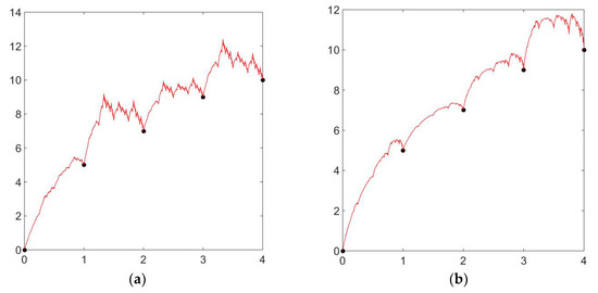
Let $\left(0,0\right),\left(1,5\right),\left(2,7\right),\left(3,9\right),\left(4,10\right)$  be the positive interpolating points, and with these data points, we generate the positive rational cubic fractal interpolation function with different values of shape parameters and scaling factors. Now, for the positive rational cubic fractal interpolation function, we have calculated the shape parameters according to the above theorem. In Figure 3a, we have taken the shape parameter, i.e., $s_j=\left(2,4,4.2,3\right)$  and the scaling factor $\delta =\left(0.15,0.5,0.35,0.47\right)$. The corresponding graph is positive. In Figure 3b and Figure 3c, we used the same shape parameter, i.e.,  $s_j=\left(7,9.8,10.2,11\right)$ but different scaling factors  $\delta =\left(0.24,0.12,0.32,0.55\right)$ and $\delta =\left(0.15,,,0.25,,,0.32,,,0.46\right)$, respectively. We can easily witness the change in shape due to the different vertical scaling factors. In Figure 3d and Figure 3e, we used the same scaling factor, i.e.,  $\delta =\left(0.1,0.12,0.23,0.5\right)$ but different shape parameters, which are $s_j=\left(5,5.8,6.2,7\right)$ and  $s_j=\left(7,9.8,10.2,11\right)$, respectively. The change in the graph of the positive rational cubic fractal interpolation function is due to the different values for signature and shape parameters. Similarly, by taking the shape parameter  $s_j=\left(9,11.2,12.8,13\right)$ and scaling factor,  $\delta =\left(0.15,0.25,0.35,0.45\right)$, Figure 3f is generated, which is another positive graph for the rational cubic fractal interpolation function.

Theorem 11.

Let $\left\{\left(y_m,z_m\right)\in J\times K;m\in M_M\right\}$ be the considered positive dataset, then the zipper-rational cubic fractal interpolation function $S_{\epsilon }^{\delta }$ is positive if the following conditions hold for the shape parameter and scaling factor:

$$0\le {\delta }_j<\min \left\{a_j,{\displaystyle \frac{z_{j+{\epsilon }_j}}{z_1}},{\displaystyle \frac{z_{j+1-{\epsilon }_j}}{z_M}}\right\}$$

$$s_j>\max \left\{0,{\displaystyle \frac{-\left(h_j{d}_{j+{\epsilon }_j}-{\delta }_j\left(y_M-y_1\right)d_1\right)}{z_{j+{\epsilon }_j}-{\delta }_j{z}_1}},{\displaystyle \frac{\left(h_j{d}_{j+1-{\epsilon }_j}-{\delta }_j\left(y_M-y_1\right)d_M\right)}{z_{j+1-{\epsilon }_j}-{\delta }_j{z}_M}},j\in M_{M-1}\right\}$$

Proof. 

To prove that the zipper-rational cubic fractal interpolation function $S_{\epsilon }^{\delta }$ is positive, it will be sufficient to show that $S_{\epsilon }^{\delta }\left(L_j\left(y\right)\right)\ge 0$, and by the hypothesis of the iterated function system, we can say that $S_{\epsilon }^{\delta }\left(L_j\left(y\right)\right)$ will be positive if $u_{j,\epsilon }\left(\theta \right)\ge 0\forall \theta \in \left[0,1\right]$. To prove that $u_{j,\epsilon }\left(\theta \right)\ge 0$ we need to show that $A_{j,\epsilon },B_{j,\epsilon },C_{j,\epsilon }$ and $D_{j,\epsilon }\ge 0$, so we have $A_{j,\epsilon }\ge 0\Rightarrow \left(1+s_j\right)\left(z_{j+{\epsilon }_j}-{\delta }_j{z}_1\right)\ge 0,$ as $s_j$ is a non-negative shape parameter, so

$$\Rightarrow {\delta }_j\le {\displaystyle \frac{z_{j+{\epsilon }_j}}{z_1}}$$

Similarly, $D_{j,\epsilon }\ge 0\Rightarrow z_{j+1-{\epsilon }_j}-{\delta }_j{z}_M\ge 0$, we obtain

$$\Rightarrow {\delta }_j\le {\displaystyle \frac{z_{j+1-{\epsilon }_j}}{z_M}}$$

Now, $B_{j,\epsilon }\ge 0$ if $\left(3+2s_j\right)z_{j+{\epsilon }_j}+\left(1+s_j\right)h_j{d}_{j+{\epsilon }_j}-{\delta }_j\left(\left(3+2s_j\right)z_1+\left(1+s_j\right)\left(y_M-y_1\right)d_1\right)\ge 0$

$$\Rightarrow s_j\ge {\displaystyle \frac{-\left(h_j{d}_{j+{\epsilon }_j}-{\delta }_j\left(y_M-y_1\right)d_1\right)}{z_{j+{\epsilon }_j}-{\delta }_j{z}_1}};j\in M_{M-1}, \mathrm{provided} z_{j+{\epsilon }_j}-{\delta }_j{z}_1>0$$

Similarly, $C_{j,\epsilon }\ge 0$ if $\left(3+s_j\right)z_{j+1-{\epsilon }_j}-h_j{d}_{j+1-{\epsilon }_j}-{\delta }_j\left(\left(3+s_j\right)z_M-\left(y_M-y_1\right)d_M\right)\ge 0$

$$\Rightarrow s_j\ge {\displaystyle \frac{\left(h_j{d}_{j+1-{\epsilon }_j}-{\delta }_j\left(y_M-y_1\right)d_M\right)}{z_{j+1-{\epsilon }_j}-{\delta }_j{z}_M}};j\in M_{M-1}, \mathrm{provided} z_{j+1-{\epsilon }_j}-{\delta }_j{z}_M>0.$$

□

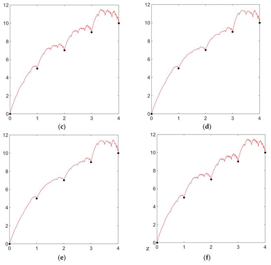
Example 4.

Let $\left(0,0\right),\left(1,5\right),\left(2,7\right),\left(3,9\right),\left(4,10\right)$  be the positive interpolating points, and with these data points, we will be generating the positive zipper-rational cubic fractal interpolation function with different shape parameters, signatures, and scaling factors. In Figure 4a, we used the arbitrary shape parameters, i.e.,  $s_j=\left(2,4,4.2,3\right)$  and the scaling factor and signature are $\delta =\left(0.15,0.5,0.35,0.47\right)$ , and  $\epsilon =\left(1,1,1,1\right)$, respectively. The corresponding graph is non-positive. For the positive zipper-rational cubic fractal interpolation function, we calculated the shape parameters according to the above theorem. In Figure 4b and Figure 4c, we used the same shape parameter, i.e.,  $s_j=\left(7,9.8,10.2,11\right)$ but different scaling factor and signature, i.e., $\delta =\left(0.24,0.12,0.32,0.55\right),$  $\delta =\left(0.15,0.25,0.32,0.46\right)$, and $\epsilon =\left(0,0,0,0\right),$ $\epsilon =\left(1,1,1,1\right)$, respectively. We can clearly witness the change in shape due to the signature and scaling factor. In Figure 4d and Figure 4e, we used the same scaling factor and signature, i.e.,  $\delta =\left(0.1,0.12,0.23,0.5\right),\epsilon =(0,1,0,1)$  but different shape parameters, which are  $s_j=\left(5,5.8,6.2,7\right)$ and $s_j=\left(7,9.8,10.2,11\right)$, respectively. We can witness the change in the graph of the positive zipper-rational cubic fractal interpolation function due to the different values for signature and shape parameters.

If we see Figure 3a and Figure 4a, we have taken the same values for the scaling factor, but for the C¹ rational cubic fractal interpolation function, it is a positive graph. For the C¹ zipper-rational cubic fractal interpolation function, it is a negative graph.

7. Conclusions and Future Work

In this paper, the C¹ rational cubic fractal interpolation function (RCFIF) and C¹ zipper cubic fractal interpolation function (ZRCFIF) with a linear denominator and one shape parameter are constructed. The proposed ZRCFIF becomes the classical rational cubic interpolation function, if we take zero values of both signature and scaling factor. Also, if only the values of the scaling factor are taken to be zero, then ZRCFIF reduces to the classical C¹ zipper-rational cubic interpolation function, and if only the signature is taken to be zero, then it reduces to RCFIF. The uniform convergence of the C¹ rational cubic fractal interpolation function and the C¹ zipper-rational cubic fractal interpolation function to the original function is also discussed. The results are also supported by numerical examples for both the rational cubic fractal interpolation function and the zipper-rational cubic fractal interpolation function. The graphs of the interpolating function are demonstrated for various selections of signature, scaling factor, and shape parameters. If one suitably chooses (as stated in Theorems 10 and 11) the range of scaling factors and shape parameters, then the proposed RQFIF and ZRQFIF preserve positivity.

Figure 1, Figure 2, Figure 3 and Figure 4 demonstrate the sensitivity of the proposed class of fractal interpolation functions with respect to the signature, scaling factors, and shape parameters. We can also see that the zipper fractal interpolation function is more flexible than the fractal interpolation function due to the presence of a signature. Duan et al. [52] demonstrated that cubic spline gives a better approximation with a linear denominator than with quadratic or cubic denominators. In that way, the zipper-rational cubic fractal interpolation function with a linear denominator will give a better approximation as compared to the zipper fractal interpolation function with quadratic or cubic denominators. The proposed C¹ RCFIFs and ZRCFIFs can be used for data visualization and in physics.

For future work, the vertical scaling factor can be replaced by a variable scaling for generating a C¹ rational cubic fractal interpolation function and a C¹ zipper-rational cubic fractal interpolation function with variable scaling.

References

- Schmidt, J.W.; Heß, W. Positivity of cubic polynomials on intervals and positive spline interpolation. BIT Numer. Math. 1988, 28, 340–352. [Google Scholar] [CrossRef]
- Butt, S.; Brodlie, K.W. Preserving positivity using piecewise cubic interpolation. Comput. Graph. 1993, 17, 55–64. [Google Scholar] [CrossRef]
- Sarfraz, M.; Hussain, M.Z. Data visualization using rational spline interpolation. J. Comput. Appl. Math. 2006, 189, 513–525. [Google Scholar] [CrossRef][Green Version]
- Hussain, M.Z.; Sarfraz, M. Positivity-preserving interpolation of positive data by rational cubics. J. Comput. Appl. Math. 2008, 218, 446–458. [Google Scholar] [CrossRef]
- Chernous’ ko, F.L.; Ananievski, I.M.; Reshmin, S.A. Control of Nonlinear Dynamical Systems: Methods and Applications; Springer Science & Business Media: Berlin/Heidelberg, Germany, 2008. [Google Scholar]
- Jayaraman, A.; Belmonte, A. Oscillations of a solid sphere falling through a wormlike micellar fluid. Phys. Rev. E. 2003, 67, 065301. [Google Scholar] [CrossRef]
- Massopust, P. Interpolation and Approximation with Splines and Fractals; Oxford University Press, Inc.: Oxford, UK, 2010. [Google Scholar]
- Barnsley, M.F. Fractals Everywhere; Academic Press: Cambridge, MA, USA, 2014. [Google Scholar]
- Gibert, S.; Massopust, P.R. The exact Hausdorff dimension for a class of fractal functions. J. Math. Anal. Appl. 1992, 168, 171–183. [Google Scholar] [CrossRef]
- Barnsley, M.F. Fractal functions and interpolation. Constr. Approx. 1986, 2, 303–329. [Google Scholar] [CrossRef]
- Hutchinson, J.E. Fractals and self similarity. Indiana Univ. Math. J. 1981, 30, 713–747. [Google Scholar] [CrossRef]
- Barnsley, M.F.; Harrington, A.N. The calculus of fractal interpolation functions. J. Approx. Theory 1989, 57, 14–34. [Google Scholar] [CrossRef]
- Navascués, M.A.; Sebastián, M.V. Smooth fractal interpolation. J. Inequalities Appl. 2006, 2006, 78734. [Google Scholar] [CrossRef]
- Prasad, B.; Katiyar, K.; Singh, B. Trigonometric quadratic fractal interpolation functions. Int. J. Appl. Eng. Res. 2015, 37, 290–302. [Google Scholar]
- Garg, S.; Katiyar, K. A new type of zipper fractal interpolation surfaces and associated bivariate zipper fractal operator. J. Anal. 2023, 31, 3021–3043. [Google Scholar] [CrossRef]
- Gautam, S.S.; Katiyar, K. Alpha fractal rational quintic spline with shape preserving properties. Int. J. Comput. Appl. Math. Comput. Sci. 2023, 3, 113–121. [Google Scholar] [CrossRef]
- Chand, A.K.B.; Vijender, N.; Navascués, M.A. Shape preservation of scientific data through rational fractal splines. Calcolo 2014, 51, 329–362. [Google Scholar] [CrossRef]
- Reddy, K.M.; Chand, A.K.; Viswanathan, P. Data visualization by rational fractal function based on function values. J. Anal. 2020, 28, 261–277. [Google Scholar] [CrossRef]
- Navascués, M.A. Fractal polynomial interpolation. Z. Anal. Ihre Anwendungen 2005, 24, 401–418. [Google Scholar] [CrossRef]
- Banerjee, A.; Akhtar, M.N.; Navascués, M.A. Local α-fractal interpolation function. Eur. Phys. J. Spec. Top. 2023, 232, 1043–1050. [Google Scholar] [CrossRef]
- Feng, Z.; Sun, X. Box-counting dimensions of fractal interpolation surfaces derived from fractal interpolation functions. J. Math. Anal. Appl. 2014, 412, 416–425. [Google Scholar] [CrossRef]
- Akhtar, M.N.; Prasad, M.G.; Navascués, M.A. Box dimensions of α-fractal functions. Fractals 2016, 24, 1650037. [Google Scholar] [CrossRef]
- Nayak, S.R.; Mishra, J.; Palai, G. Analysing roughness of surface through fractal dimension: A review. Image Vis. Comput. 2019, 89, 21–34. [Google Scholar] [CrossRef]
- Ri, S. New types of fractal interpolation surfaces. Chaos Solitons Fractals 2019, 119, 291–307. [Google Scholar] [CrossRef]
- Navascués, M.A.; Akhtar, M.N.; Mohapatra, R. Fractal frames of functions on the rectangle. Fractal Fract. 2021, 5, 42. [Google Scholar] [CrossRef]
- Pandey, M.; Som, T.; Verma, S. Fractal dimension of Katugampola fractional integral of vector-valued functions. Eur. Phys. J. Spec. Top. 2021, 230, 3807–3814. [Google Scholar] [CrossRef]
- Navascués, M.A. Fractal curves on Banach algebras. Fractal Fract. 2022, 6, 722. [Google Scholar] [CrossRef]
- He, C.H.; Liu, C. Fractal dimensions of a porous concrete and its effect on the concrete’s strength. Facta Univ. Ser. Mech. Eng. 2023, 21, 137–150. [Google Scholar] [CrossRef]
- Lal, R.; Selmi, B.; Verma, S. On Dimension of Fractal Functions on Product of the Sierpiński Gaskets and Associated Measures. Results Math. 2024, 79, 73. [Google Scholar] [CrossRef]
- Navascués, M.A. Approximation of fixed points and fractal functions by means of different iterative algorithms. Chaos Solitons Fractals 2024, 180, 114535. [Google Scholar] [CrossRef]
- Chandra, S.; Verma, S.; Abbas, S. Construction of fractal functions using Kannan mappings and smoothness analysis. arXiv 2023, arXiv:2301.03075. [Google Scholar]
- Thangaraj, C.; Easwaramoorthy, D.; Selmi, B.; Chamola, B.P. Generation of fractals via iterated function system of Kannan contractions in controlled metric space. Math. Comput. Simul. 2024, 222, 188–198. [Google Scholar] [CrossRef]
- Garg, S.; Katiyar, K. Positivity and monotonicity shape preserving using rational quintic fractal interpolation functions. Adv. Math. Sci. J. 2020, 9, 5511–5520. [Google Scholar]
- Tyada, K.R.; Chand, A.K.B.; Sajid, M. Shape preserving rational cubic trigonometric fractal interpolation functions. Math. Comput. Simulation. 2021, 90, 866–891. [Google Scholar] [CrossRef]
- Ibraheem, F.; Hussain, M.; Hussain, M.Z.; Bhatti, A.A. Positive data visualization using trigonometric function. J. Appl. Math. 2012, 2012, 247120. [Google Scholar] [CrossRef]
- Dube, M.; Rana, P.S. Positivity preserving interpolation of positive data by rational quadratic trigonometric spline. IOSR J. Math. 2014, 10, 42–47. [Google Scholar] [CrossRef]
- Hussain, M.Z.; Ali, J. Positivity-preserving piecewise rational cubic interpolation. Matematika 2006, 22, 147–153. [Google Scholar]
- Piah, A.R.M.; Unsworth, K. Improved sufficient conditions for monotonic piecewise rational quartic interpolation. Sains Malays. 2011, 40, 1173–1178. [Google Scholar]
- Abbas, M.; Majid, A.A.; Ali, J.M. Monotonicity-preserving C2 rational cubic spline for monotone data. Appl. Math. Comput. 2012, 219, 2885–2895. [Google Scholar] [CrossRef]
- Chand, A.K.B.; Vijender, N. Monotonicity preserving rational quadratic fractal interpolation functions. Adv. Numer. Anal. 2014, 2014, 504825. [Google Scholar] [CrossRef]
- Dube, M.; Tiwari, P. Convexity preserving C2 rational quadratic trigonometric spline. Int. J. Sci. Res. Publ. 2012, 3, 401. [Google Scholar]
- Sharma, S.; Katiyar, K. Preserving convexity through C2 rational quintic fractal interpolation function. InAIP Conf. Proc. 2023, 2735, 040015. [Google Scholar]
- Brodlie, K.W.; Butt, S. Preserving convexity using piecewise cubic interpolation. Comput. Graph. 1991, 15, 15–23. [Google Scholar] [CrossRef]
- Viswanathan, P.; Chand, A.K.B.; Agarwal, R.P. Preserving convexity through rational cubic spline fractal interpolation function. J. Comput. Appl. Math. 2014, 263, 262–276. [Google Scholar] [CrossRef]
- Aseev, V.V.; Tetenov, A.V.; Kravchenko, A.S. On selfsimilar Jordan curves on the plane. Sib. Math. J. 2003, 44, 379–386. [Google Scholar] [CrossRef]
- Aseev, V.V.; Tetenov, A.V. On the self-similar Jordan arcs admitting structure parametrization. Sib. Math. J. 2005, 46, 581–592. [Google Scholar] [CrossRef]
- Jha, S.; Chand, A.K.B. Zipper rational quadratic fractal interpolation functions. In Proceedings of the Fifth International Conference on Mathematics and Computing: ICMC; Springer: Singapore, 2020; pp. 229–241. [Google Scholar]
- Chand, A.K.B. Zipper fractal functions with variable scalings. Adv. Theory Nonlinear Anal. Appl. 2022, 6, 481–501. [Google Scholar]
- Vijay; Chand, A.K.B. Convexity-preserving rational cubic zipper fractal interpolation curves and surfaces. Math. Comput. Appl. 2023, 28, 74. [Google Scholar]
- Chand, A.K.B.; Vijender, N.; Viswanathan, P.; Tetenov, A.V. Affine zipper fractal interpolation functions. BIT Numer. Math. 2020, 60, 319–344. [Google Scholar] [CrossRef]
- Aseev, V.V. On the regularity of self-similar zippers. In Proceedings of the 6-th Russian-Korean International Symposium on Science and Technology, KORUS-2002, Novosibirsk, Russia, 24–30 June 2002; p. 167. [Google Scholar]
- Duan, Q.; Djidjeli, K.; Price, W.G.; Twizell, E.H. The approximation properties of some rational cubic splines. Int. J. Comput. Math. 1999, 72, 155–166. [Google Scholar] [CrossRef]
Disclaimer/Publisher’s Note: The statements, opinions and data contained in all publications are solely those of the individual author(s) and contributor(s) and not of MDPI and/or the editor(s). MDPI and/or the editor(s) disclaim responsibility for any injury to people or property resulting from any ideas, methods, instructions or products referred to in the content. |
© 2024 by the authors. Licensee MDPI, Basel, Switzerland. This article is an open access article distributed under the terms and conditions of the Creative Commons Attribution (CC BY) license (https://creativecommons.org/licenses/by/4.0/).