Abstract
The Hotelling statistic is used to compare the mean vectors of two independent multivariate Gaussian distributions. Nevertheless, this statistic is highly sensitive to outliers and is not suitable for high-dimensional datasets where the number of variables exceeds the sample size. This study introduces a robust permutation test based on the minimum regularized covariance determinant (MRCD) estimator to address these limitations of the two-sample Hotelling statistic. Simulation studies were performed to evaluate the proposed test’s empirical size, power, and robustness. Additionally, the test was applied to both uncontaminated and contaminated Alzheimer’s Disease datasets. The findings from the simulations and real data examples provide clues that the proposed test can be effectively used with high-dimensional data without being impacted by outliers. Finally, an R function within the “MVTests” package was developed to implement the proposed test statistic on real-world data.
Keywords:
robust Hotelling test statistic; high-dimensional data; minimum regularized covariance estimators; permutation test; MVTests MSC:
62G10; 62G35; 62H15; 62P10
1. Introduction
Let and be the distribution of two independent groups. We decide to test the hypothesis given in (1) to see whether the mean parameters of these groups, which have multivariate Gaussian distributions, are equal.
If the scatter parameters of these multivariate distributions are homogeneous and the common covariance matrix is unknown, two samples Hotelling statistics which are given in Equation (2) is used to test the hypothesis defined in (1):
where and are sample sizes of the first and second groups; moreover and are the sample mean vectors of the first and second groups, respectively. Also is the transpose operator. is the pooled covariance matrix and is calculated as below:
where is the sample covariance matrix of the first group and is the sample covariance matrix of the second group. Let be the calculated value of the statistic given in Equation (2). When , we reject the null hypothesis [1,2].
The Hotelling statistic is based on the classical mean vectors and covariance matrices. For this reason, it is heavily sensitive to outliers in the data. The term sensitive means that the estimators are affected by outliers in the data, which means that outliers in the data will cause their estimations to fail. The common solution to this problem is to use robust mean vectors and covariance matrices in the literature. Willems et al. [3] used the minimum covariance determinant (MCD) estimators, Çetin and Aktaş [4] used the minimum volume ellipsoid (MVE) estimators, Mokhtar et al. [5] used the M-estimators for a one-sample Hotelling statistic instead of classical ones. Similarly, Todorov and Filzmoser [6] used the MCD estimators for one-way MANOVA.
Another important problem is that the statistic given in Equation (2) can only be used for low-dimensional datasets, which are . Otherwise, the matrix is singular and the precision matrix cannot be obtained. Therefore, the cannot be calculated. There are many test statistics in the literature to overcome this problem.
Bai and Saranadasa [7] proposed the statistic in Equation (4). Because there is no precision matrix in the test statistics given in Equation (4), this statistic can be used in high-dimensional data. We can perform this statistic on any real data via the apval_Bai1996() function in the R package called “highmean” [8].
where is a trace operator.
Srivastava and Du [9] suggested using a diagonal matrix instead of a covariance matrix. The diagonal elements of this diagonal matrix are variances in matrix . Therefore, Srivastava and Du [9] proposed a test statistic that can be used in high-dimensional data by removing the covariance information. This statistic is given in Equation (5). The p-value for this statistic can be obtained by using the apval_Sri2008() function in the R package called “highmean” [8].
where is a diagonal matrix, and is the diagonal element of matrix . Moreover, is the correlation matrix, and .
Chen and Qin [10] suggested the test statistic given in Equation (6). The p-value for the statistic can be obtained by using the apval_Chen2010() function in the R package called “highmean” [8].
These test statistics lose power when the vector contains many zero elements [11,12]. For this reason, Cai, Liu and Xia [11] proposed a supremum test statistic. The p-value for this supremum statistic can be calculated by using the apval_Cai2014() function in the R package called “highmean” [8].
The test statistics ( given in Equations (4)–(7) can be used to test the hypothesis in (2) with high-dimensional data. However, these test statistics are still sensitive to outliers because they are based on classical estimators.
As mentioned before, Willems, Pison, Rousseeuw and Van Aelst [3] and Todorov and Filzmoser [6] used the MCD estimators to obtain robust tests. However, it is well known that the MCD estimators can only be used for low-dimensional data. To overcome this lack of MCD estimators, Boudt et al. [13] developed the minimum regularized covariance determinant (MRCD) estimators. MRCD estimators can be obtained robustly in high-dimensional data, unlike MCD ones. Detailed information about MRCD estimators is given in Section 2. Bulut [14] used the MRCD estimators to propose a robust Hoteling statistic for one sample.
The main purpose of this study is to propose a test that can be used in high-dimensional data and is not sensitive to outliers in the data. For this aim, we extend the approach developed by Bulut (2023b) to two-sample cases. Moreover, we aim to use our test procedure on real data by generating R functions in the “MVTests” package [15].
The remainder of the study is designed as follows. In Section 2, the MRCD estimators are introduced. Section 3 defines the proposed robust Hotelling statistic and test procedure. In Section 4, a robust version of proposed by Cai, Liu and Xia [11] is introduced. We perform a simulation study to compare the performance of our test procedure and alternative tests in Section 5. In Section 6, we perform tests on real example data to compare the performance of the tests. We introduce the R functions, which can be used to perform our test statistic in Section 7. Finally, we provide conclusions in Section 8.
2. Minimum Regularized Covariance Determinant (MRCD) Estimators
Willems, Pison, Rousseeuw and Van Aelst [3] and Todorov and Filzmoser [6] used the MCD estimators to obtain robust test statistics. However, these estimators cannot be used when .
Boudt, Rousseeuw, Vanduffel and Verdonck [13] proposed Minimum Regularized Covariance Determinant (MRCD) estimators of location and scatter parameters without affecting outliers in high-dimensional data. The MRCD estimator has good breakdown point properties of the MCD estimator [13,14].
To calculate MRCD estimations, firstly, we standardize data by using the median and as the univariate location and scatter estimators [16]; then, we use the target matrix. This matrix is symmetric and positive definite. The regularized covariance matrix of any subset , which is obtained from standardized data, is calculated as below:
where is the regularization parameter, is the consistency factor defined by Croux and Haesbroeck [17], and
MRCD estimations are obtained from the subset which is obtained by solving the minimization problem given in Equation (10).
where is the set, which consists of all subsets with size in data. Finally, the MRCD location and scatter estimators are obtained as given in Equations (11) and (12).
where and are eigenvalues and eigenvectors matrices of , respectively. Also, is calculated as below:
More detailed information about MRCD estimators is available in [13]. In this study, we used the “rrcov” package in the R software for calculations regarding the MRCD estimators [18]. While we use the package, we assume that we know the outlier rate of the data. Moreover, we prefer to use the default values of the regularization parameter (rho) and target matrix. The function automatically calculates these values from the dataset.
3. Proposed Hotelling Test
The Hotelling statistic, which is used to compare mean vectors of two independent groups, is given in Equation (2). As mentioned before, however, this statistic cannot be used in high-dimensional data and is sensitive to outliers in data. In this study, we propose a test statistic that can be used in high-dimensional data without being affected by outliers in data. This statistic is given in Equation (14).
where and are the sample size of the first and second groups, respectively. and are MRCD estimations of location parameters of the first and second groups, respectively. The matrix C is a robust pooled covariance matrix and it is calculated as in Equation (15):
where and are the MRCD covariance matrices of the first and second samples, respectively.
Because the finite-sample distribution of MRCD estimators is unknown, Bulut [14] used an approach distribution for a one-sample case. This approach is used by Willems, Pison, Rousseeuw and Van Aelst [3] and Todorov and Filzmoser [6] in low-dimensional data. However, we prefer a permutation test instead of any asymptotic distribution because the asymptotic distribution approach needs too much calculation time. As a result, we propose the robust permutation test to compare the mean vectors of two independent groups in high-dimensional data as below:
- Calculate the MRCD estimations of the first and second groups.
- Calculate the value based on Equation (14). Let be this calculated value.
- Compound all observations as one sample with size .
- Under the null hypothesis, randomly separate observations such that observations are in the first group and observations are in the second group.
- Calculate the value based on Equation (14) for the generated synthetic groups.
- Repeat steps (iii–v) N times. Here, N is the permutation number.
- Calculate the p-value as given in Equation (16):
According to the test algorithm, we can calculate the p-value directly without any distribution assumption. Moreover, we can calculate this p-value in high-dimensional data. We reject the null hypothesis when the p-value is less than the significance level. This test procedure can be performed on any real example data with the R function introduced in Section 7.
Like other permutation tests, the performance of the proposed test statistics is based on the permutation number, and once the permutation number increases, the results will be more stable.
4. Robust CLX Test
Wang et al. [19] proposed a robust alternative to the test procedure suggested by Cai, Liu and Xia [11]. We show this test statistic for consistence. is defined in Equation (17):
where , and is the common precision matrix for trimmed mean vectors and . and are the trimmed mean vectors for the first and second groups, respectively.
Let a random sample be and is the order statistic of this sample. For the trimming level , we can calculate the trimmed mean of this sample given by:
Therefore, the trimmed mean vector can be obtained by calculating all the trimmed means of the p-variables for each group. According to this, we can define the trimmed mean vectors for the first and second groups as and , respectively.
As a result, we can reject the null hypothesis when . Here, is the th quantile of the Gumbel distribution. More detailed information about the test statistic is available from Wang, Lin and Tang [19].
5. Simulation Study
In this section, we design a simulation study to compare , and , which is our proposed test regarding the empirical size, power and robustness properties. We test the null hypothesis in all simulation designs, and we take in all cases. Here, is a zero vector.
We randomly sample observations from the multivariate Gaussian distributions for the first group and for the second group. The common and homogeneity covariance matrix of these distributions is generated based on three different models used by Cai, Liu and Xia [11] as below:
- Model 1: , where
- Model 2: , where for .
- Model 3: , and , where , , , , , otherwise.
For all the simulation studies, we use sample size values , and variable numbers . Therefore, we study high-dimensional data in all cases.
5.1. Empirical Size (Type-1) of Tests
In this subsection, we perform a simulation study to compare the empirical size performance of , , and . We generate random samples from the multivariate Gaussian distributions and , respectively. We set such that the null hypothesis is true in all cases. We obtain based on Models 1–3. We test the null hypothesis with , , and for each sample, and we calculate the empirical size of all the tests as the ratio of rejecting the true null hypothesis. We reject the null hypothesis when . The results are given in Table 1.

Table 1.
Empirical sizes of test statistics.
Table 1 compares the empirical sizes of the test statistics. We can see that the empirical sizes of are reasonably close to the nominal level of 5%. As the sample size increases, the empirical sizes of become close to the nominal value, while the empirical sizes of go away from the nominal value. We can see in Table 1 that the and statistics have similar empirical size values.
5.2. Power of Tests
We perform a simulation study to compare the powers of , , and in this subsection. We generate random samples from the multivariate Gaussian distributions and , respectively. We set such that the null hypothesis is false in all cases. In all cases, . We define with two different approaches as below:
- Fixed magnitude: , for with the equal probability, and .
- Varied magnitude: , is generated from for , and .
Here, we use two different m values of and . Also, denotes the minimum integer which is greater than . We obtain based on Models 1–3. We test the null hypothesis with , , and for each sample. Then, we calculate the power of all the tests as the ratio of rejecting the false null hypothesis. We reject the null hypothesis when . The results are given in Table 2. According to Table 2, the power loss of the is acceptable because the datasets generated are not contaminated.
Table 2.
Power of test statistics.
5.3. Robustness of Tests
In this subsection, we perform a simulation study to investigate the robustness performance of , , and . We generate 90% of random samples from the multivariate Gaussian distributions and , respectively. Moreover, we generate the remaining 10% of samples from the multivariate Gaussian distributions and , respectively. Here, and . We obtain based on Models 1–3. Therefore, we contaminate samples with a 10% outlier ratio.
We draw a plot to show the effect of outliers in Figure 1. We generate 27 random observations from the first population and 27 observations from the second population such that . Moreover, we generate three random observations for the first group from the population , and three observations for the second group from the population . is generated based on Model-1 in each case in Figure 1. Also, and . We used the multidimensional scaling method to reduce the dimension from 25 to 2.
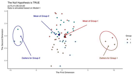
Figure 1.
Scatter plots for instance outliers problem in high-dimensional data.
According to Figure 1, we can see that the outliers in the two groups move the equal mean vectors away from each other. For this reason, a non-robust test may reject the null hypothesis, which is true in real data, while a robust test must fail to reject the null hypothesis without being affected by outliers. In this section, we compare the robustness performance of each test.
We test the null hypothesis with , , and for each sample, and we reject the null hypothesis when . Before the datasets are contaminated, the null hypothesis is true. If any test statistic is robust to outliers in data, it must reject the null hypothesis with a percentage close to the nominal significance level (5%). For this reason, we calculate the robustness performance as the ratio of rejecting the true null hypothesis. The results are given in Table 3.
Table 3.
Robustness of test statistics.
According to Table 3, it is abundantly clear that the statistic is robust to outliers, while other statistics are heavily sensitive to outliers. The statistic has similar performance with contaminated data and uncontaminated data but this performance is unacceptable because the empirical size values are lower than the nominal value of 5%.
6. Real Example
Alzheimer’s disease (AD) is a cognitive impairment disorder marked by memory loss and a decline in functional abilities beyond what is typical for a given age, making it the most prevalent cause of dementia in the elderly. Biologically, Alzheimer’s disease is linked to amyloid-β (Aβ) brain plaques and brain tangles associated with a form of the Tau protein [20].
While medical imaging can be useful in predicting the onset of the disease, there is also a growing interest in potential cost-effective fluid biomarkers that can be extracted from plasma or cerebrospinal fluid (CSF). Currently, there are several acknowledged non-imaging biomarkers, including protein levels of specific forms of the Aβ and Tau proteins and the Apolipoprotein E genotype. The Apolipoprotein E genotype has three primary variants: E2, E3, and E4, with the E4 allele most closely associated with AD [21,22].
In a clinical study conducted by Craig-Schapiro et al. [23] involving 333 patients, including those with mild but well-characterized cognitive impairment and healthy individuals, CSF samples were collected from all subjects. The study aimed to determine if individuals in the early stages of impairment could be distinguished from cognitively healthy individuals. They included in the analysis demographic attributes like age and gender, the Apolipoprotein E genotype, protein measurements of Aβ, Tau, and a phosphorylated version of Tau (referred to as pTau), protein measurements of 124 exploratory biomarkers, and clinical dementia scores [20]. This data is available with the name AlzheimerDisease in the “AppliedPredictiveModeling” package in R software [24].
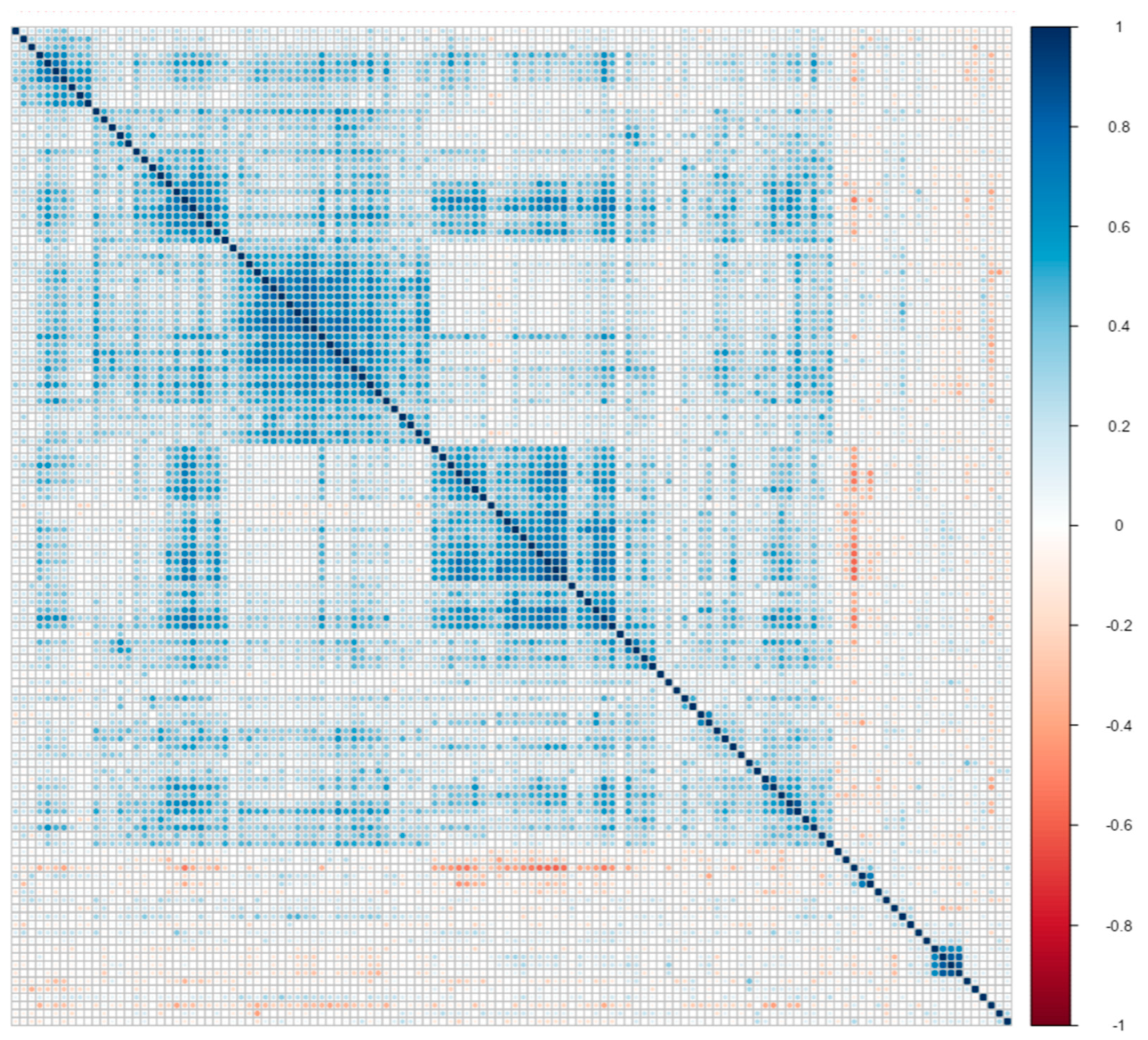
In this subsection, we use only 124 protein measurements as biomarkers of AD. Therefore, we have variables in our data. Moreover, we use a subset that contains 106 high-risk patients with Apolipoprotein E genotype E3E4, as Wang, Lin and Tang [19] do. subjects of them are “impaired”, and subjects of them are “healthy”. Then, we standardized all variables. As a result, we have high-dimensional data, and we provide a correlation plot of this data in Figure 2.

Figure 2.
Correlation plot matrix . Columns and rows were sorted with clustering methods.
We aim to compare the mean vectors of two groups (“impaired” vs. “healthy”). For this purpose, firstly, we assume that our data does not contain outliers, and so we test the null hypothesis with , , and . The results of the tests are given in the “Clean Data” part of Table 4. According to this part, all the tests reject the null hypothesis.
Table 4.
Test results of Alzheimer’s Disease data.
After analysis of the clean data, we contaminate 10% of the data such that the difference between the mean vectors decreases. For this aim, we determine the last four observations in Impaired group-1 and the last six observations in Healthy group-2 such that the mean values of all the variables in group-1 are equal to 2, and the mean values of all the variables in group-2 are equal to 1.8. Therefore, the difference between the mean vectors of the groups is 0.2 for all variables. Despite the mean vectors of uncontaminated data in each group initially differing, the introduction of outliers has mitigated this disparity. For this reason, the appropriate decision for any test is to reject the null hypothesis without being affected by outliers we added into the groups.
We test these contaminated data again to compare the mean vectors with , , and . The results of the tests are given in the “Contaminated Data” part of Table 4. According to Table 4, still rejects the null hypothesis without being affected by outliers, whereas the other tests fail to reject the null hypothesis and are affected by outliers. These results show that is a robust test statistic to compare two mean vectors in high-dimensional datasets, while the other test statistics are not robust enough for this purpose.
7. Software Availability
We construct a function RperT2() to perform the proposed robust permutational test on real datasets in the R package called “MVTests” [15]. In this function, the data matrix of the first group must be entered into X1, and the data matrix of the second group must be entered into X2. The alpha argument determines the trimming ratio and must take a value from interval 0–1 (default; alpha = 0.75). The N argument determines the iteration number (default; N = 100). We give an example in Appendix A to demonstrate how to use this function to perform the proposed test on data in R.
8. Conclusions
In multivariate inference, the two-sample Hotelling statistic is popular. However, this statistic cannot be used for contaminated or high-dimensional data.
There are many studies in the literature that demonstrate that Hotelling statistics are not sensitive to outliers. The common approach in these studies is to use robust location and scatter estimation instead of classical ones [4,5,6]. However, these statistics cannot be used in high-dimensional data.
On the other hand, there are also many studies that obtain statistics, which can be used in high-dimensional data in the literature [9,10,11,12]. However, these statistics are sensitive to outliers in data.
Wang, Lin and Tang [19] proposed a robust test statistic that can be used in high-dimensional data. However, their statistic is useful for cell-wise contaminated data.
In this study, we propose a robust test statistic for high-dimensional data. This statistic is based on MRCD estimations. Because the finite-sample distribution of MRCD estimators is unknown, we propose using a permutation test without needing any asymptotic distribution.
We perform simulation studies to compare the empirical size, power and robustness performances of , , and in clean and row-wise contaminated data. According to the simulation studies, the empirical sizes of are close to the nominal level (5%), the powers of are acceptable, and is not sensitive to outliers in data.
We perform tests on clean and contaminated Alzheimer’s Disease data. In the clean case, all tests reject the null hypothesis. In the contaminated case, however, only rejects the null hypothesis, unlike other statistics.
Finally, we construct the RperT2() function to perform our proposed test on real data in the R package entitled MVTests [15]. We believe that our proposed statistic is a valuable contribution to multivariate inference for high-dimensional data.
In high-dimensional datasets, the missing values problem is another problem similar to the outlier one. Future studies will focus on how the proposed test statistic can cope with this problem in the case of missing observations in high-dimensional data.
Author Contributions
Conceptualization, H.B.; methodology, H.B.; software, H.B.; validation, S.I., N.F. and O.A.; formal analysis, H.B.; investigation, H.B. and N.F.; resources, S.I.; data curation, O.A.; writing—original draft preparation, H.B. and S.I.; writing—review and editing, H.B., N.F. and O.A.; visualization, H.B.; supervision, H.B.; funding acquisition, N.F. and O.A. All authors have read and agreed to the published version of the manuscript.
Funding
This research received no external funding.
Data Availability Statement
We used synthetic datasets for simulations and Alzheimer’s Disease datasets for real examples in this study. The Alzheimer’s Disease data is available with the name AlzheimerDisease in the “AppliedPredictiveModeling” package in R software [24].
Acknowledgments
The authors thank the editors and four referees for their helpful, constructive comments, which have helped improve the quality and presentation of the paper.
Conflicts of Interest
The authors declare no conflicts of interest.
Appendix A
RperT2() function in the MVTests package [15] performs the proposed test on real high-dimensional data. The general usage of the function is as below:
RperT2 (X1, X2, alpha = 0.75, N = 100)
Here, X1 and X2 is the data matrix for the first and second groups, respectively. Also, they must be matrix or data.frame. alpha is numeric parameter controlling the size of the subsets over which the determinant is minimized. The allowed values are between 0.5 and 1 and the default is 0.75. Finally, N is the permutation number and its default value is 100.
To give an example, firstly, we generate random high dimensional data in R as below:
> x<-mvtnorm::rmvnorm (n = 10, sigma = diag(20), mean = rep(0,20))
> y<-mvtnorm::rmvnorm (n = 10, sigma = diag(20), mean = rep(1,20))
To generate random data from multivariate normal distribution, we use the rmvnorm() function in the package mvtnorm in R. It is seen that both samples have 10 observations and 20 variables. Therefore, we can say the data is high-dimensional. Moreover, we can see the mean vector of first group is and the mean vector of second group is . The covariance matrices of both groups are the same as the identity matrix. As a result, we expect to find a statistically significant difference between group means.
We can perform the proposed test on this data with default alpha and N values as below:
| > install.packages(“MVTests”) |
| > library(MVTests) |
| > RperT2(X1 = x, X2 = y) |
| $T2 |
| TR2 |
| 419.7017 |
| $p.value |
| [1] 0 |
Function returns us and the p-value. Because the p-value is < 0.001, we reject the null hypothesis with a 99.9% confidence level.
Finally, we can perform the proposed test on this data with different alpha and N values as below:
| > install.packages(“MVTests”) |
| > library(MVTests) |
| > RperT2(X1 = x, X2 = y, alpha = 0.9, N = 300)) |
| $T2 |
| TR2 |
| 378.2798 |
| $p.value |
| [1] 0 |
Function returns us and the p-value. Because the p-value is <0.001, we reject the null hypothesis with a 99.9% confidence level.
References
- Rencher, A.C. Methods of Multivariate Analysis; John Willey & Sons, Inc.: Montreal, QC, Canada, 2002. [Google Scholar]
- Bulut, H. Multivariate Statistical Methods with R Applications, 2nd ed.; Nobel Academic Publishing: Ankara, Turkey, 2023. [Google Scholar]
- Willems, G.; Pison, G.; Rousseeuw, P.J.; Van Aelst, S. A Robust Hotelling Test. Metrika 2002, 55, 125–138. [Google Scholar] [CrossRef]
- Cetin, M.; Altunay, S.A. Hotelling’s T2 Statistic Based on Minimum-Volume-Ellipsoid Estimator. Gazi Univ. J. Sci. 2003, 16, 691–695. [Google Scholar]
- Mokhtar, M.A.A.M.; Yusoff, N.S.; Liang, C.Z. Robust Hotelling’s T2 Statistic Based on M-Estimator. J. Phys. Conf. Ser. 2021, 1988, 012116. [Google Scholar] [CrossRef]
- Todorov, V.; Filzmoser, P. Robust Statistic for the One-Way Manova. Comput. Stat. Data Anal. 2010, 54, 37–48. [Google Scholar] [CrossRef]
- Bai, Z.; Saranadasa, H. Effect of High Dimension: By an Example of a Two Sample Problem. Stat. Sin. 1996, 6, 311–329. [Google Scholar]
- Lin, L.; Pan, W. Highmean: Two-Sample Tests for High-Dimensional Mean Vectors; R Package Version 3.0; 2016. Available online: https://cran.r-project.org/web/packages/highmean/index.html (accessed on 23 August 2024).
- Srivastava, M.S.; Du, M. A Test for the Mean Vector with Fewer Observations than the Dimension. J. Multivar. Anal. 2008, 99, 386–402. [Google Scholar] [CrossRef]
- Chen, S.X.; Qin, Y.-L. A Two-Sample Test for High-Dimensional Data with Applications to Gene-Set Testing. Ann. Stat. 2010, 38, 808–835. [Google Scholar] [CrossRef]
- Cai, T.T.; Liu, W.D.; Xia, Y. Two-Sample Test of High Dimensional Means under Dependence. J. R. Stat. Soc. Ser. B Stat. Methodol. 2014, 76, 349–372. [Google Scholar]
- Xu, G.; Lin, L.; Wei, P.; Pan, W. An Adaptive Two-Sample Test for High-Dimensional Means. Biometrika 2016, 103, 609–624. [Google Scholar] [CrossRef] [PubMed]
- Boudt, K.; Rousseeuw, P.J.; Vanduffel, S.; Verdonck, T. The Minimum Regularized Covariance Determinant Estimator. Stat. Comput. 2020, 30, 113–128. [Google Scholar] [CrossRef]
- Bulut, H. A Robust Hotelling Test Statistic for One Sample Case in High Dimensional Data. Commun. Stat.-Theory Methods 2023, 52, 4590–4604. [Google Scholar] [CrossRef]
- Bulut, H. An R Package for Multivariate Hypothesis Tests: Mvtests. Technol. Appl. Sci. 2019, 14, 132–138. [Google Scholar] [CrossRef]
- Rousseeuw, P.J.; Croux, C. Alternatives to the Median Absolute Deviation. J. Am. Stat. Assoc. 1993, 88, 1273–1283. [Google Scholar] [CrossRef]
- Croux, C.; Haesbroeck, G. Influence Function and Efficiency of the Minimum Covariance Determinant Scatter Matrix Estimator. J. Multivar. Anal. 1999, 71, 161–190. [Google Scholar] [CrossRef]
- Todorov, V.; Filzmoser, P. An Object-Oriented Framework for Robust Multivariate Analysis. J. Stat. Softw. 2010, 32, 1–47. [Google Scholar] [CrossRef]
- Wang, W.; Lin, N.; Tang, X. Robust Two-Sample Test of High-Dimensional Mean Vectors under Dependence. J. Multivar. Anal. 2019, 169, 312–329. [Google Scholar] [CrossRef]
- Kuhn, M.; Johnson, K. Applied Predictive Modeling; Springer: New York, NY, USA, 2013; Volume 26. [Google Scholar]
- Kim, J.; Basak, J.M.; Holtzman, D.M. The Role of Apolipoprotein E in Alzheimer’s Disease. Neuron 2009, 63, 287–303. [Google Scholar] [CrossRef] [PubMed]
- Bu, G. Apolipoprotein E and Its Receptors in Alzheimer’s Disease: Pathways, Pathogenesis and Therapy. Nat. Rev. Neurosci. 2009, 10, 333–344. [Google Scholar] [CrossRef] [PubMed]
- Craig-Schapiro, R.; Kuhn, M.; Xiong, C.; Pickering, E.H.; Liu, J.; Misko, T.P.; Perrin, R.J.; Bales, K.R.; Soares, H.; Fagan, A.M.; et al. Multiplexed Immunoassay Panel Identifies Novel Csf Biomarkers for Alzheimer’s Disease Diagnosis and Prognosis. PLoS ONE 2011, 6, e18850. [Google Scholar] [CrossRef] [PubMed]
- Kuhn, M.; Johnson, K. Appliedpredictivemodeling: Functions and Data Sets for ‘Applied Predictive Modeling’; R Package Version 1. 2018. Available online: https://cran.r-project.org/web/packages/AppliedPredictiveModeling/index.html (accessed on 23 August 2024).
Disclaimer/Publisher’s Note: The statements, opinions and data contained in all publications are solely those of the individual author(s) and contributor(s) and not of MDPI and/or the editor(s). MDPI and/or the editor(s) disclaim responsibility for any injury to people or property resulting from any ideas, methods, instructions or products referred to in the content. |
© 2024 by the authors. Licensee MDPI, Basel, Switzerland. This article is an open access article distributed under the terms and conditions of the Creative Commons Attribution (CC BY) license (https://creativecommons.org/licenses/by/4.0/).