A Complete Characterization of Linear Dependence and Independence for All 4-by-4 Metric Matrices

Abstract

In this article, we study the properties of 4-by-4 metric matrices and characterize their dependence and independence by ${\mathcal{M}}^{4\times 4}=({\mathcal{M}}^{4\times 4}-D{\mathcal{M}}^{4\times 4})\cup D{\mathcal{M}}^{4\times 4}$, where $D{\mathcal{M}}^{4\times 4}$ is the set of all dependent metric matrices. $D{\mathcal{M}}^{4\times 4}$ is further characterized by $D{\mathcal{M}}^{4\times 4}=D{\mathcal{M}}_1^{4\times 4}\cup D{\mathcal{M}}_2^{4\times 4}$, where $D{\mathcal{M}}_2^{4\times 4}$ is characterized by $D{\mathcal{M}}_2^{4\times 4}=D{\mathcal{M}}_{21}^{4\times 4}\cup D{\mathcal{M}}_{22}^{4\times 4}$. These characterizations provide some insightful findings that go beyond the Euclidean distance or Euclidean distance matrix and link the distance functions to vector spaces, which offers some theoretical and application-related advantages. In the application parts, we show that the metric matrices associated with all Minkowski distance functions over four different points are linearly independent, and that the metric matrices associated with any four concyclic points are also linearly independent.

1. Introduction

Distance functions, or metrics, are always a fascinating topic in research due to their diverse and intuitive applications [1,2]. In this article, we investigate the relationship between linear dependence and metrics. For each metric d with a finite domain size, say n, it can be represented (or the nodes relabeled) by $n!$ metric matrices (or ${\left\{M_d^j\right\}}_{j=1}^{n!}$). Because the simultaneous exchange of any two rows and the exchange of any two columns does not change the value of the determinants, i.e., $|M_d^j|=|M_d^k|$ for all $1\le i,j\le n!$, it is sufficient to study one representation. Here, ${\mathbb{R}}_{+}^{4\times 4}$ denotes the set of all 4-by-4 real matrices where the diagonal elements are 0 and the off-diagonal elements are all positive real numbers.

Definition 1.

${\mathcal{M}}^{4\times 4}=\left\{\left[\begin{array}{cccc}0& d_{12}& d_{13}& d_{14}\\ d_{12}& 0& d_{23}& d_{24}\\ d_{13}& d_{23}& 0& d_{34}\\ d_{14}& d_{24}& d_{34}& 0\end{array}\right]\in {\mathbb{R}}_{+}^{4\times 4}:|d_{ij}-d_{jk}|\le d_{ik}\le d_{ij}+d_{jk},\right.1\le i,j,k\le 4\}.$

Officially, we should probably call these matrices ‘distance matrices’. However, in order not to confuse them with the typical Eulidean Distance Matrix (or EDM) [3,4] based on square distances, we simply call our simple distance-based matrices metric matrices. In this paper, we study and characterize the necessary and sufficient conditions for the dependence and independence of ${\mathcal{M}}^{4\times 4}$. First, we provide the necessary conditions for the linear dependence of a metric matrix. These conditions are mainly found in Lemma 1. Then, we show that any metric matrix containing at least one real triangular triplet would not satisfy the necessary conditions, as shown in Claims 1 and 3. This leads directly to the further characterization of the necessary condition, as shown in Claims 2 and 4 and summarized in Lemma 2 and 3. We then show the sufficient conditions for linear dependence by constructing three sets of disjoint dependence metric matrices: $D{\mathcal{M}}_1^{4\times 4},D{\mathcal{M}}_{21}^{4\times 4}$, and $D{\mathcal{M}}_{22}^{4\times 4}$, respectively defined in Definitions 2, 4, and 5. We show that these categorized metric matrices fully characterize the dependent metric matrices in ${\mathcal{M}}^{4\times 4}$ via Theorem 1, Corollary 1, and Lemma 4. The entire theorems, associated presentations, and derivations are presented in Section 2. Applications of these theorems are presented in Section 3 and Section 4.

2. Theories and Derivations

Lemma 1

(Necessary conditions). If $\mathcal{D}\in {\mathcal{M}}^{4\times 4}$ and $\left|\mathcal{D}\right|=0$, then

$$d_{12}={\displaystyle \frac{d_{13}{d}_{24}+d_{14}{d}_{23}\pm 2\sqrt{d_{13}{d}_{14}{d}_{23}{d}_{24}}}{d_{34}}},$$

or

$$d_{12}{d}_{34}={[\sqrt{d_{13}{d}_{24}}\pm \sqrt{d_{14}{d}_{23}}]}^2.$$

Proof. 

Let $\mathcal{D}=\left[\begin{array}{cc}{D}_{11}& D_{12}\\ D_{21}& D_{22}\end{array}\right]$, where $D_{11}=\left[\begin{array}{cc}0& d_{12}\\ d_{12}& 0\end{array}\right];$ $D_{12}=\left[\begin{array}{cc}{d}_{13}& d_{14}\\ d_{23}& d_{24}\end{array}\right];$ $D_{21}=\left[\begin{array}{cc}{d}_{13}& d_{23}\\ d_{14}& d_{24}\end{array}\right];$ $D_{22}=\left[\begin{array}{cc}0& d_{34}\\ d_{34}& 0\end{array}\right].$ □

Because $D_{22}$ is invertible (thus, $\left|\mathcal{D}\right|=|D_{22}|\times |D_{11}-D_{12}{D}_{22}^{-1}{D}_{21}|$), we have $|D_{11}-D_{12}{D}_{22}^{-1}{D}_{21}|=0$, i.e.,

$$\left|\left[\begin{array}{cc}0& d_{12}\\ d_{12}& 0\end{array}\right]-\left[\begin{array}{cc}{\displaystyle \frac{2d_{13}{d}_{14}}{d_{34}}}& {\displaystyle \frac{d_{13}{d}_{24}+d_{14}{d}_{23}}{d_{34}}}\\ {\displaystyle \frac{d_{13}{d}_{24}+d_{14}{d}_{23}}{d_{34}}}& {\displaystyle \frac{2d_{23}{d}_{24}}{d_{34}}}\end{array}\right]\right|=0,$$

i.e.,

$$d_{12}^2-\left({\displaystyle \frac{2t}{d_{34}}}\right)d_{12}+[{\displaystyle \frac{t^2}{d_{34}^2}}-{\displaystyle \frac{4d_{13}{d}_{14}{d}_{23}{d}_{24}}{d_{34}^2}}]=0,$$

where $t=d_{13}{d}_{24}+d_{14}{d}_{23}$. Therefore,

$$d_{12}={\displaystyle \frac{t\pm 2\sqrt{d_{13}{d}_{14}{d}_{23}{d}_{24}}}{d_{34}}}.$$

Claim 1.

If

$$\left\{\begin{array}{c}{d}_{12}{⊛}_1(d_{13}+d_{23})\hfill \\ d_{12}{⊛}_2(d_{14}+d_{24})\hfill \\ d_{34}{⊛}_3(d_{13}+d_{14})\hfill \\ d_{34}{⊛}_4(d_{23}+d_{24})\hfill \end{array}\right.,$$

where ${⊛}_i\in \{<,=\}$ for all $1\le i\le 4$ and $\left|\right\{i\in \{1,2,3,4\}:{⊛}_i{\equiv }^{\prime }{=}^{\prime }\left\}\right|\le 3$, then $d_{12}\ne {\displaystyle \frac{d_{13}{d}_{24}+d_{14}{d}_{23}+2\sqrt{d_{13}{d}_{14}{d}_{23}{d}_{24}}}{d_{34}}}$.

Proof. 

Assume $d_{12}={\displaystyle \frac{d_{13}{d}_{24}+d_{14}{d}_{23}+2\sqrt{d_{13}{d}_{14}{d}_{23}{d}_{24}}}{d_{34}}}$. From the premise, we have $d_{12}{d}_{34}{⊛}_{13}(d_{13}+d_{23})(d_{13}+d_{14})$; $d_{12}{d}_{34}{⊛}_{14}(d_{13}+d_{23})(d_{23}+d_{24})$; $d_{12}{d}_{34}{⊛}_{23}(d_{14}+d_{24})(d_{13}+d_{14})$; $d_{12}{d}_{34}{⊛}_{24}(d_{14}+d_{24})(d_{23}+d_{24})$, where ${⊛}_{ij}{\equiv }^{\prime }{=}^{\prime }$ if ${⊛}_i{\equiv }^{\prime }{=}^{\prime }$ and ${⊛}_j{\equiv }^{\prime }{=}^{\prime }$, otherwise ${⊛}_{ij}{\equiv }^{\prime }{<}^{\prime }$. These results lead to

$$\begin{array}{cc}\hfill [d_{13}{d}_{24}+2\sqrt{d_{13}{d}_{14}{d}_{23}{d}_{24}}]{⊛}_{13}[d_{13}^2+d_{13}{d}_{14}+d_{13}{d}_{23}],& \end{array}$$

(1)

$$\begin{array}{cc}\hfill [d_{14}{d}_{23}+2\sqrt{d_{13}{d}_{14}{d}_{23}{d}_{24}}]{⊛}_{14}[d_{23}^2+d_{13}{d}_{23}+d_{23}{d}_{24}],& \end{array}$$

(2)

$$\begin{array}{cc}\hfill [d_{14}{d}_{23}+2\sqrt{d_{13}{d}_{14}{d}_{23}{d}_{24}}]{⊛}_{23}[d_{14}^2+d_{13}{d}_{14}+d_{14}{d}_{24}],& \end{array}$$

(3)

$$\begin{array}{c}\hfill [d_{13}{d}_{24}+2\sqrt{d_{13}{d}_{14}{d}_{23}{d}_{24}}]{⊛}_{24}[d_{24}^2+d_{14}{d}_{24}+d_{23}{d}_{24}].\end{array}$$

(4)

Now, we can divide both sides of Equations (1)–(4) by $d_{13},d_{23},d_{14}$, and $d_{24}$, respectively, yielding

$$\begin{array}{cc}\hfill [d_{24}+2\sqrt{{\displaystyle \frac{d_{14}{d}_{23}{d}_{24}}{d_{13}}}}]{⊛}_{13}[d_{13}+d_{14}+d_{23}],& \end{array}$$

(5)

$$\begin{array}{cc}\hfill [d_{14}+2\sqrt{{\displaystyle \frac{d_{13}{d}_{14}{d}_{24}}{d_{23}}}}]{⊛}_{14}[d_{23}+d_{13}+d_{24}],& \end{array}$$

(6)

$$\begin{array}{cc}\hfill [d_{23}+2\sqrt{{\displaystyle \frac{d_{13}{d}_{23}{d}_{24}}{d_{14}}}}]{⊛}_{23}[d_{14}+d_{13}+d_{24}],& \end{array}$$

(7)

$$\begin{array}{c}\hfill [d_{13}+2\sqrt{{\displaystyle \frac{d_{13}{d}_{14}{d}_{23}}{d_{24}}}}]{⊛}_{24}[d_{24}+d_{14}+d_{23}].\end{array}$$

(8)

Multiplying Equation (5) by $d_{14}$ and (6) by $d_{24}$ yields

$$\begin{array}{cc}\hfill \left(d_{14}{d}_{24}\right){⊛}_{13}[d_{13}{d}_{14}+d_{14}^2+d_{14}{d}_{23}-2d_{14}\sqrt{{\displaystyle \frac{d_{14}{d}_{23}{d}_{24}}{d_{13}}}}],& \end{array}$$

(9)

$$\begin{array}{c}\hfill \left(d_{14}{d}_{24}\right){⊛}_{14}[d_{23}{d}_{24}+d_{13}{d}_{24}+d_{24}^2-2d_{24}\sqrt{{\displaystyle \frac{d_{13}{d}_{14}{d}_{24}}{d_{23}}}}].\end{array}$$

(10)

Substituting Equations (9) and (10) into (3) and (4), respectively, yields

$$\begin{array}{c}\hfill 2\sqrt{d_{13}{d}_{14}{d}_{23}{d}_{24}}+2d_{14}\sqrt{{\displaystyle \frac{d_{14}{d}_{23}{d}_{24}}{d_{13}}}}{⊛}_{123}2(d_{13}{d}_{14}+d_{14}^2),\\ \hfill 2\sqrt{d_{13}{d}_{14}{d}_{23}{d}_{24}}+2d_{24}\sqrt{{\displaystyle \frac{d_{13}{d}_{14}{d}_{24}}{d_{23}}}}{⊛}_{124}2(d_{23}{d}_{24}+d_{24}^2),\end{array}$$

where ${⊛}_{123}{\equiv }^{\prime }{=}^{\prime }$ if ${⊛}_1\equiv {⊛}_2\equiv {⊛}_3{\equiv }^{\prime }{=}^{\prime }$ and ${⊛}_{123}{\equiv }^{\prime }{<}^{\prime }$ otherwise, and where ${⊛}_{124}{\equiv }^{\prime }{=}^{\prime }$ if ${⊛}_1\equiv {⊛}_2\equiv {⊛}_4{\equiv }^{\prime }{=}^{\prime }$ and ${⊛}_{124}{\equiv }^{\prime }{<}^{\prime }$ otherwise. Furthermore, the equations can be simplified as follows:

$$\begin{array}{c}\hfill \sqrt{{\displaystyle \frac{d_{23}{d}_{24}}{d_{13}{d}_{14}}}}[d_{13}{d}_{14}+d_{14}^2]{⊛}_{123}[d_{13}{d}_{14}+d_{14}^2],\\ \hfill \sqrt{{\displaystyle \frac{d_{13}{d}_{14}}{d_{23}{d}_{24}}}}[d_{23}{d}_{24}+d_{24}^2]{⊛}_{124}[d_{23}{d}_{24}+d_{24}^2],\end{array}$$

i.e., $\left(d_{13}{d}_{14}\right){⊛}_{124}\left(d_{23}{d}_{24}\right){⊛}_{123}\left(d_{13}{d}_{14}\right)$, i.e., $\left(d_{13}{d}_{14}\right)<\left(d_{13}{d}_{14}\right)$, as $\left|\right\{i\in \{1,2,3,4\}:{⊛}_i{\equiv }^{\prime }{=}^{\prime }\left\}\right|\le 3$. This yields a contradiction; hence, $d_{12}\ne {\displaystyle \frac{d_{13}{d}_{24}+d_{14}{d}_{23}+2\sqrt{d_{13}{d}_{14}{d}_{23}{d}_{24}}}{d_{34}}}$. □

Remark 1.

In order to save space for our expositions, this claim and the following claims, lemmas, theorems, etc., are not expressed in the traditional way. In principle, to capture the conditions for the premises of the triangle inequlaity, we need $2^4=16$ batches of premises. Instead, we use the notation ⊛ together with

$$\left|\right\{i\in \{1,2,3,4\}:{⊛}_i{\equiv }^{\prime }{=}^{\prime }\left\}\right|\le 3,$$

to denote all remaining cases (except the premise with the equations based on triangle equality: $d_{12}=d_{13}+d_{23};d_{12}=d_{14}+d_{24};d_{34}=d_{13}+d_{14};d_{34}=d_{23}+d_{24}$). In other words, this claim or the following similar statements deal with uniform triangle equality cases. Strictly speaking, if we adopt the traditional representation we would have fifteen claims for this claim alone; thus, we use the notation ⊛ to save space. Another advantage of our presentation is it keeps the derivations as concise as possible and makes it easier for readers to check the validity of the statements.

Claim 2.

If $d_{12}={\displaystyle \frac{d_{13}{d}_{24}+d_{14}{d}_{23}+2\sqrt{d_{13}{d}_{14}{d}_{23}{d}_{24}}}{d_{34}}}$, then $d_{13}=d_{24}$ and $d_{23}=d_{14}$.

Proof. 

Per Claim 1, if we have $d_{12}={\displaystyle \frac{d_{13}{d}_{24}+d_{14}{d}_{23}+2\sqrt{d_{13}{d}_{14}{d}_{23}{d}_{24}}}{d_{34}}}$, then

$$\left\{\begin{array}{c}{d}_{12}=d_{13}+d_{23}\hfill \\ d_{12}=d_{14}+d_{24}\hfill \\ d_{34}=d_{13}+d_{14}\hfill \\ d_{34}=d_{23}+d_{24}\hfill \end{array}\right.,$$

i.e., $d_{13}+d_{23}=d_{14}+d_{24}$ and $d_{13}+d_{14}=d_{23}+d_{24}$, i.e., $d_{13}=d_{24}$ and $d_{23}=d_{14}$. □

Lemma 2.

$d_{12}={\displaystyle \frac{d_{13}{d}_{24}+d_{14}{d}_{23}+2\sqrt{d_{13}{d}_{14}{d}_{23}{d}_{24}}}{d_{34}}}$ iff $d_{13}=d_{24}$; $d_{23}=d_{14}$; $d_{12}=d_{34}=d_{13}+d_{23}$.

Proof. 

Per Claim 2, $d_{13}=d_{24}$ and $d_{23}=d_{14}$, i.e., $d_{12}{d}_{34}=d_{13}{d}_{24}+d_{14}{d}_{23}+2\sqrt{d_{13}{d}_{14}{d}_{23}{d}_{24}}={[d_{13}+d_{14}]}^2$. Because $d_{34}\le d_{13}+d_{14}$, it follows that $d_{12}\ge d_{13}+d_{14}=d_{24}+d_{14}$. From the property $d_{12}\le d_{14}+d_{24}$, we have $d_{12}=d_{13}+d_{14}=d_{34}$. On the other hand, if $d_{13}=d_{24}$; $d_{23}=d_{14}$; $d_{12}=d_{34}=d_{13}+d_{23}$, then ${\displaystyle \frac{d_{13}{d}_{24}+d_{14}{d}_{23}+2\sqrt{d_{13}{d}_{14}{d}_{23}{d}_{24}}}{d_{34}}}={\displaystyle \frac{{(d_{13}+d_{23})}^2}{d_{34}}}=d_{34}=d_{12}$. □

Claim 3.

If

$$\left\{\begin{array}{c}|d_{13}-d_{23}|{⊚}_1{d}_{12}\hfill \\ |d_{14}-d_{24}|{⊚}_2{d}_{12}\hfill \\ |d_{13}-d_{14}|{⊚}_3{d}_{34}\hfill \\ |d_{23}-d_{24}|{⊚}_4{d}_{34}\hfill \end{array}\right.,$$

where ${⊚}_i\in \{<,=\}$ for all $1\le i\le 4$, and $\left|\right\{i\in \{1,2,3,4\}:{⊚}_i{\equiv }^{\prime }{=}^{\prime }\left\}\right|\le 3$, then $d_{12}\ne {\displaystyle \frac{d_{13}{d}_{24}+d_{14}{d}_{23}-2\sqrt{d_{13}{d}_{14}{d}_{23}{d}_{24}}}{d_{34}}}$.

Proof. 

Assume $d_{12}={\displaystyle \frac{d_{13}{d}_{24}+d_{14}{d}_{23}-2\sqrt{d_{13}{d}_{14}{d}_{23}{d}_{24}}}{d_{34}}}$. From the premise, we have $(d_{13}-d_{23})(d_{13}-d_{14}){⊚}_{13}{d}_{12}{d}_{34}$; $(d_{23}-d_{13})(d_{23}-d_{24}){⊚}_{14}{d}_{12}{d}_{34}$; $(d_{14}-d_{24})(d_{14}-d_{13}){⊚}_{23}{d}_{12}{d}_{34}$; $(d_{14}-d_{24})(d_{23}-d_{24}){⊚}_{24}{d}_{12}{d}_{34}$, where ${⊚}_{ij}{\equiv }^{\prime }{=}^{\prime }$ if ${⊚}_i{\equiv }^{\prime }{=}^{\prime }$ and ${⊚}_j{\equiv }^{\prime }{=}^{\prime }$, otherwise ${⊚}_{ij}{\equiv }^{\prime }{<}^{\prime }$. These results lead to

$$\begin{array}{cc}\hfill [d_{13}^2-d_{13}{d}_{14}-d_{13}{d}_{23}]{⊚}_{13}[d_{13}{d}_{24}-2\sqrt{d_{13}{d}_{14}{d}_{23}{d}_{24}}],& \end{array}$$

(11)

$$\begin{array}{cc}\hfill [d_{23}^2-d_{13}{d}_{23}-d_{23}{d}_{24}]{⊚}_{14}[d_{14}{d}_{23}-2\sqrt{d_{13}{d}_{14}{d}_{23}{d}_{24}}],& \end{array}$$

(12)

$$\begin{array}{cc}\hfill [d_{14}^2-d_{13}{d}_{14}-d_{14}{d}_{24}]{⊚}_{23}[d_{14}{d}_{23}-2\sqrt{d_{13}{d}_{14}{d}_{23}{d}_{24}}],& \end{array}$$

(13)

$$\begin{array}{c}\hfill [d_{24}^2-d_{14}{d}_{24}-d_{23}{d}_{24}]{⊚}_{24}[d_{13}{d}_{24}-2\sqrt{d_{13}{d}_{14}{d}_{23}{d}_{24}}].\end{array}$$

(14)

In fact, the notation ${⊚}_{ij}$ is meant to represent the equation ${\alpha }_1{\alpha }_2={\beta }_1{\beta }_2$ if and only if ${\alpha }_1={\beta }_1$ and ${\alpha }_2={\beta }_2$. Now, we can divide both sides of Equations (11)–(14) by $d_{13},d_{23},d_{14}$ and $d_{24}$, respectively, to yield

$$\begin{array}{cc}\hfill [d_{13}-d_{14}-d_{23}]{⊚}_{13}[d_{24}-2\sqrt{{\displaystyle \frac{d_{14}{d}_{23}{d}_{24}}{d_{13}}}}],& \end{array}$$

(15)

$$\begin{array}{cc}\hfill [d_{23}-d_{13}-d_{24}]{⊚}_{14}[d_{14}-2\sqrt{{\displaystyle \frac{d_{13}{d}_{14}{d}_{24}}{d_{23}}}}],& \end{array}$$

(16)

$$\begin{array}{cc}\hfill [d_{14}-d_{13}-d_{24}]{⊚}_{23}[d_{23}-2\sqrt{{\displaystyle \frac{d_{13}{d}_{23}{d}_{24}}{d_{14}}}}],& \end{array}$$

(17)

$$\begin{array}{c}\hfill [d_{24}-d_{14}-d_{23}]{⊚}_{24}[d_{13}-2\sqrt{{\displaystyle \frac{d_{13}{d}_{14}{d}_{23}}{d_{24}}}}].\end{array}$$

(18)

Multiplying Equation (15) by $d_{14}$ and (16) by $d_{24}$ yields

$$\begin{array}{cc}\hfill \left(d_{13}{d}_{14}\right){⊚}_{13}[d_{14}{d}_{24}+d_{14}^2+d_{14}{d}_{23}-2d_{14}\sqrt{{\displaystyle \frac{d_{14}{d}_{23}{d}_{24}}{d_{13}}}}],& \end{array}$$

(19)

$$\begin{array}{c}\hfill \left(d_{23}{d}_{24}\right){⊚}_{14}[d_{14}{d}_{24}+d_{13}{d}_{24}+d_{24}^2-2d_{24}\sqrt{{\displaystyle \frac{d_{13}{d}_{14}{d}_{24}}{d_{23}}}}].\end{array}$$

(20)

Substituting Equations (19) and (20) into (13) and (14), respectively, yields

$$\begin{array}{c}\hfill 2\sqrt{d_{13}{d}_{14}{d}_{23}{d}_{24}}+2d_{14}\sqrt{{\displaystyle \frac{d_{14}{d}_{23}{d}_{24}}{d_{13}}}}{⊚}_{123}2(d_{14}{d}_{23}+d_{14}{d}_{24}),\\ \hfill 2\sqrt{d_{13}{d}_{14}{d}_{23}{d}_{24}}+2d_{24}\sqrt{{\displaystyle \frac{d_{14}{d}_{13}{d}_{24}}{d_{23}}}}{⊚}_{124}2(d_{13}{d}_{24}+d_{14}{d}_{24}),\end{array}$$

where ${⊚}_{123}{\equiv }^{\prime }{=}^{\prime }$ if ${⊚}_1\equiv {⊚}_2\equiv {⊚}_3{\equiv }^{\prime }{=}^{\prime }$, otherwise ${⊚}_{123}{\equiv }^{\prime }{<}^{\prime }$ and where ${⊚}_{124}{\equiv }^{\prime }{=}^{\prime }$ if ${⊚}_1\equiv {⊚}_2\equiv {⊚}_4{\equiv }^{\prime }{=}^{\prime }$, otherwise ${⊚}_{124}{\equiv }^{\prime }{<}^{\prime }$. Furthermore, the equations can be simplified as follows:

$$\begin{array}{c}\hfill \sqrt{d_{13}{d}_{14}{d}_{23}{d}_{24}}[1+{\displaystyle \frac{d_{14}}{d_{13}}}]{⊚}_{123}{d}_{14}[d_{23}+d_{24}],\\ \hfill \sqrt{d_{13}{d}_{14}{d}_{23}{d}_{24}}[1+{\displaystyle \frac{d_{24}}{d_{23}}}]{⊚}_{124}{d}_{24}[d_{13}+d_{14}],\end{array}$$

i.e.,

$$\begin{array}{c}\hfill \sqrt{d_{13}{d}_{14}{d}_{23}{d}_{24}}{⊚}_{123}{\displaystyle \frac{d_{13}{d}_{14}(d_{23}+d_{24})}{d_{13}+d_{14}}},\end{array}$$

(21)

$$\begin{array}{c}\hfill \sqrt{d_{13}{d}_{14}{d}_{23}{d}_{24}}{⊚}_{124}{\displaystyle \frac{d_{23}{d}_{24}(d_{13}+d_{14})}{d_{23}+d_{24}}}.\end{array}$$

(22)

Multiplying Equation (21) with (22) together yields $d_{13}{d}_{14}{d}_{23}{d}_{24}{⊚}_{1234}{d}_{13}{d}_{14}{d}_{23}{d}_{24}$, where ${⊚}_{1234}{\equiv }^{\prime }{=}^{\prime }$ if ${⊚}_1\equiv {⊚}_2\equiv {⊚}_3\equiv {⊚}_4{\equiv }^{\prime }{=}^{\prime }$ and ${⊚}_{1234}{\equiv }^{\prime }{<}^{\prime }$ otherwise. In fact, the notation ${⊚}_{ijk}$ is meant to represent the equation ${\alpha }_1{\alpha }_2{\alpha }_3={\beta }_1{\beta }_2{\beta }_2$ if and only if ${\alpha }_1={\beta }_1$ and ${\alpha }_2={\beta }_2$ and ${\alpha }_3={\beta }_3$. Hence, $d_{13}{d}_{14}{d}_{23}{d}_{24}<d_{13}{d}_{14}{d}_{23}{d}_{24}$, as $\left|\right\{i\in \{1,2,3,4\}:{⊚}_i{\equiv }^{\prime }{=}^{\prime }\left\}\right|\le 3$. This yields a contradiction; hence, $d_{12}\ne {\displaystyle \frac{d_{13}{d}_{24}+d_{14}{d}_{23}-2\sqrt{d_{13}{d}_{14}{d}_{23}{d}_{24}}}{d_{34}}}$. □

Claim 4.

If $d_{12}={\displaystyle \frac{d_{13}{d}_{24}+d_{14}{d}_{23}-2\sqrt{d_{13}{d}_{14}{d}_{23}{d}_{24}}}{d_{34}}}$, then

$$\left\{\begin{array}{c}{d}_{12}=|d_{13}-d_{23}|\hfill \\ d_{12}=|d_{14}-d_{24}|\hfill \\ d_{34}=|d_{13}-d_{14}|\hfill \\ d_{34}=|d_{23}-d_{24}|\hfill \end{array}\right..$$

Proof. 

This follows immediately from Claim 3. □

Lemma 3.

$d_{12}={\displaystyle \frac{d_{13}{d}_{24}+d_{14}{d}_{23}-2\sqrt{d_{13}{d}_{14}{d}_{23}{d}_{24}}}{d_{34}}}$ iff $d_{13}=d_{24}$; $d_{23}=d_{14}$; $d_{12}=d_{34}=|d_{13}-d_{14}|$.

Proof. 

Without loss of generality, per Claim 4, let us assume $d_{13}>d_{14}$ and $d_{23}>d_{24}$; then, we can identify Equations (15) and (18) with

$$\begin{array}{cc}\hfill [d_{13}-d_{14}-d_{23}]=[d_{24}-2\sqrt{{\displaystyle \frac{d_{14}{d}_{23}{d}_{24}}{d_{13}}}}],& \end{array}$$

(23)

$$\begin{array}{cc}\hfill [d_{23}-d_{13}-d_{24}]=[d_{14}-2\sqrt{{\displaystyle \frac{d_{13}{d}_{14}{d}_{24}}{d_{23}}}}],& \end{array}$$

(24)

$$\begin{array}{cc}\hfill [d_{14}-d_{13}-d_{24}]=[d_{23}-2\sqrt{{\displaystyle \frac{d_{13}{d}_{23}{d}_{24}}{d_{14}}}}],& \end{array}$$

(25)

$$\begin{array}{c}\hfill [d_{24}-d_{14}-d_{23}]=[d_{13}-2\sqrt{{\displaystyle \frac{d_{13}{d}_{14}{d}_{23}}{d_{24}}}}].\end{array}$$

(26)

Subtracting Equation (24) from (23) yields

$$\begin{array}{c}\hfill d_{13}-d_{23}=\sqrt{{\displaystyle \frac{d_{14}{d}_{24}}{d_{13}{d}_{23}}}}[d_{13}-d_{23}].\end{array}$$

(27)

Then, we argue $d_{13}\ne d_{23}$; if $d_{13}=d_{23}$, then per Claim 4 we have $d_{34}=d_{13}-d_{14}=d_{23}-d_{24}$. Thusm $d_{14}=d_{24}$, i.e., $d_{12}=0$, which is not possible. Hence, $d_{13}\ne d_{23}$; thus, per Equation (27), ${\displaystyle \frac{d_{14}{d}_{24}}{d_{13}{d}_{23}}}=1$, i.e.,

$$\begin{array}{c}\hfill d_{14}{d}_{24}=d_{13}{d}_{23}.\end{array}$$

(28)

Substituting Equation (28) into either Equation (23), (24), (25), or (26), we have

$$\begin{array}{c}\hfill d_{13}+d_{23}=d_{14}+d_{24}=q.\end{array}$$

(29)

From Equations (28) and (29), we have $d_{14}(q-d_{14})=d_{13}(q-d_{13})$, i.e., $q=d_{13}+d_{14}$, i.e., $d_{14}=d_{23}$ and $d_{13}=d_{24}$. Thus, from the premise, $d_{12}{d}_{34}={[d_{13}-d_{14}]}^2$. Per Claim 4, we know that $d_{34}=|d_{13}-d_{14}|$; hence, we have $d_{12}=d_{34}=|d_{13}-d_{34}|$. □

Based on the above-mentioned theorems, claims, etc., we can identify the dependence metric matrices as follows.

Definition 2.

(First-type dependence metric matrices)

$D{\mathcal{M}}_1^{4\times 4}:=\left\{\left[\begin{array}{cccc}0& \alpha +\gamma & \gamma & \alpha \\ \alpha +\gamma & 0& \alpha & \gamma \\ \gamma & \alpha & 0& \alpha +\gamma \\ \alpha & \gamma & \alpha +\gamma & 0\end{array}\right]:\alpha ,\gamma \in {\mathbb{R}}_{+}\right\}.$

Definition 3.

(Second-type dependence metric matrices)

$D{\mathcal{M}}_2^{4\times 4}:=\left\{\left[\begin{array}{cccc}0& |\alpha -\gamma |& \gamma & \alpha \\ |\alpha -\gamma |& 0& \alpha & \gamma \\ \gamma & \alpha & 0& |\alpha -\gamma |\\ \alpha & \gamma & |\alpha -\gamma |& 0\end{array}\right]:\alpha ,\gamma \in {\mathbb{R}}_{+},\alpha \ne \gamma \right\}$.

Definition 4.

(First subtype of second-type dependence metric matrices)

$D{\mathcal{M}}_{21}^{4\times 4}:=\left\{\left[\begin{array}{cccc}0& \gamma -\alpha & \gamma & \alpha \\ \gamma -\alpha & 0& \alpha & \gamma \\ \gamma & \alpha & 0& \gamma -\alpha \\ \alpha & \gamma & \gamma -\alpha & 0\end{array}\right]:\alpha ,\gamma \in {\mathbb{R}}_{+},\gamma >\alpha \right\}$.

Definition 5.

(Second subtype of second-type dependence metric matrices)

$D{\mathcal{M}}_{22}^{4\times 4}:=\left\{\left[\begin{array}{cccc}0& \alpha -\gamma & \gamma & \alpha \\ \alpha -\gamma & 0& \alpha & \gamma \\ \gamma & \alpha & 0& \alpha -\gamma \\ \alpha & \gamma & \alpha -\gamma & 0\end{array}\right]:\alpha ,\gamma \in {\mathbb{R}}_{+},\alpha >\gamma \right\}$.

Definition 6.

$D{\mathcal{M}}^{4\times 4}=D{\mathcal{M}}_1^{4\times 4}\cup D{\mathcal{M}}_2^{4\times 4}$.

Observing that $D{\mathcal{M}}_{21}^{4\times 4}\cup D{\mathcal{M}}_{22}^{4\times 4}=D{\mathcal{M}}_2^{4\times 4}$ and $D{\mathcal{M}}_1^{4\times 4}\cap D{\mathcal{M}}_2^{4\times 4}=D{\mathcal{M}}_{21}^{4\times 4}\cap D{\mathcal{M}}_{22}^{4\times 4}=\varnothing$. We show that these definitions are sufficient to characterize the set of dependence and independence metric matrices.

Theorem 1.

$D{\mathcal{M}}^{4\times 4}\subseteq {\mathcal{M}}^{4\times 4}$ is the maximal set of all the linearly dependent 4-by-4 metric matrices.

Proof. 

The result follows immediately from Lemmas 1–3. □

Corollary 1.

${\mathcal{M}}^{4\times 4}-D{\mathcal{M}}^{4\times 4}$ is the maximal set of all the linearly independent 4-by-4 metric matrices.

Theorem 2.

For all pairs $(a,b)\in {\mathbb{R}}^2$ with $ab\ge 0$ and $a+b>0$:

1. 

$D{\mathcal{M}}_1^{4\times 4}$ is closed under positive linear combinations, i.e., if $K,H\in D{\mathcal{M}}_1^{4\times 4}$, then $aK+bH\in D{\mathcal{M}}_1^{4\times 4}$.

2. 

$D{\mathcal{M}}_{21}^{4\times 4}$ is closed under positive linear combinations.

3. 

$D{\mathcal{M}}_{22}^{4\times 4}$ is closed under positive linear combinations.

Proof. 

The first statement is trivial. Here, we prove the second and third statements. Let $K=[k_{ij}],H=[h_{ij}]\in D{\mathcal{M}}_{21}^{4\times 4}$, let $(a,b)$ be an arbitrary pair such that $ab\ge 0$ and $a+b>0$, and let $C=[c_{ij}]=aK+bH$; then,

$$\begin{array}{cc}\hfill c_{13}=a{k}_{13}+b{h}_{13}=a{k}_{24}+b{h}_{24}=c_{24}& \\ \hfill c_{14}=a{k}_{14}+b{h}_{14}=a{k}_{23}+b{h}_{23}=c_{23}& \\ \hfill c_{12}=a{k}_{12}+b{h}_{12}=a(k_{13}-k_{23})+b(h_{13}-h_{23})& \\ \hfill =(a{k}_{13}+b{h}_{13})-(a_{23}+b_{23})=c_{13}-c_{23};\end{array}$$

furthermore,

$$\begin{array}{cc}\hfill c_{12}=c_{13}-c_{23}=c_{24}-c_{14}=c_{21}& \\ \hfill c_{34}=a{k}_{34}+b{h}_{34}=a{k}_{12}+b{h}_{12}=c_{12}.\end{array}$$

Hence, we have shown that $aK+bH\in D{\mathcal{M}}_{21}^{4\times 4}$. A similar proof applies to the third statement. □

Example 1.

If $\mathcal{D}=\left[\begin{array}{cccc}0& 8& 3& 5\\ 8& 0& 5& 3\\ 3& 5& 0& 8\\ 5& 3& 8& 0\end{array}\right]$, $\mathcal{E}=\left[\begin{array}{cccc}0& 2& 5& 3\\ 2& 0& 3& 5\\ 5& 3& 0& 2\\ 3& 5& 2& 0\end{array}\right]$, and $\mathcal{F}=\left[\begin{array}{cccc}0& 2& 3& 5\\ 2& 0& 5& 3\\ 3& 5& 0& 2\\ 5& 3& 2& 0\end{array}\right]$, then $\mathcal{D}\in D{\mathcal{M}}_1^{4\times 4}\subseteq {\mathcal{M}}^{4\times 4},\mathcal{E}\in D{\mathcal{M}}_{21}^{4\times 4}\subseteq {\mathcal{M}}^{4\times 4},\mathcal{F}\in D{\mathcal{M}}_{22}^{4\times 4}\subseteq {\mathcal{M}}^{4\times 4}$, and $\left|\mathcal{D}\right|=\left|\mathcal{E}\right|=\left|\mathcal{F}\right|=0$.

The completely characterization of the above relation can be seen in Figure 1:

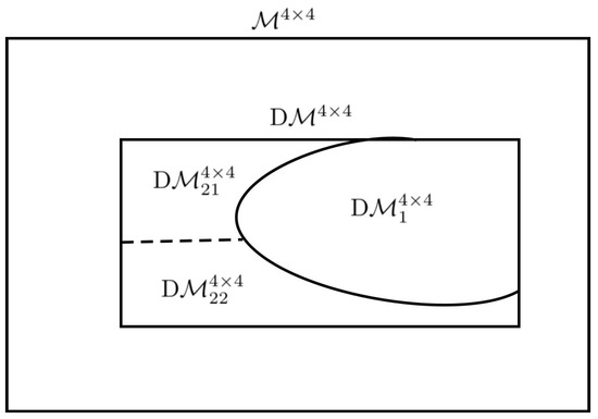
Figure 1. Characterization of dependence and independence: ${\mathcal{M}}^{4\times 4}-D{\mathcal{M}}^{4\times 4}$ is the set of all the linearly independent metric matrices in which $D{\mathcal{M}}^{4\times 4}$ consists of two parts, $D{\mathcal{M}}_1^{4\times 4}$ and $D{\mathcal{M}}_2^{4\times 4}$; moreover, $D{\mathcal{M}}_2^{4\times 4}$ is divided into $D{\mathcal{M}}_{21}^{4\times 4}$ and $D{\mathcal{M}}_{22}^{4\times 4}$.

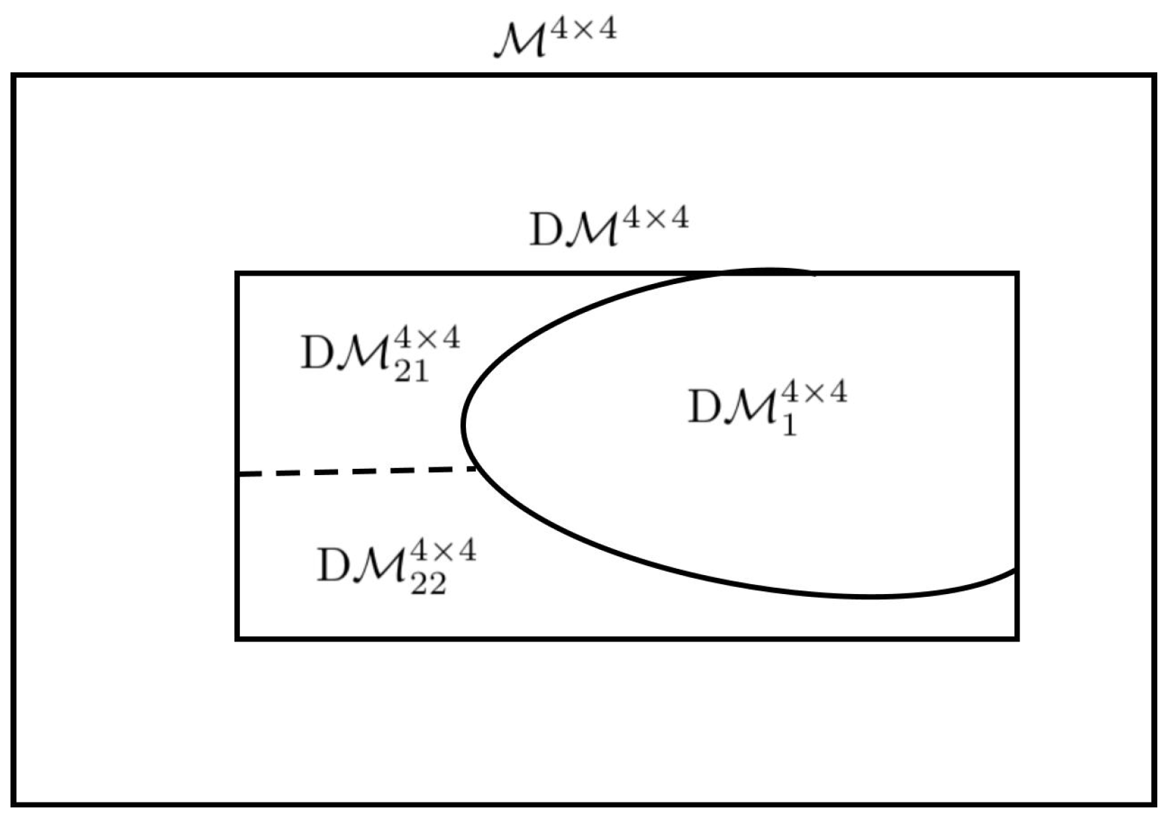
Let $K\in {\mathcal{M}}^{4\times 4}$ be arbitrary, and let $K_{i\leftrightarrow j}\in {\mathcal{M}}^{4\times 4}$ denote the metric matrix after swapping the i-th and j-th rows and the i-th and j-th columns of K.

Claim 5.

1. 

If $K\in D{\mathcal{M}}_1^{4\times 4}$, then $K_{1\leftrightarrow 2},K_{3\leftrightarrow 4}\in D{\mathcal{M}}_1^{4\times 4}$; $K_{2\leftrightarrow 3},K_{1\leftrightarrow 4}\in D{\mathcal{M}}_{21}^{4\times 4}$; $K_{1\leftrightarrow 3},K_{2\leftrightarrow 4}\in D{\mathcal{M}}_{22}^{4\times 4}$.

2. 

If $K\in D{\mathcal{M}}_{21}^{4\times 4}$, then $K_{1\leftrightarrow 3},K_{2\leftrightarrow 4}\in D{\mathcal{M}}_{21}^{4\times 4}$; $K_{1\leftrightarrow 4},K_{2\leftrightarrow 3}\in D{\mathcal{M}}_1^{4\times 4}$; $K_{1\leftrightarrow 2},K_{3\leftrightarrow 4}\in D{\mathcal{M}}_{22}^{4\times 4}$;

3. 

If $K\in D{\mathcal{M}}_{22}^{4\times 4}$, then $K_{1\leftrightarrow 4},K_{2\leftrightarrow 3}\in D{\mathcal{M}}_{22}^{4\times 4}$; $K_{1\leftrightarrow 3},K_{2\leftrightarrow 4}\in D{\mathcal{M}}_1^{4\times 4}$; $K_{1\leftrightarrow 2},K_{3\leftrightarrow 4}\in D{\mathcal{M}}_{21}^{4\times 4}$.

Proof. 

Let $K=\left[\begin{array}{cccc}0& \alpha +\gamma & \gamma & \alpha \\ \alpha +\gamma & 0& \alpha & \gamma \\ \gamma & \alpha & 0& \alpha +\gamma \\ \alpha & \gamma & \alpha +\gamma & 0\end{array}\right]\in D{\mathcal{M}}_1^{4\times 4}$ be arbitrary. Then, $K_{1\leftrightarrow 2},K_{3\leftrightarrow 4}$ only swap $\alpha$ and $\gamma$ in K, i.e., $K_{1\leftrightarrow 2},K_{3\leftrightarrow 4}\in D{\mathcal{M}}_1^{4\times 4}$. Furthermore, $K_{2\leftrightarrow 3}=\left[\begin{array}{cccc}0& \gamma & \alpha +\gamma & \alpha \\ \gamma & 0& \alpha & \alpha +\gamma \\ \alpha +\gamma & \alpha & 0& \gamma \\ \alpha & \alpha +\gamma & \gamma & 0\end{array}\right]\in D{\mathcal{M}}_{21}^{4\times 4}$ and $K_{2\leftrightarrow 4}=\left[\begin{array}{cccc}0& \alpha & \gamma & \alpha +\gamma \\ \alpha & 0& \alpha +\gamma & \gamma \\ \gamma & \alpha +\gamma & 0& \alpha \\ \alpha +\gamma & \gamma & \alpha & 0\end{array}\right]\in D{\mathcal{M}}_{22}^{4\times 4}$. Similarly, $K_{1\leftrightarrow 4}\in D{\mathcal{M}}_{21}^{4\times 4}$ and $K_{1\leftrightarrow 3}\in D{\mathcal{M}}_{22}^{4\times 4}$. Now, let $K=\left[\begin{array}{cccc}0& \gamma -\alpha & \gamma & \alpha \\ \gamma -\alpha & 0& \alpha & \gamma \\ \gamma & \alpha & 0& \gamma -\alpha \\ \alpha & \gamma & \gamma -\alpha & 0\end{array}\right]\in D{\mathcal{M}}_{21}^{4\times 4}$ be arbitrary, where $\gamma >\alpha$. Then, $K_{2\leftrightarrow 3}=\left[\begin{array}{cccc}0& \gamma & \gamma -\alpha & \alpha \\ \gamma & 0& \alpha & \gamma -\alpha \\ \gamma -\alpha & \alpha & 0& \gamma \\ \alpha & \gamma -\alpha & \gamma & 0\end{array}\right]\in D{\mathcal{M}}_1^{4\times 4}$ and $K_{2\leftrightarrow 4}=\left[\begin{array}{cccc}0& \gamma & \gamma -\alpha & \alpha \\ \gamma & 0& \alpha & \gamma -\alpha \\ \gamma -\alpha & \alpha & 0& \gamma \\ \alpha & \gamma -\alpha & \gamma & 0\end{array}\right]\in D{\mathcal{M}}_{21}^{4\times 4}$; similarly, $K_{1\leftrightarrow 3}\in D{\mathcal{M}}_{21}^{4\times 4},K_{1\leftrightarrow 4}\in D{\mathcal{M}}_1^{4\times 4}$, and $K_{1\leftrightarrow 2},K_{3\leftrightarrow 4}\in D{\mathcal{M}}_{22}^{4\times 4}$. Lastly, let $K=\left[\begin{array}{cccc}0& \alpha -\gamma & \gamma & \alpha \\ \alpha -\gamma & 0& \alpha & \gamma \\ \gamma & \alpha & 0& \alpha -\gamma \\ \alpha & \gamma & \alpha -\gamma & 0\end{array}\right]\in D{\mathcal{M}}_{22}^{4\times 4}$ be arbitrary, where $\gamma <\alpha$; then, $K_{1\leftrightarrow 2}=\left[\begin{array}{cccc}0& \alpha -\gamma & \alpha & \gamma \\ \alpha -\gamma & 0& \gamma & \alpha \\ \alpha & \gamma & 0& \alpha -\gamma \\ \gamma & \alpha & \alpha -\gamma & 0\end{array}\right]\in D{\mathcal{M}}_{21}^{4\times 4}$, as does $K_{3\leftrightarrow 4}\in D{\mathcal{M}}_{21}^{4\times 4}$. Moreover, $K_{1\leftrightarrow 3}=\left[\begin{array}{cccc}0& \alpha & \gamma & \alpha -\gamma \\ \alpha & 0& \alpha -\gamma & \gamma \\ \gamma & \alpha -\gamma & 0& \alpha \\ \alpha -\gamma & \gamma & \alpha & 0\end{array}\right]\in D{\mathcal{M}}_1^{4\times 4}$, as does $K_{2\leftrightarrow 4}\in D{\mathcal{M}}_1^{4\times 4}$. Lastly, $K_{1\leftrightarrow 4}=\left[\begin{array}{cccc}0& \gamma & \alpha -\gamma & \alpha \\ \gamma & 0& \alpha & \alpha -\gamma \\ \alpha -\gamma & \alpha & 0& \gamma \\ \alpha & \alpha -\gamma & \gamma & 0\end{array}\right]\in D{\mathcal{M}}_{22}^{4\times 4}$, as does $K_{2\leftrightarrow 3}\in D{\mathcal{M}}_{22}^{4\times 4}$. □

These results are encapsulated in Figure 2.

Figure 2. Closeness of simultaneous swapping of the i-th and j-th rows and i-th and j-th columns; the simultaneous swapping between rows and between columns symbolizes the relabeling of nodes in the domain of a metric, i.e., a distance function. This shows that $D{\mathcal{M}}^{4\times 4}$ is closed for any relabeled representations.

Lemma 4.

$D{\mathcal{M}}^{4\times 4}$ is closed under the relabeling of the four nodes.

Proof. 

Let N denote the set $\{1,2,3,4\}$, and let T denote the set of all the bijective functions from N to N. Then, there are $4!$ bijective functions in T, or $T={\left\{{\rho }_j\right\}}_{j=1}^{24}$, where ${\rho }_1\in T$ is associated with the identity function. Each ${\rho }_k$ can be regarded as several transformations (each of which is a simultaneous exchanges of i-th and j-th rows and columns), starting from ${\rho }_1$l; then, per Claim 5, the result follows immediately. □

Before we proceed to the application of our results, let us summarize the derived results in this article. It is quite obvious that all metric matrices consisting of three points, i.e., 3-by-3 matrices, are all linearly independent. Intuitively (based on Euclidean distance), all metric matrices consisting of four points or more would be linearly independent. In this article, we show that this is not the case. We partition the set of all 4-by-4 metric matrices, or ${\mathcal{M}}^{4\times 4}$ (see Definition 1), into the set of all dependent metric matrices, or $D{\mathcal{M}}^{4\times 4}$ (see Definition 6) and the set of all independent metric matrices (or ${\mathcal{M}}^{4\times 4}-D{\mathcal{M}}^{4\times 4}$). We further partition $D{\mathcal{M}}^{4\times 4}$ into $D{\mathcal{M}}_1^{4\times 4}$ (see Definition 2) and $D{\mathcal{M}}_2^{4\times 4}$ (see Definition 3). Finally, we partition $D{\mathcal{M}}_2^{4\times 4}$ into $D{\mathcal{M}}_{21}^{4\times 4}$ (see Definition 4) and $D{\mathcal{M}}_{22}^{4\times 4}$ (see Definition 5). These partitions (see Figure 1) can be listed as follows:

• ${\mathcal{M}}^{4\times 4}=D{\mathcal{M}}^{4\times 4}\cup ({\mathcal{M}}^{4\times 4}-D{\mathcal{M}}^{4\times 4})$,
• $D{\mathcal{M}}^{4\times 4}=D{\mathcal{M}}_1^{4\times 4}\cup D{\mathcal{M}}_2^{4\times 4}$,
• $D{\mathcal{M}}_2^{4\times 4}=D{\mathcal{M}}_{21}^{4\times 4}\cup D{\mathcal{M}}_{22}^{4\times 4}$.

3. Application One

Now that we have completed the characterization of dependence and independence metric matrices, we can define their deviation.

Definition 7

(Deviation from dependence). Define $DP:[{\mathcal{M}}^{4\times 4}-D{\mathcal{M}}^{4\times 4}]\to {\mathbb{R}}_{+}$ by

$$DP\left(K\right):=min\left\{\right||K-D|{|}^2:D\in D{\mathcal{M}}^{4\times 4}\}.$$

In addition, we can also find some other applications. Let d denote a metric over a finite set consisting of four distinct points, and let $[d]$ denote its associated metric matrix.

Claim 6.

For any arbitrary distinct real numbers ${\alpha }_1,{\alpha }_2,{\alpha }_3,{\alpha }_4\in \mathbb{R}$, it is the case that $(\{{\alpha }_1,{\alpha }_2,{\alpha }_3,{\alpha }_4\},$$d)$, where $d({\alpha }_i,{\alpha }_j):=|{\alpha }_i-{\alpha }_j|$ derives a linearly independent metric matrix.

Proof. 

Let $d_{ij}$ denote $d({\alpha }_i,{\alpha }_j)$, i.e., $|{\alpha }_i-{\alpha }_j|$, and let ${\mathcal{D}}_d$ denote the associated metric matrix with metric d. If ${\mathcal{D}}_d$ is not independent, then $|{\mathcal{D}}_d|=0$, i.e., $d_{12}=d_{13}+d_{23}=d_{14}+d_{24}=d_{34}=d_{13}+d_{14}=d_{23}+d_{24}$, i.e.,

$$\begin{array}{c}\hfill |{\alpha }_1-{\alpha }_2|=|{\alpha }_1-{\alpha }_3|+|{\alpha }_2-{\alpha }_3|,\end{array}$$

(30)

$$\begin{array}{c}\hfill |{\alpha }_1-{\alpha }_2|=|{\alpha }_1-{\alpha }_4|+|{\alpha }_2-{\alpha }_4|,\end{array}$$

(31)

$$\begin{array}{c}\hfill |{\alpha }_3-{\alpha }_4|=|{\alpha }_1-{\alpha }_3|=|{\alpha }_1-{\alpha }_4|,\end{array}$$

(32)

$$\begin{array}{c}\hfill |{\alpha }_3-{\alpha }_4|=|{\alpha }_2-{\alpha }_3|=|{\alpha }_2-{\alpha }_4|.\end{array}$$

(33)

From Equations (30) and (31), we have ${\alpha }_1<{\alpha }_3,{\alpha }_4<{\alpha }_2$. On the other hand, from Equations (32) and (33) we have ${\alpha }_3<{\alpha }_1,{\alpha }_2<{\alpha }_4$. This obviously contradicts the linear order of $\mathbb{R}$. □

Similarly, we can investigate the dependence and independence of p-order Minkowski distance functions $d_p$, where $p\ge 1$. Minkowski distance functions have diverse applications in AI, data science [5,6], and machine learning-based subjects [7]. Let distinct ${\overrightarrow{V}}_1=[v_{11},v_{12},\cdots ,v_{1n}],{\overrightarrow{V}}_2=[v_{21},v_{22},\cdots ,v_{2n}],{\overrightarrow{V}}_3=[v_{31},v_{32},\cdots ,v_{3n}]$, and ${\overrightarrow{V}}_4=[v_{41},v_{42},\cdots ,v_{4n}]\in {\mathbb{R}}^n$ be arbitrary; then, ${\displaystyle d_p({\overrightarrow{V}}_i,{\overrightarrow{V}}_j):=[\sum _k^4|v_{ik}-v_{jk}{{|}^p]}^{\frac{1}{p}}}$. Suppose there exists $p\ge 1$ such that $[d_p]\in D{\mathcal{M}}^{4\times 4}$, i.e., $[d_p]\in D{\mathcal{M}}_1^{4\times 4}$ or $[d_p]\in D{\mathcal{M}}_{21}^{4\times 4}$, or $[d_p]\in D{\mathcal{M}}_{22}^{4\times 4}$. We can show that $[d_p]\in D{\mathcal{M}}_1^{4\times 4}$ cannot be true. Let $\gamma =d_p({\overrightarrow{V}}_1,{\overrightarrow{V}}_3)$ and $\alpha =d_p({\overrightarrow{V}}_2,{\overrightarrow{V}}_3)$; then,

$$d_p({\overrightarrow{V}}_1,{\overrightarrow{V}}_2)=\alpha +\gamma =d_p({\overrightarrow{V}}_2,{\overrightarrow{V}}_3)+d_p({\overrightarrow{V}}_2,{\overrightarrow{V}}_3),$$

i.e., (by norms)

$$\left|\right|{\overrightarrow{V}}_1-{\overrightarrow{V}}_2{\left|\right|}_p=\left|\right|({\overrightarrow{V}}_3-{\overrightarrow{V}}_1)+({\overrightarrow{V}}_2-{\overrightarrow{V}}_3){\left|\right|}_p=\left|\right|{\overrightarrow{V}}_3-{\overrightarrow{V}}_1{\left|\right|}_p+\left|\right|{\overrightarrow{V}}_3-{\overrightarrow{V}}_2{\left|\right|}_p,$$

which is true only if ${\overrightarrow{V}}_3-{\overrightarrow{V}}_1=t({\overrightarrow{V}}_3-{\overrightarrow{V}}_2)$, i.e., if ${\overrightarrow{V}}_1,{\overrightarrow{V}}_2$ and ${\overrightarrow{V}}_3$ are collinear and if ${\overrightarrow{V}}_3$ lies between ${\overrightarrow{V}}_1$ and ${\overrightarrow{V}}_2$. Similarly, $d_p({\overrightarrow{V}}_3,{\overrightarrow{V}}_4)=d_p({\overrightarrow{V}}_1,{\overrightarrow{V}}_3)+d_p({\overrightarrow{V}}_1,{\overrightarrow{V}}_4)$, i.e.,

$$\left|\right|{\overrightarrow{V}}_3-{\overrightarrow{V}}_4{\left|\right|}_p=\left|\right|({\overrightarrow{V}}_3-{\overrightarrow{V}}_1)+({\overrightarrow{V}}_1-{\overrightarrow{V}}_4){\left|\right|}_p=\left|\right|{\overrightarrow{V}}_3-{\overrightarrow{V}}_1{\left|\right|}_p+\left|\right|{\overrightarrow{V}}_1-{\overrightarrow{V}}_4{\left|\right|}_p,$$

which is true only if ${\overrightarrow{V}}_3-{\overrightarrow{V}}_1=s({\overrightarrow{V}}_1-{\overrightarrow{V}}_4)$, i.e., if ${\overrightarrow{V}}_1,{\overrightarrow{V}}_3$ and ${\overrightarrow{V}}_4$ are collinear and if ${\overrightarrow{V}}_1$ lies between ${\overrightarrow{V}}_3$ and ${\overrightarrow{V}}_4$. This, together with ${\overrightarrow{V}}_1,{\overrightarrow{V}}_2$ and ${\overrightarrow{V}}_3$ being collinear and ${\overrightarrow{V}}_3$ lying strictly between ${\overrightarrow{V}}_1$ and ${\overrightarrow{V}}_2$, implies $\left|\right|{\overrightarrow{V}}_1-{\overrightarrow{V}}_3{\left|\right|}_p<\left|\right|{\overrightarrow{V}}_2-{\overrightarrow{V}}_4{\left|\right|}_p$, which contradicts the fact that $\left|\right|{\overrightarrow{V}}_1-{\overrightarrow{V}}_3{\left|\right|}_p=\left|\right|{\overrightarrow{V}}_2-{\overrightarrow{V}}_4{\left|\right|}_p$. Hence, it is impossible to have $[d_p]\in D{\mathcal{M}}_1^{4\times 4}$. By the same arguments, we find that it is impossible to have $[d_p]\in D{\mathcal{M}}_{21}^{4\times 4}$ or $[d_p]\in D{\mathcal{M}}_{22}^{4\times 4}$, i.e., $[d_p]\in {\mathcal{M}}^{4\times 4}-D{\mathcal{M}}^{4\times 4}$, an independent metric matrix.

Example 2.

${\overrightarrow{V}}_1=[-3,4,3,0,8],{\overrightarrow{V}}_2=[7,1,-2,9,-1];{\overrightarrow{V}}_3=[12,-7,9,-1,8];{\overrightarrow{V}}_4=[-10,-4,1,-7,13]$; then, ${\displaystyle [d_6]=[||{\overrightarrow{V}}_i-{\overrightarrow{V}}_j{\left|\right|}_6{]}_{1\le i,j\le 4}=[(\sum _{k=1}^5|{\overrightarrow{V}}_i\left(k\right)-{\overrightarrow{V}}_j\left(k\right){|}^6{{)}^{\frac{1}{6}}]}_{i,j=1}^4}$, where ${\overrightarrow{V}}_i\left(k\right)$ denotes the k-th element of vector ${\overrightarrow{V}}_i$. After a sequence of computations, we obtain $[d_6]=\left[\begin{array}{cccc}0.00& 11.30& 15.37& 8.95\\ 11.30& 0.00& 12.37& 19.09\\ 15.37& 12.37& 0.00& 22.01\\ 8.95& 19.09& 22.01& 0.00\end{array}\right]$ and $|[d_6]|=-105755,$ i.e., $[d_6]\in {\mathcal{M}}^{4\times 4}-D{\mathcal{M}}^{4\times 4}$, i.e., $[d_6]$ is an independent metric matrix.

Lemma 5.

$d_p$, or precisely $[d_p]$, is linearly independent for all $p\ge 1$.

4. Application Two

Claim 7.

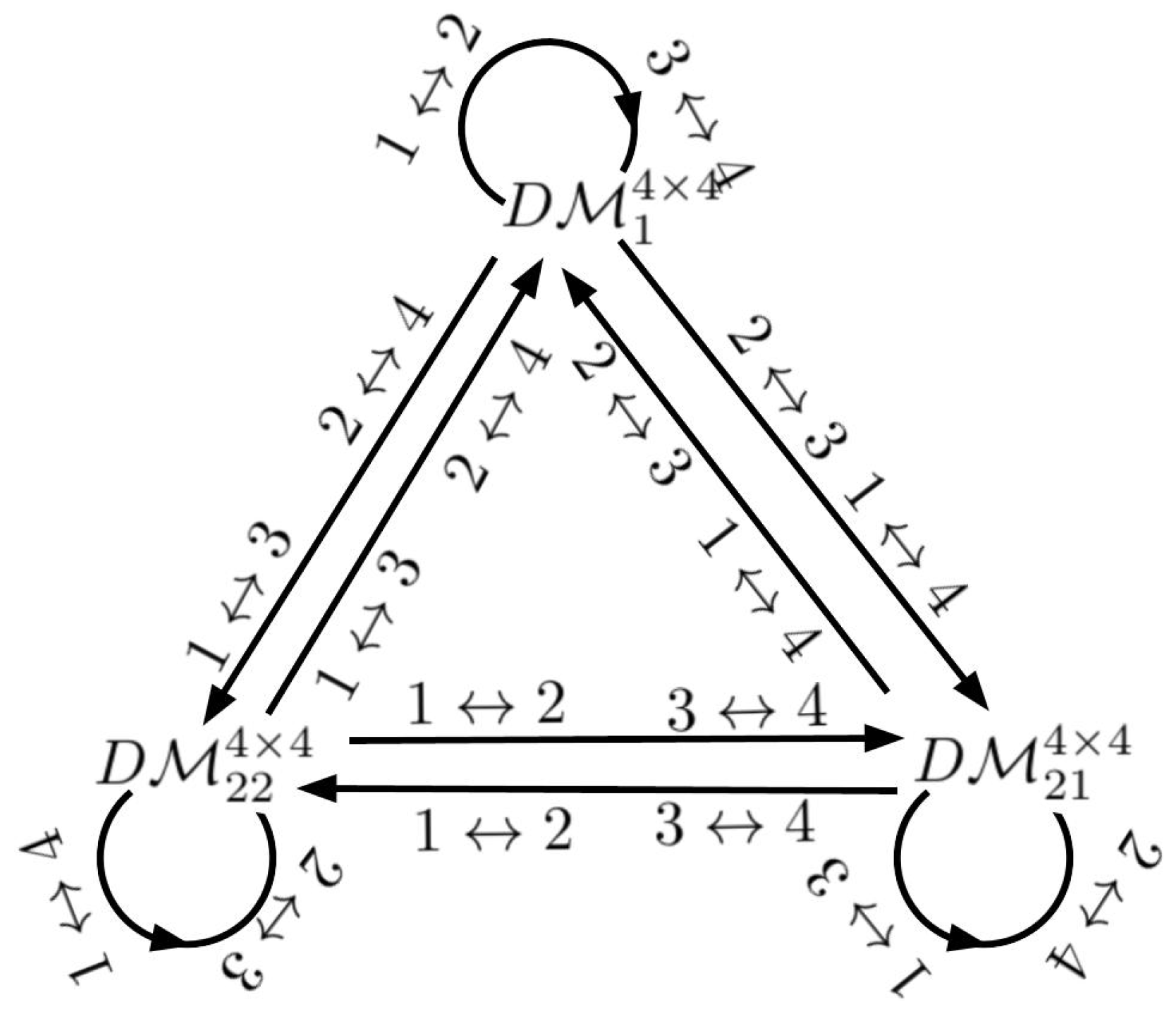
Any associated metric matrices with four concyclic points are linearly independent.

Proof. 

Let $A,B,C,D$ be four arbitrary points on a given circle, as shown in Figure 3. Per Ptolemy’s Theorem [8], the lengths of edges abide by

$$\begin{array}{c}\hfill \overline{AB}\times \overline{CD}=\overline{AD}\times \overline{BC}+\overline{AC}\times \overline{BD}.\end{array}$$

(34)

Figure 3. Concyclic points [9] on a given circle with some center and radius; $A,B,C,D$ are four chosen representative points and $E_1,E_2,\cdots ,E_N$ comprise a dataset with a relation to the representative points that is to be calculated. Solid lines indicate the distances between representative points, and their length serves as a basis for other distances. The solid dots right along the circle are used to indicates the possible positions for other $E_j$ points. The dashed lines are the distances between ${\left\{E_j\right\}}_{j=1}^N$ and the four representative points.

Let $\mathcal{D}=\left[\begin{array}{cccc}0& \overline{AB}& \overline{AC}& \overline{AD}\\ \overline{AB}& 0& \overline{BC}& \overline{BD}\\ \overline{AC}& \overline{BC}& 0& \overline{CD}\\ \overline{AD}& \overline{BD}& \overline{CD}& 0\end{array}\right]$; if $\left|\mathcal{D}\right|=0$, then per Lemma 1 we have

$$\begin{array}{c}\hfill \overline{AB}\times \overline{CD}=\overline{AC}\times \overline{BD}+\overline{AD}\times \overline{BC}\pm 2\sqrt{\overline{AC}\times \overline{AD}\times \overline{BC}\times \overline{BD}}.\end{array}$$

(35)

Comparing Equation (34) with (35), we have $\overline{AC}\times \overline{AD}\times \overline{BC}\times \overline{BD}=0$, which is a contradiction. Therefore, $\left|\mathcal{D}\right|\ne 0$, i.e., $\left\{\left[\begin{array}{c}0\\ \overline{AB}\\ \overline{AC}\\ \overline{AD}\end{array}\right],\left[\begin{array}{c}\overline{AB}\\ 0\\ \overline{BC}\\ \overline{BD}\end{array}\right],\left[\begin{array}{c}\overline{AC}\\ \overline{BC}\\ 0\\ \overline{CD}\end{array}\right],\left[\begin{array}{c}\overline{AD}\\ \overline{BD}\\ \overline{CD}\\ 0\end{array}\right]\right\}$ could serve as a basis for other points on the circumsphere of the given circle. □

Based on Claim 7, we can analyze a dataset. Given a dataset ${\left\{E_j\right\}}_{j=1}^N$, we can compute each distance column matrix ${\mathsf{\Sigma }}_j\equiv [\overline{E_{j}A},\overline{E_{j}B},\overline{E_{j}C},\overline{E_{j}D}]$. Then, the set of distances (or coordinates) between the dataset ${\left\{E_j\right\}}_{j=1}^N$ and the four representative points $A,B,C,D$ can be calculated as ${\left\{{\mathcal{D}}^{-1}{\Sigma }_j\right\}}_{j=1}^N$. This set provides us with some information about the dataset in terms of the distances between representative points.

Example 3.

Given a 2D unit circle with origin $\overrightarrow{0}\equiv (0,0)$ and eight uniformly sampled points ${\{{\overrightarrow{P}}_n=(cos{\displaystyle \frac{n}{4}}\pi ,sin{\displaystyle \frac{n}{4}}\pi )\}}_{n=1}^8$, $A,B,C,D$ are respectively associated with ${\overrightarrow{P}}_4,{\overrightarrow{P}}_8,{\overrightarrow{P}}_6,{\overrightarrow{P}}_3$, while $E_1$, $E_2$, $E_3$, $E_4$ are respectively associated with ${\overrightarrow{P}}_1,{\overrightarrow{P}}_2,{\overrightarrow{P}}_5,{\overrightarrow{P}}_7$. After a series of calculations, the following results are obtained:

$\mathcal{D}=\left[\begin{array}{cccc}0& \overline{AB}& \overline{AC}& \overline{AD}\\ \overline{AB}& 0& \overline{BC}& \overline{BD}\\ \overline{AC}& \overline{BC}& 0& \overline{CD}\\ \overline{AD}& \overline{BD}& \overline{CD}& 0\end{array}\right]=\left[\begin{array}{cccc}0.00& 2.00& 1.41& 0.77\\ 2.00& 0.00& 1.41& 1.85\\ 1.41& 1.41& 0.00& 1.85\\ 0.77& 1.85& 1.85& 0.00\end{array}\right]$; $\left|\mathcal{D}\right|=-11;\left[\begin{array}{cccc}\overline{E_{1}A}& \overline{E_{2}A}& \overline{E_{3}A}& \overline{E_{4}A}\\ \overline{E_{1}B}& \overline{E_{2}B}& \overline{E_{3}B}& \overline{E_{4}B}\\ \overline{E_{1}C}& \overline{E_{2}C}& \overline{E_{3}C}& \overline{E_{4}C}\\ \overline{E_{1}D}& \overline{E_{2}D}& \overline{E_{3}D}& \overline{E_{4}D}\end{array}\right]\equiv [{\sum }_1,{\sum }_2,{\sum }_3,{\sum }_4]=\left[\begin{array}{cccc}1.85& 1.41& 0.77& 1.85\\ 0.77& 1.41& 1.85& 0.77\\ 1.85& 2.00& 0.77& 0.77\\ 1.41& 0.77& 1.41& 2.00\end{array}\right]$. Hence, the distances between $\{E_1,E_2,E_3,E_4\}$ and the basis $\mathcal{D}$ can be represented by

${\mathcal{D}}^{-1}[{\sum }_1,{\sum }_2,{\sum }_3,{\sum }_4]=\left[\begin{array}{cccc}0& 0& 0.54& 0\\ 0.77& 0.41& 0& 0.54\\ 0& 0& 0.54& 0.54\\ 0.41& 0.77& 0& 0\end{array}\right].$

5. Conclusions

It is interesting to know the boundary between linear independence and metric matrices. In this article, we study the dependence and independence of metric matrices based on some algebraic calculations related to the triangle inequality. This study concludes that the set of all 4-by-4 metric matrices, or ${\mathcal{M}}^{4\times 4}$, can be characterized by a set of disjoint metric matrices, or more precisely by ${\mathcal{M}}^{4\times 4}=({\mathcal{M}}^{4\times 4}-D{\mathcal{M}}^{4\times 4})\cup D{\mathcal{M}}^{4\times 4}=({\mathcal{M}}^{4\times 4}-D{\mathcal{M}}^{4\times 4})\cup [D{\mathcal{M}}_1^{4\times 4}\cup D{\mathcal{M}}_2^{4\times 4}]=({\mathcal{M}}^{4\times 4}-D{\mathcal{M}}^{4\times 4})\cup [D{\mathcal{M}}_1^{4\times 4}\cup (D{\mathcal{M}}_{21}^{4\times 4}\cup D{\mathcal{M}}_{22}^{4\times 4})]$. This characterization completes the dependence and independence for 4-by-4 metric matrices. In addition, we demonstrate some applications of these results; in particular, we show that certain distance functions are linearly independent. These statements should help to better understand the properties of metrics, especially, their relations to vector spaces.

References

- Deza, M.M.; Deza, E. Encyclopedia of Distances; Springer: Berlin/Heidelberg, Germany, 2016. [Google Scholar]
- Deza, M.M.; Petitjean, M.; Markov, K. Mathematics of Distances and Applications; ITHEA: Sofia, Bulgaria, 2012. [Google Scholar]
- Dokmanic, I.; Parhizkar, R.; Ranieri, J.; Vetterli, M. Euclidean Distance Matrices: Essential theory, algorithms, and applications. IEEE Signal Process. Mag. 2015, 32, 12–30. [Google Scholar] [CrossRef]
- Alfakih, A. Euclidean Distance Matrices and Their Applications in Rigidity Theory; Springer: Cham, Switzerland, 2018. [Google Scholar]
- Guterman, A.E.; Zhilina, S.A. Relation Graphs of the Sedenion Algebra. J. Math. Sci. 2021, 255, 254–270. [Google Scholar] [CrossRef]
- Hennig, C. Minkowski distances and standardisation for clustering and classification on high-dimensional data. In Advanced Studies in Behaviormetrics and Data Science. Behaviormetrics: Quantitative Approaches to Human Behavior; Imaizumi, T., Nakayama, A., Yokoyama, S., Eds.; Springer: Singapore, 2020; Volume 5, pp. 103–118. [Google Scholar]
- Gao, C.X.; Dwyer, D.; Zhu, Y.; Smith, C.L.; Du, L.; Filia, K.M.; Bayer, J.; Menssink, J.M.; Wang, T.; Bergmeir, C.; et al. An overview of clustering methods with guidelines for application in mental health research. Psychiatry Res. 2023, 327, 115265. [Google Scholar] [CrossRef]
- Indika, G.W.; Amarasinghe, S. A Concise Elementary Proof for the Ptolemy’s Theorem. Glob. J. Adv. Res. Class. Mod. Geom. 2013, 2, 20–25. [Google Scholar]
- Coolidge, J.L. Concurrent Circles and Concyclic Points. A Treatise on the Geometry of the Circle and Sphere; Chelsea: New York, NY, USA, 1971. [Google Scholar]
Disclaimer/Publisher’s Note: The statements, opinions and data contained in all publications are solely those of the individual author(s) and contributor(s) and not of MDPI and/or the editor(s). MDPI and/or the editor(s) disclaim responsibility for any injury to people or property resulting from any ideas, methods, instructions or products referred to in the content. |
© 2024 by the author. Licensee MDPI, Basel, Switzerland. This article is an open access article distributed under the terms and conditions of the Creative Commons Attribution (CC BY) license (https://creativecommons.org/licenses/by/4.0/).