The Geometry of Dynamic Time-Dependent Best–Worst Choice Pairs

Abstract

There has been increasing interest in best–worst discrete choice experiments (BWDCEs) in health economics, transportation research, and other fields over the last few years. BWDCEs have distinct advantages compared to other measurement approaches in discrete choice experiments (DCEs). A systematic study of best–worst (BW) choice pairs can be traced back to the 1990s. Recently, new ideas have been introduced to the subject. Calculating utility helps measure the attractiveness of BW choices. The goal of this paper is twofold. First, we extend the idea of the BW choice pair to include dynamic, time-dependent transition probability and capture utility at each time and for each choice pair. Second, we used the geometry of BW choice pairs to capture the correlations among them and to characterize and clarify the BW choice pairs in the network, where properties can be derived within each class. This paper discusses BWDCEs, the probability transition matrix of choices over time, and the utility function. The proposed network classification for BW choice pairs is laid out. A detailed simulated example is presented, and the results are compared with the classical $\mathbf{K}$-means classification.

1. Introduction

Modeling and classifying human choice behaviors is always a very challenging part of statistical research. Discrete choice experiments (DCEs) provide tools that can be used to elicit these choice behaviors and preferences. According to [1], it has been stated that when the choices are complete, they are made under a justifiably expected utility representation with a probability distribution in which the expected utility increases in the next time period. See [2] for an example. The utility is defined as a function of time and the systematic component from the covariates, which is called attributes and their levels (attribute levels). The best–worst discrete choice experiments (BWDCEs) are specially designed to reveal the respondent’s best and worst choices (see [2]). These approaches began in marketing, and the majority of their applications can be found in the transportation and health literature as well. The design for BWDCEs is more efficient than the full factorial design. An efficient design algorithm selects only a few choice pairs (see [3,4]).

There are three different cases identified in BWDCEs (see [5]). They are called best–worst scaling (BWS) methods. In BWS Case 1 experiments (see [6]), respondents are asked to recognize the most (best) and the least (worst) important attributes without focusing on the actual attribute levels, while in BWS Case 2, experiments (see [7]) require respondents to recognize the most (best) and the least (worst) important attribute level. The BWS Case 3 surveys require respondents to identify both the best and the worst desired alternative in each choice (see [8]).

Experimenting with several choices or choice sets may cause a cognitive burden on respondents (see [9]). A framework is needed to understand the utility parameters associated with the choices for robust predictions under computational simulations before applying them to real data. Additionally, experimenters do not recommend using full factorial designs, as they generally involve a large number of choice sets. Instead, fractional factorial designs such as orthogonal main effect plans (OMEPs) become more tractable and manageable. In the OMEP, only selected alternatives for each attribute in a choice set are available. Note that although it helps to overcome respondents’ mental fatigue, some important characteristics within a choice set may be lost. OMEP is commonly used to distinguish and quantify utilities. It reveals the utilities of the choices. However, OMEPs may not be feasible for large combinations of attributes and attribute levels (see [10]). Moreover, under the OMEP, identifying the network of choice behaviors may reveal choice classification based on utilities over time and build a dynamic time-dependent framework of the BWDCEs. Such a classification has not been introduced in the literature for DCEs. The classification and networking of choice behaviors is computationally challenging because of the correlation induced by the transition in the choice selection in time and limited covariates.

The novelty in this manuscript is in the proposed network classification model based on the theory of convex geometry called “betaMix” (see [11]). In the “betaMix” model, choices that share the linkage are connected into a topology (tessellation) and create classification groups based on their utility values. The understanding of the BW choice pairs comes out clearly in a graphical display as paths and edges describe a possible transition between BW choice pairs. Comparisons with the well-known $\mathbf{K}$-means classification method are made, and the advantages of the convex geometry approach of making the network of choices are highlighted.

The paper is organized as follows. Section 2 describes the BWDCEs. Section 3 presents the probability transition matrix of choices over time, the utility function, and the proposed network classification for best–worst choice pairs. In Section 4, a detailed simulated example is presented. The discussion is provided in Section 5, and the conclusion is in Section 6. Finally, future works and improvements are mentioned in Section 7.

2. Materials and Methods

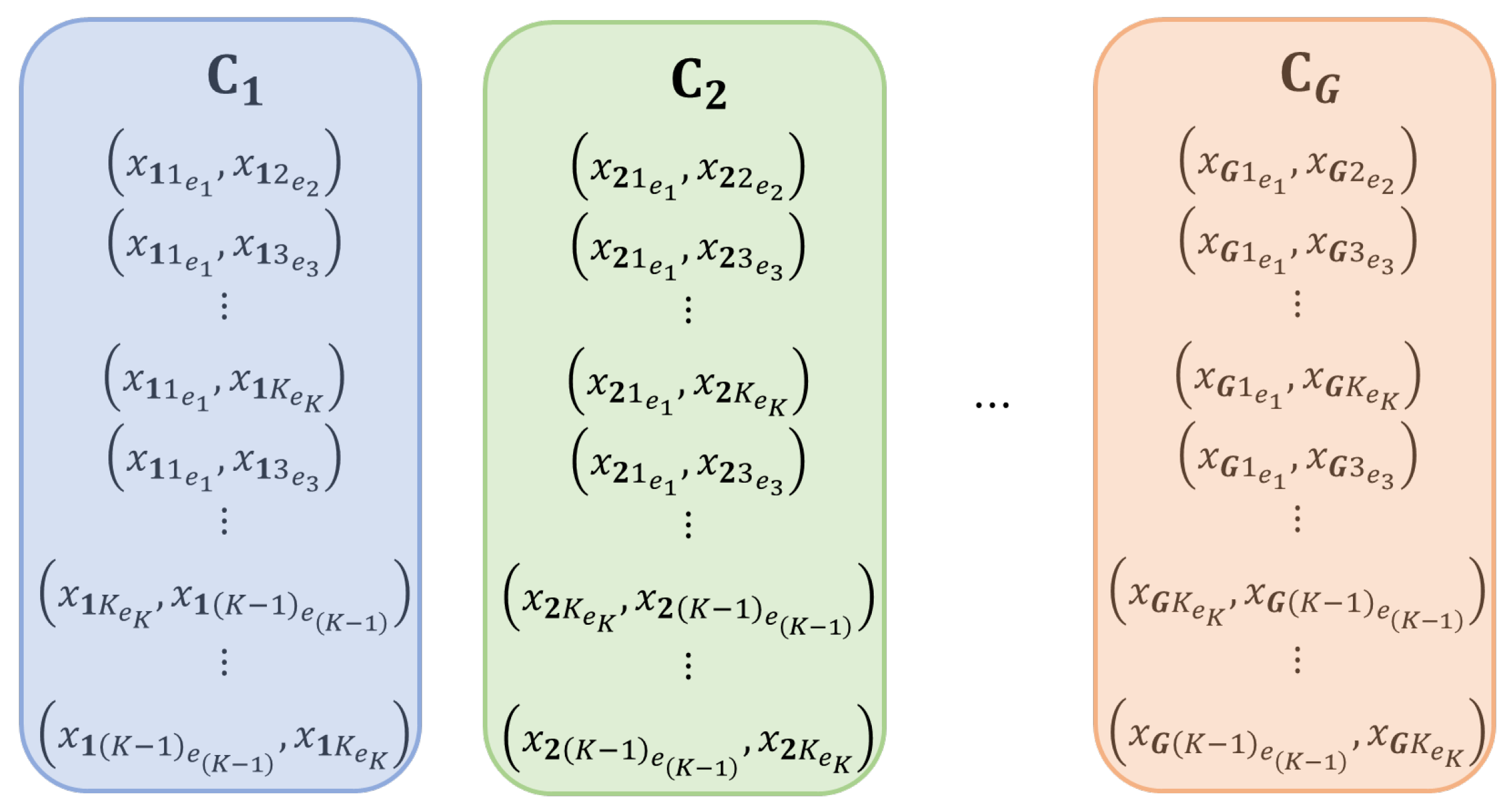
2.1. Best–Worst Discrete Choice Experiments

Modeling choice behaviors has always been a challenging part of statistical study and surveys. In the BWDCEs, as shown in [12], respondents are expected to make choices between different attributes (alternatives). In such experiments, a product or service is described by a set of K attributes. Each attribute contains $l_k$ levels, where $k=1,\dots ,K$. Let us consider an example in a transportation choice scenario (see [5]). Assume that connection time is an attribute with five levels: 2.5 h (conn150), 3 h (conn180), 3.5 h (conn210), 4.5 h (conn270) and 5.5 h (conn330). If we combine the attribute and attribute levels, we have a profile denoted as $X=(x_{1_{e_1}},x_{2_{e_2}},\dots ,x_{K{e}_K})$, where $x_{k_{e_k}}$ is the $e_k^{th}$ level of the $k^{th}$ attribute and each $x_k$ has a total of $l_k$ levels, where $l_k\in \mathbf{N}$ and $k=1,2,\dots ,K$. Then, the pair $(x_{b_{e_b}},x_{w_{e_w}})$ represents a BW choice pair, where $x_{b_{e_b}}$ is the best and $x_{w_{e_w}}$ is the worst, $b\ne w;b,w=1,2,\dots ,K$. Respondents are choosing BW choice pairs from a choice set $C_X=\{(x_{1_{e_1}},x_{2_{e_2}}),\dots ,(x_{1_{e_1}},x_{K_{e_K}}),(x_{2_{e_2}},x_{1_{e_1}}),\dots (x_{2_{e_2}},x_{K_{e_K}}),\dots ,(x_{K_{e_K}},x_{1_{e_1}}),\dots ,(x_{K_{e_K}},x_{{(K-1)}_{e_{(K-1)}}})\}$. Consider an example of $K=3$ attributes $A,B,C$ with each attribute as $l_k=3$ levels, for all $k=1,2,3$, where attribute A has $a_1,a_2,a_3$ levels, B has $b_1,b_2,b_3$ levels and C has $c_1,c_2,c_3$ levels. The number of possible profiles is given by ${\displaystyle \prod _{k=1}^K{l}_k}$. There are 27 profiles in this scenario, and $X=(a_1,b_3,c_2)$ is an element for a set of 27 profiles. Then, the corresponding choice set is $C_X=\{(a_1,b_3),(a_1,c_2),(b_3,a_1),(b_3,c_2),(c_2,a_1),(c_2,b_3)\}$. The number of possible pairs per choice set is $\tau =6.$ The set candidate of profiles is an array. When each pair of attributes and attribute levels appears with the same frequency, the array is called orthogonal. Orthogonal arrays (OAs) are applied usually on a small subset of choice sets or in the OMEP. The extension with time dependence is presented next. The computations of the model parameters are based on the OA coding.

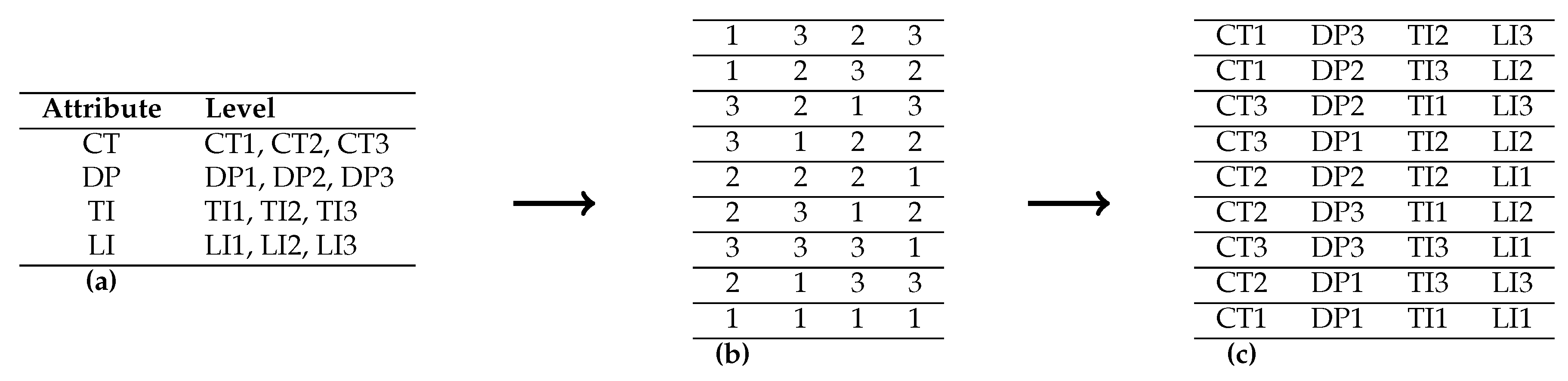
2.2. Design of Experiment

The full factorial designs are usually not practical due to the large number of attributes and attribute levels. Instead, partial factorial designs are more tractable and more informative in the survey designs. We used OMEPs to construct profiles using an orthogonal array (OA) (see [13,14]). These fractional factorial designs are effective and interpretable. They provide sufficient information to estimate parameters (see [4,15,16,17]). Let G be the number of profiles constructed using an OA, such that each profile contains all of the attributes and attribute levels from each attribute, which is selected in an orthogonal way. Assume that the profiles have K attributes and each attribute has $l_k$ levels $k=1,2,\dots ,K$. If all the attributes have the same number of levels, l, a $l^K$ OA is used to construct the profiles. From the G profiles, we obtain $X_1=(x_{{11}_{e_1}},x_{{12}_{e_2}},\dots ,x_{1K{e}_K}),X_2=(x_{{21}_{e_1}},x_{{22}_{e_2}},\dots ,x_{2K_{e_K}}),\dots ,X_G=(x_{G{1}_{e_1}},x_{G{2}_{e_2}},\dots ,x_{G{K}_{e_K}})$, where $x_{g{k}_{e_k}}$ is the $e_k^{th}$ level of the $k^{th}$ attribute from the $g^{th}$ profile. The $k^{th}$ attribute has $l_k$ levels, $l_k\in \mathbf{N}$, the attribute-level $e_k$ is defined in the set $\{1,\dots ,l_k\}$$i.e.$$e_k\in \{1,2,\dots ,l_k\},k=1,2,\dots ,K$ and $g=1,2,\dots ,G$.

An application with the transportation attribute and attribute levels is presented in Section 3. In general, if we combine the choice sets, we can define W, where $W=(C_1,C_2,\dots ,C_G)$ such that $C_i\ne C_j$ for all $i\ne j$; $i,j=1,2,\dots ,G$. The G choice sets are illustrated in Figure 1. In each of the choice sets, there are $\tau =K(K-1)$ BW choice pairs. The experiment is conducted so that all respondents must choose from each of the G choice sets. Each choice set maps into the corresponding profile. In building inferences based on the utility functions of the choice pairs over time, challenges are due to the distributional assumptions and the ordinal ranking (importance) in the choice pairs.

2.3. Utility Function

Choices are made under the assumption of utility maximization or random utility theory (see [18]). Many authors, such as McFadden [19], Flynn et al. [7,20], and Louviere et al. [21], provided the utility function for best–worst choice models. The choice set is described so that the respondent’s utility is maximized among the $\tau$ choice pairs in a considered choice set. The utility function as described in [19] for a consumer selecting the $j^{th}$ choice is given as

$$U_j=V_j+{ϵ}_j,$$

(1)

where $U_j$ is the utility for selecting the $j^{th}$ choice, and $V_j$ captures the systematic component of that choice and ${ϵ}_j$ captures the error component, $j=1,\dots ,\tau$.

The error terms are independently and identically Gumbel distributed as presented in [19]. As in [17], we assume the respondents are independent, but their preferred choices are not. Under random utility theory, respondents pick choices with the highest utility values [22].

As mentioned in Section 2.1, let $(x_{i{b}_{e_b}},x_{i{w}_{e_w}})$ be the chosen pair for the ${e_b}^{th}$ level of the $b^{th}$ attribute as the best choice and the ${e_w}^{th}$ level of the $w^{th}$ attribute as the worst choice. Let us use $(x_{ij},x_{i{j}^{\prime }})$ as the chosen pair for the $j^{th}$ best attribute, attribute-level and the $j^{\prime th}$ worst attribute, attribute-level from the $i^{th}$ choice set $\left(C_i\right)$, as in Figure 1, for the sake of notational simplicity, where $j\ne j^{\prime },j,j^{\prime }=1,2,\dots ,K$ and $i=1,2,\dots ,G$. Then, the utility for choosing the pair $(x_{ij},x_{i{j}^{\prime }})$ is given by

$$U_{ij{j}^{\prime }}=V_{ij{j}^{\prime }}+{ϵ}_{ij{j}^{\prime }},$$

(2)

where $U_{ij{j}^{\prime }}$ is the random utility value of selecting the $j^{th}$ choice as the best and the $j^{\prime th}$ choice as the worst from the $i^{th}$ choice set with systematic component $V_{ij{j}^{\prime }}$, and the error term ${ϵ}_{ij{j}^{\prime }}$ follows a logistic distribution [23]. Here, the term “choice” is used for choosing the attribute and attribute level within the $i^{th}$ choice set. The systematic component $V_{ij{j}^{\prime }}=M\mathbf{\beta }$, where the $\beta$’s are the estimated regression coefficients, and M is the design matrix for any choice set. M is composed based on the model we choose. In this manuscript, we use the paired model to construct M (see [14]), which assumes that the difference in utility between the two levels represents the greatest utility difference among all $\tau$ utility differences for a choice set (see the example in [7]).

3. Theory of Choice Transition and Classification

3.1. Transition Probability

Choice alternatives are not mutually exclusive over time. If we assume the decision process is Markovian, the transition probability to the next state (choice pair), $s^{\prime }:=s_{t+1}$ based solely on the decision made at the current state, $s:=s_t$ is $P_{s{s}^{\prime }}=P[s_{t+1}=s^{\prime }|s_t=s]$, where $t=1,\dots ,T$ and $s,s^{\prime }$ are among the $\tau$ choice pairs. Here, s represents the state selected at the current time t, while $s^{\prime }$ denotes the state selected at the next time point $t+1$. Hence,

$$P\left(s_{t+1}\right|s_t)=P(s_{t+1}=s^{\prime }|s_t=s)=P_{s{s}^{\prime }},$$

(3)

denotes the conditional probability of state transition from s to $s^{\prime }$, where $s,s^{\prime }=1,2,\dots ,\tau$ (see [19,24] for derivations). A time-dependent formula to calculate the transition probability based on the conditional logit model assumption (see [19]) of the utility function was established by Working [2] and Adikari and Diawara [25]. In this paper, we introduce copula distribution with a CUB (combination of discrete uniform and shifted binomial distributions) marginal, extending the work by Piccolo [26] to construct more flexible choice transition probabilities. The novelty is this new approach to discrete choice modeling makes it possible to introduce a priority constraint $|s^{\prime }-s|\le \delta$ based on the assumption that a customer has a greater tendency to grab options close at hand or those within the nearest range rather than picking up alternatives further away in time, where $\delta$ is an arbitrary integer (the value of $\delta$ can be decided based on the past experience of the product/service). Then, the transition probability model can be stated as follows:

$$P\left(s^{\prime }\right|s)=\left\{\begin{array}{cc}{\displaystyle \frac{c_{\theta }(s,s^{\prime })}{P\left(s\right)}}{\displaystyle \frac{n_{s{s}^{\prime }}}{d_s}},\hfill & d_s\ne 0\mathtt{and}|s^{\prime }-s|\le \delta \hfill \\ 0,\hfill & d_s=0\hfill \end{array},\right.$$

(4)

where $s\sim P\left(s\right)=CUB(m,\pi ,\xi )$, $s^{\prime }\sim P\left(s^{\prime }\right)=CUB(m,{\pi }^{\prime },{\xi }^{\prime })$, and $d_s$ is the sum of the $P\left(s^{\prime }\right|s)\times n_{s{s}^{\prime }}$ portion for each s, where $s,s^{\prime }=1,2,\dots ,\tau$, and $(s,s^{\prime })\sim C_{\theta }(u_{\pi ,\xi },v_{{\pi }^{\prime },{\xi }^{\prime }})$; $u,v$ are cumulative mass functions of CUB.

The probability mass function of CUB is

${\displaystyle P(R=r)=\pi \left(\genfrac{}{}{0pt}{}{m-1}{r-1}\right){\xi }^{m-r}{(1-\xi )}^{r-1}+(1-\pi )\frac{1}{m},}$

where $r=1,2,\dots ,m;\pi \in (0,1];\xi \in (0,1]$ (see [26,27]).

Here, $C_{\theta }$ is the bivariate placket copula distribution. There can be repetitions among choice pairs selections. Therefore, an adjustment must be made to retain it as a probability model.

The entry ${\displaystyle \frac{c_{\theta }(s,s^{\prime })}{P\left(s\right)}}$ needs to be multiplied by term ${\displaystyle \frac{n_{s{s}^{\prime }}}{d_s}}$, where $n_{s{s}^{\prime }}$ is the number of transitions from choice state s to $s^{\prime }$ (repetitions). Then, the transition probability from s to $s^{\prime }$, $P\left(s^{\prime }\right|s)\in [0,1]$. For the imposed priority constraint $|s^{\prime }-s|\le \delta$, $\delta =1,2,\dots ,\tau$. In the examples, we take $\delta =2.$

The use of copula distribution arises for flexibility while accounting for the constraint. Picollo [26] and D’Elia and Piccolo [27] offered some aspect of the dynamic of discrete choice modeling, but time was not added. There are many rows (optional BW choices) in the transition matrix. To make use of stationarity and avoid singularity issues, the entries are non-negative and must add up to 1 if that choice is selected or 0 otherwise (see [25]). Stability and convergence in the process are needed properties. In this work, the focus is on a simple presentation in which the geometry of BW choice pairs applies.

The initial utility for each choice is calculated using Equation (2). The utility over time is calculated by using a backward recursive method called Bellman’s equation (see [28,29]):

$$V_t(s_t,{ϵ}_t)=\underset{d_t\in D}{max}\sum _{n=t}^{T}P\left(s\right|s^{\prime })[{\gamma }^{n-t}U(s_n,d_n)+ϵ\left(d_n\right)|s_t],$$

(5)

where $P\left(s\right|s^{\prime })$ is the probability transition matrix, $U(s_t,d_t)$ is the initial utility at time t, and $ϵ$ is the associated error term at time t; $t=1,2,\dots ,T$. One cannot assume that a person’s perceived utility is not impacted by time. Therefore, to adjust for the impact of time on the expected utility, a discount rate $\gamma \in (0,1)$ is considered (see [30]). Computed utilities for 15 time points using numerical steps for simulated choice pairs are provided in the application section. Then, the network associated with the BW choice pairs is presented.

3.2. Network Classification Methodology

Having all the BW choice pairs, classification based on the utility becomes very useful. We used the convex geometrical method and $\mathbf{K}$-means methods to build the network and classification diagrams based on utility values for each choice, which are evaluated over time. The two methods will be contrasted.

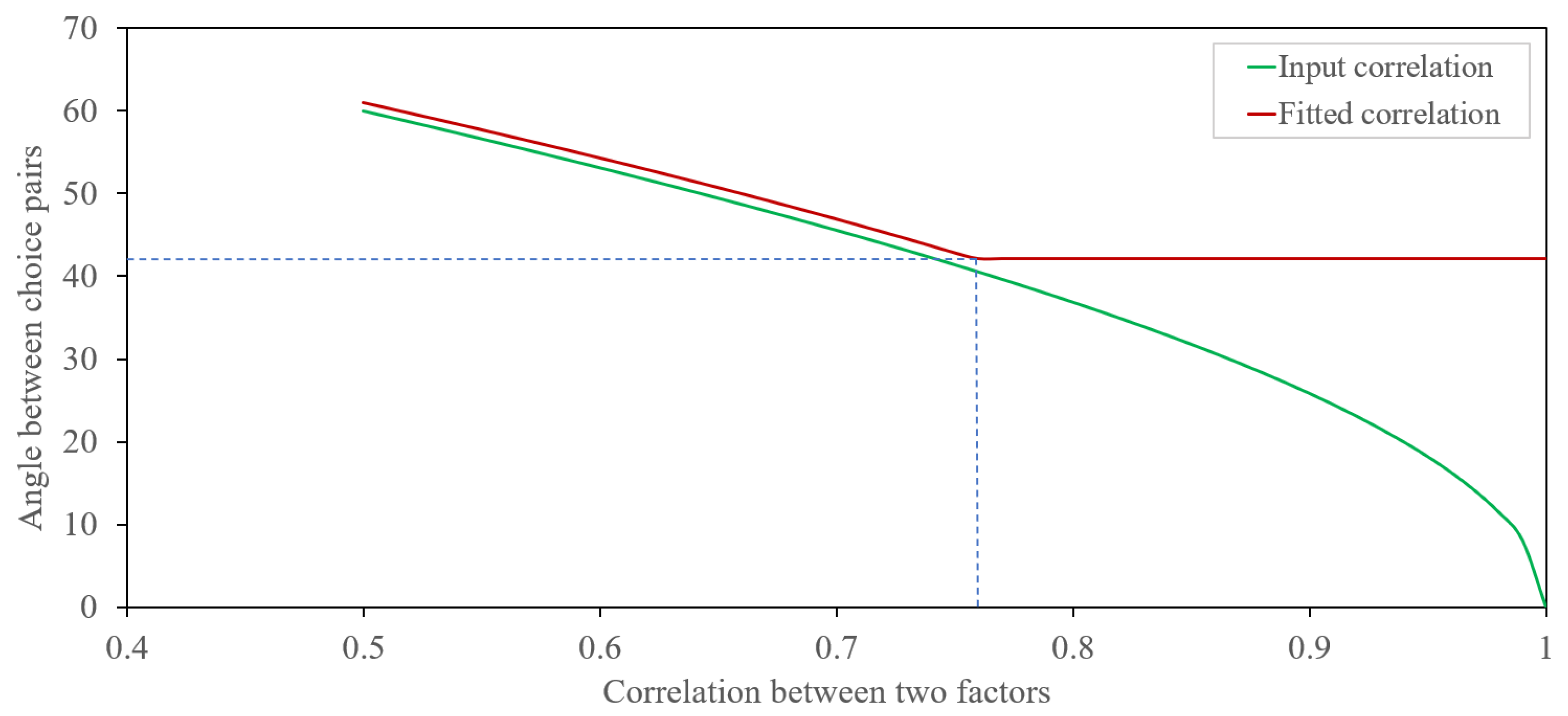
3.3. Convex Geometry Method for Classification

Bar and Wells [11] introduced a mixture model of beta distributions to identify significant correlations predictors called “betaMix”. The method relies on theorems in convex geometry. This classification method does not need any assumptions about the network structure nor does it assume that the network is sparse. Our only assumption here is that the variables (choice pairs) are drawn from a spherically symmetric distribution. This method calculates all the pairwise correlations of the utility of BW choice pairs and finds all the connections between them. The key to this method is “flipping” the roles of variables and observations and treating the data as P points in ${\mathbf{R}}^n$ so that each predictor is characterized by a sample of size n. Ideas from convex geometry have been applied in the statistics literature to developing thresholds for detecting significant edges of the network diagram. In correlation screening, the objective is to select variables whose maximal correlation exceeds a given threshold. Cai and Jiang [31,32]) and Cai et al. [33] took this approach to screening correlations via the analysis of discovering minimal pairwise angles. Bar and Bang [34] considered a mixture model for detecting significant correlations. Their approach relied on Fisher’s Z-transformed correlations and their asymptotic normal distribution under the null hypothesis. This method performs well especially when n is sufficiently large. The important fact about “betaMix” is that it does not require a normalizing transformation, and controlling the error rate relies on a general convex geometry theory. Since it does not require defining one of the variables as the response, we can use it as an unsupervised classifier. The techniques developed in [11] are extended and applied in the context of BW choice pairs for n time points and P unique BW choice pairs.

Frankl and Maehara [35] proved that the if two vectors in $R^n$ are drawn from a multivariate normal distribution, and $\theta$ is the random angle formed between them, then $si{n}^2\left(\theta \right)$ has a beta distribution:

$$Z=si{n}^2\theta \sim Beta({\displaystyle \frac{n-1}{2}},{\displaystyle \frac{1}{2}}),$$

(6)

where $\theta$ is the angle between two BW choice pairs. Hence, an asymptotic approximation for the cumulative distribution function of $\theta$ that holds for any angle $\alpha \in (0,\pi /2)$ is given by

$$P[\theta \le \alpha ]=P[Z\le si{n}^2\alpha ]\approx {\left[{(\pi (n-1)/2)}^{1/2}cos\alpha \right]}^{-1}{\left(sin\alpha \right)}^{n-1}.$$

Absil et al. [36] gave the density of the largest principal angle between two random subspaces. Bar and Wells [11] used both a frequentist and Bayesian inferential procedure in their approach to detecting edges of the network. The edges depend on beta quantiles. Based on the results in [11,35,36], use $z_c<Q_{ϵ}$ as the screening rule for the frequentist approach when detecting an edge in the network diagram of vectors, where $Q_{ϵ}$ denotes the $ϵ$ quantile of $Beta({\displaystyle \frac{n-1}{2}},{\displaystyle \frac{1}{2}})$, ${\theta }_c$ is the angle between the $c^{th}$ pair of BW choices; $c=1,\dots ,P(P-1)/2$ and $z_c=si{n}^2{\theta }_c$. Let us consider the scenario with $P=500$ and $n=70$. Then, the total number of possible edges is $P(P-1)/2=124,750$. Let us assume we want to include an edge in the network diagram if the correlation coefficient is at least $0.5$ between the two vectors; that is, the angle between the corresponding pair of vectors is $\theta ={60}^{\circ }$. Then, $z=si{n}^2\theta =0.75$. Then, for $Q_{ϵ}$ to be $0.75$, we can take $ϵ={10}^{-5}$. That is $Q_{ϵ}({\displaystyle \frac{70-1}{2}},{\displaystyle \frac{1}{2}})\approx 0.75$. Further, [11] presented an adjustment to the betaMix model when the n samples are not independent. In the application, we used this betaMix approach to perform classification for choice pairs based on their utility values over time.

3.4. $\mathbf{K}$-Means Method for Classification

In data mining and knowledge discovery, $\mathbf{K}$-means clustering is the most commonly used unsupervised machine learning algorithm for partitioning a given data set into a set of k groups. In $\mathbf{K}$-means clustering, each cluster is represented by its center, which corresponds to the mean of points assigned to the cluster. Because of the large and complex data, its algorithm and implementation performance may drop, and improvements are suggested. The elbow curve method (see [37]) and silhouette score method (see [38]) are popular methods for deciding the optimal number of clusters in a $\mathbf{K}$-means classification diagram. The silhouette score method is a more precise approach, though it is computationally expensive, and it will be utilized in this paper.

4. Results

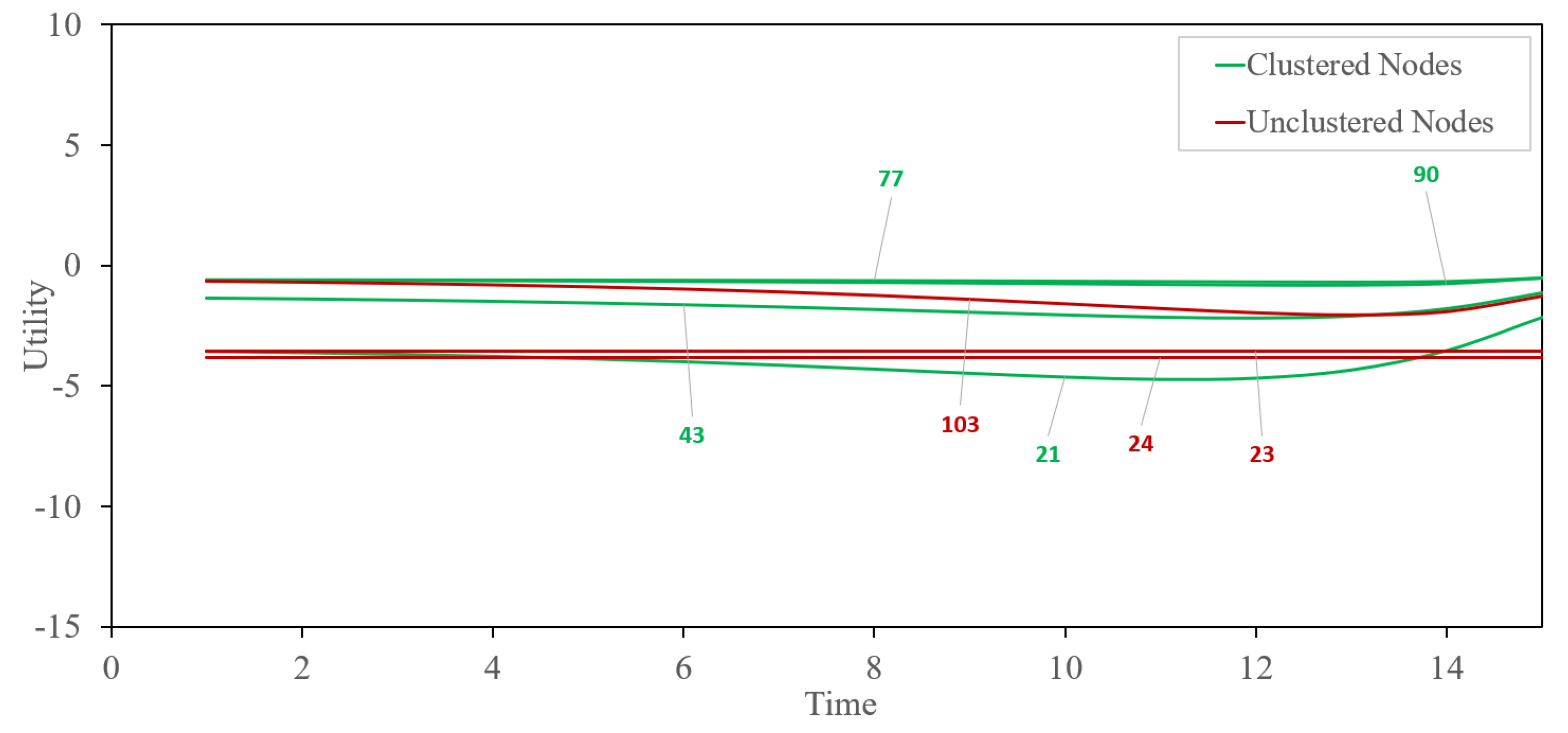
4.1. Geometry of Choice Classification

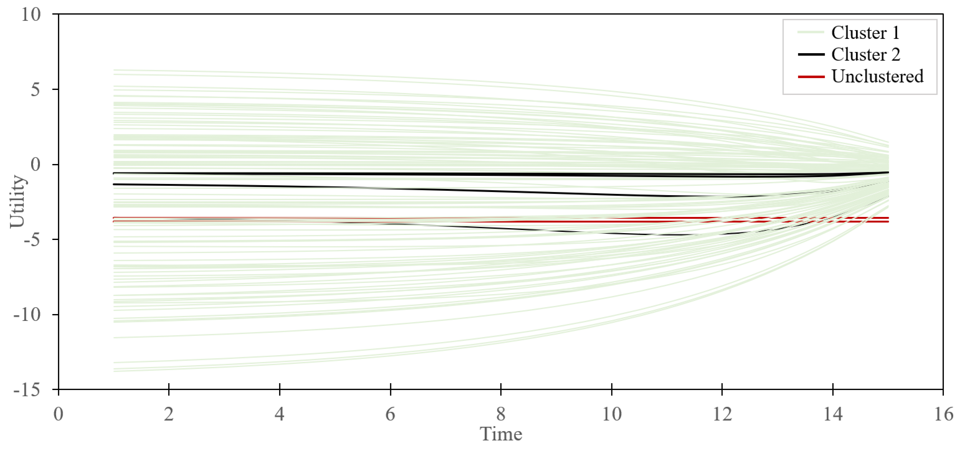
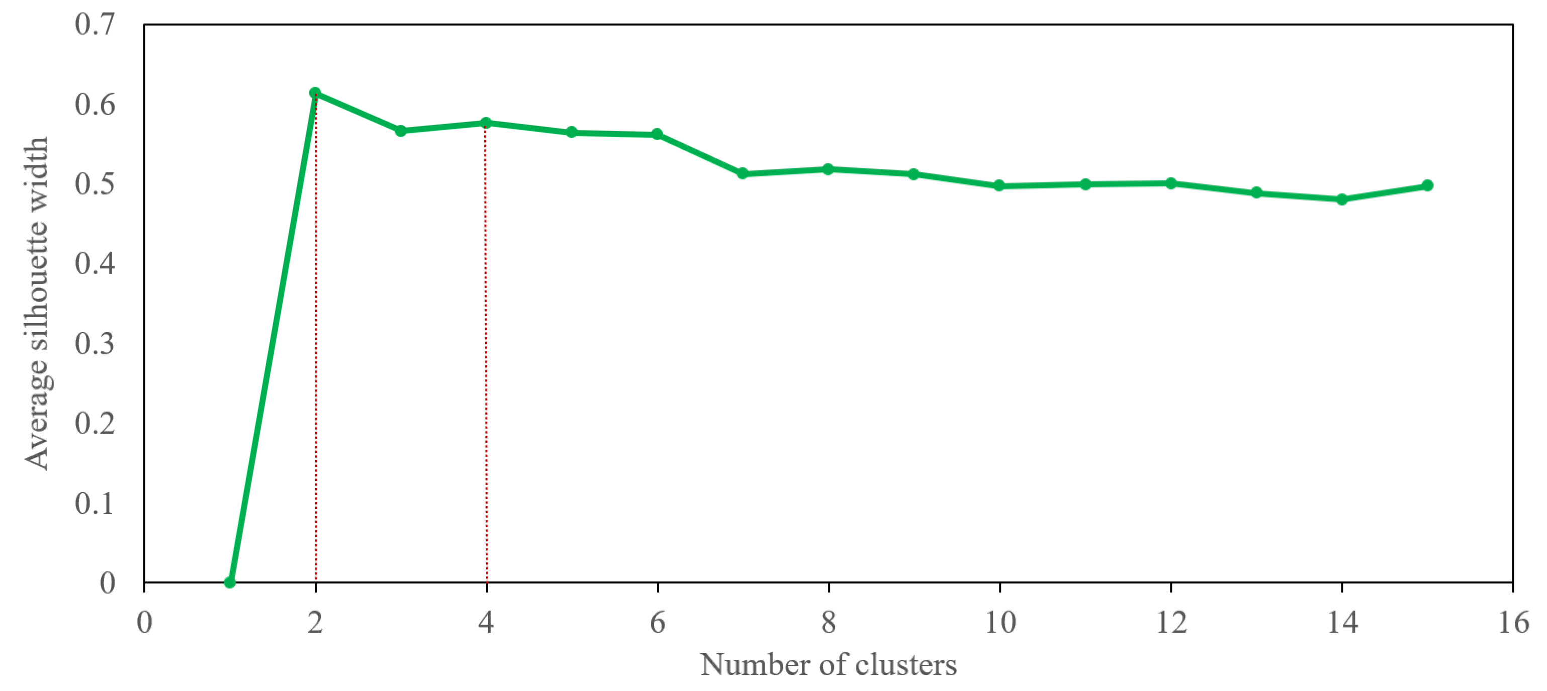
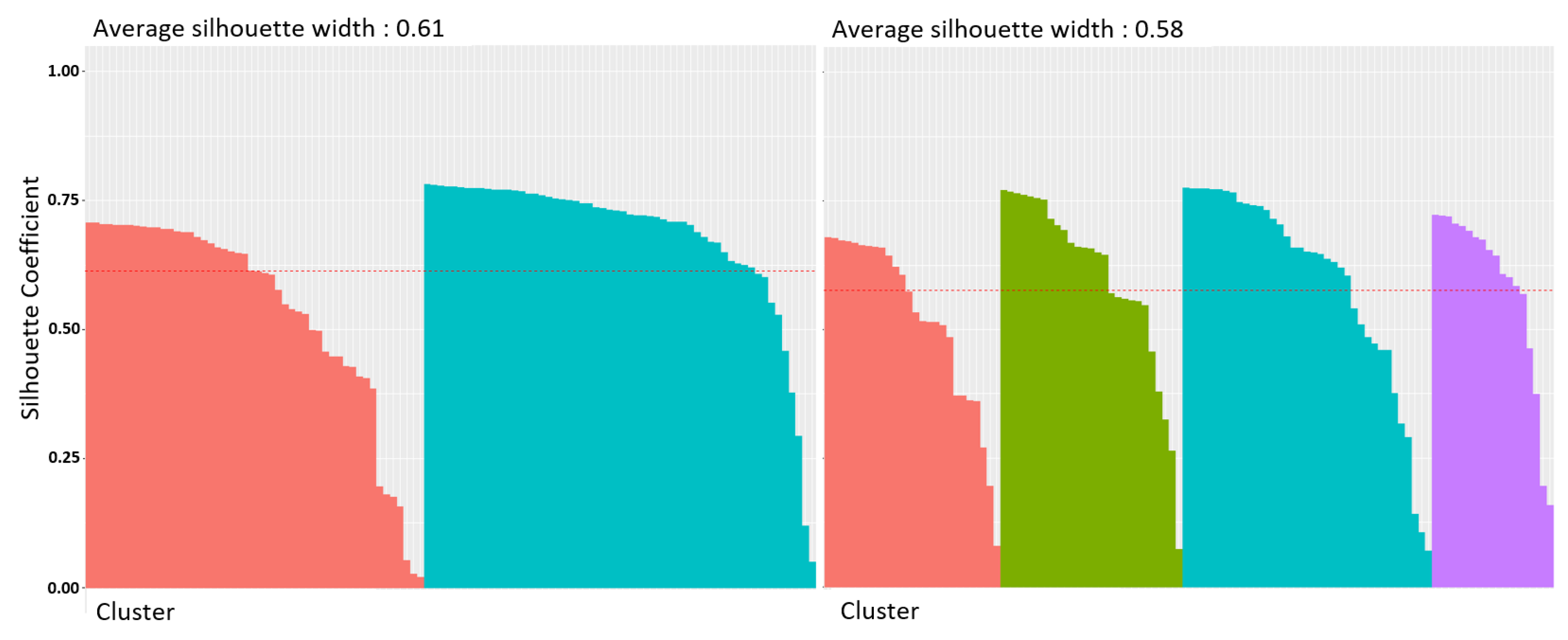
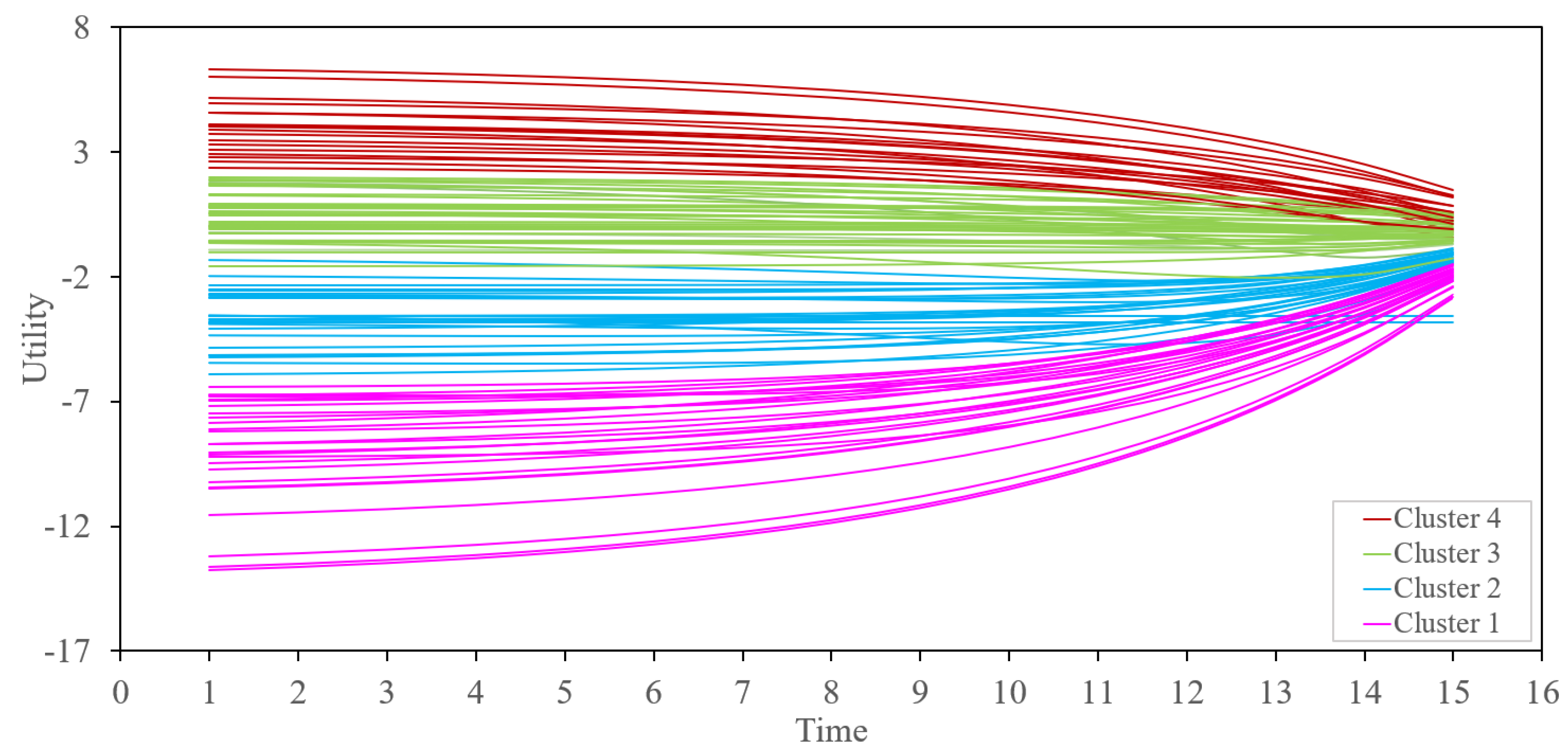
The proposed network is based on the generated data. Our simulation is based on a case study presented in [5]. It is the BW choice case study of integrated high-speed rail service implemented since 2011 in Shanghai, China. They designed the BWS Case 2 experiment in such a way that collected data across four attributes and 14 attribute levels. The data generated adopt ideas from BW scores (see [39]). These scores provide a straightforward implication of attraction of attributes to the consumer. Data simulation is performed with the R package: “support.BWS2”.

This case study has four attributes: connection time (CT), delay protection (DP), ticket integration (TI), and luggage integration (LI). In the original case study, CT has five levels, and DP, TI, and LI have three levels each. We regroup the five levels into three groups for CT to keep three levels each for all four attributes.

By regrouping the five levels into three groups for CT, we were able to ensure that each of the $K=4$ attributes had $l_k=3$ levels, where $k=1,\dots 4$. This allows us to reduce the number of profiles in transportation research and to employ a balanced design for modeling the data. In their analysis, Song et al. [5] calculated the simple BW scores for the main attribute under the BWS Case 1 experiment and analytical BW scores (see [40]) for attribute levels under BWS Case 1 experiment. However, we combined them as one set for the purpose of BW choice pair simulation.

Table 1. BW scores for attributes and attribute-levels.

Attribute	BW Score	Levels	Description	Analytical BW Score
CT (connection time)	0.37	conn180L (CT1) conn180T270 (CT2) conn270M (CT3)	Connection time is less than 3 h Connection time is 3 h to 4.5 h Connection time is more than 4.5 h	$-0.51$ $-0.9$ $-1.27$
DP (delay protection)	0.29	delay0 (DP1) delay1 (DP2) delay2 (DP3)	No delay protection 50% off if major leg missed due to minor leg delay Free change if major leg missed from minor leg delay	$-0.9$ $0.1$ $0.55$
TI (ticket integration)	$-0.47$	tick1 (TI1) tick2 (TI2) tick3 (TI3)	Booked together, no easy collection, fixed-time on minor leg Booked together, easy collection, fixed-time train on minor leg Booked together, each collection, flexible train on minor leg	$0.17$ $0.12$ $0.38$
LI (luggage integration)	0.16	lugg0 (LI1) lugg1 (LI2) lugg2 (LI3)	No luggage integration, checks required on both legs Integrated luggage, checks required on both leg Integrated luggage, one security check required	$-1.02$ $0.57$ $1.22$

shows the attributes, levels, and BW scores.

Hence, when $K=4$ attributes and each attribute has $l_k=3$ levels, $k=1,\dots ,4$, we repeat the analysis, but we need to generate the data first. A simulation of data is performed as follows. The arrangement of a profile is based on an OMEP by using an OA as shown in Figure 2. Figure 2a shows the basic information for each profile. The shortest possible $3^4$ OA (see [41]) is shown in Figure 2b.

Now, set the attributes CT, DP, TI, and LI to be assigned to the first, second, third, and fourth columns of the OA, and let the values 1, 2, and 3 correspond to the level values. By mapping attributes to columns and levels to the integer values, Figure 2c shows the $G=9$ set of profiles. As an example, the 2nd profile is $X_2$ = (CT-conn180L, DP-delay2, TI-tick2, LI-lugg2). Then, we can construct all nine choice sets $(G_1,G_2,\dots ,G_9)$ so that they correspond with each $(X_1,X_2,\dots ,X_9)$ profile. For $k=4$ attributes and $l_k=3$ levels, for all k, $k=1,\dots ,4$, there are 108 unique choice pairs. Therefore, each choice set has $\tau =12$ BW choice pairs (see [25]). We simulated a new data set for 500 individuals. Each person in the sample should make a choice in each choice set. The choice transition probability, that is, the probability of making the next choice at the next time point, is calculated for all 108 choice pairs nested under each choice set using Equation (4). As per the iterative dynamic programming method stated in Equation (5), utility values for $t=15$ consecutive time periods are shown in

Table 2. Utility in time for choices.

Choice Pair	Best Attribute	Worst Attribute	Best Level	Worst Level	Utility at $\mathit{t}=1$	Utility at $\mathit{t}=2$	⋯	Utility at $\mathit{t}=14$	Utility at $\mathit{t}=15$	Choice Set
1	CT	TI	conn180L	tick2	3.098	3.073	⋯	1.339	0.825	1
2	CT	DP	conn180L	delay2	2.802	2.770	⋯	1.067	0.605	1
3	CT	LI	conn180L	lugg2	2.386	2.361	⋯	0.670	0.265	1
⋮	⋮	⋮	⋮	⋮	⋮	⋮	⋯	⋮	⋮	⋮
12	TI	CT	tick2	conn180L	$-11.556$	$-11.450$	⋯	$-4.312$	$-2.395$	1
13	CT	LI	conn180L	lugg1	6.307	6.252	⋯	2.506	1.473	2
14	CT	DP	conn180L	delay1	6.010	5.954	⋯	2.217	1.223	2
15	CT	TI	conn180L	tick3	5.196	5.140	⋯	1.416	0.493	2
⋮	⋮	⋮	⋮	⋮	⋮	⋮	⋯	⋮	⋮	⋮
24	LI	CT	lugg1	conn180L	$-3.807$	$-3.807$	⋯	$-3.807$	$-3.807$	2
25	LI	DP	lugg2	delay1	1.971	1.956	⋯	0.861	0.555	3
26	LI	CT	lugg2	conn270M	1.906	1.890	⋯	0.788	0.475	3
27	LI	TI	lugg2	tick1	1.633	1.617	⋯	0.522	0.235	3
⋮	⋮	⋮	⋮	⋮	⋮	⋮	⋯	⋮	⋮	⋮
85	DP	CT	delay0	conn180T270	1.326	1.318	⋯	0.681	0.445	8
86	DP	TI	delay0	tick3	0.936	0.927	⋯	0.334	0.185	8
87	LI	CT	lugg2	conn180T270	0.766	0.757	⋯	0.202	0.085	8
⋮	⋮	⋮	⋮	⋮	⋮	⋮	⋯	⋮	⋮	⋮
96	CT	DP	conn180T270	delay0	$-9.723$	$-9.634$	⋯	$-3.628$	$-2.015$	8
97	CT	TI	conn180L	tick1	4.972	4.931	⋯	2.100	1.285	9
98	DP	TI	delay0	tick1	4.050	4.009	⋯	1.235	0.955	9
99	CT	LI	conn180L	lugg0	4.011	3.970	⋯	1.155	0.385	9
⋮	⋮	⋮	⋮	⋮	⋮	⋮	⋯	⋮	⋮	⋮
108	TI	CT	tick1	conn180L	$-13.775$	$-13.649$	⋯	$-5.140$	$-2.855$	9

.

We built the network diagram using the betaMix method for the 108 unique choice pairs in the case study. In the network diagram, the nodes represent choice pairs, and the edge represents the significant correlation between the choice pairs. As mentioned in Section 3.3, the screening rule for detecting an edge is $z<Q_{ϵ}$.

Since we need to flip the roles of the number of data points $\left(n\right)$ and the number of variables $\left(P\right)$ as a requirement of the betaMix model, we took n as the number of time points and the number of choice pairs as P such that $n=15$ and $P=108$. Let $ϵ$ be a function of the angle $\left(\theta \right)$ between two choice pairs in the network diagram. The correlation $\left(\rho \right)$ between two nodes (two BW choice pairs) is the same as the cosine value of the angle $\left(\theta \right)$ between two nodes. Therefore, we use $\rho$ as a manual tuning parameter for detecting an edge in the network diagram, which can hardly be found in other unsupervised network classification algorithms. We can fit the betaMix model by adjusting the correlation between two nodes, and we can use the decision parameter to detect an edge to the network diagram. The betaMix model can detect an edge from $\rho =$ 0.76 to 1 for this data set (see Figure 3 and Figure 4). The correlation between two choice pairs is found to be significant with a value of 0.76 or more, e.g., the angle between the choice pairs is about 42 degrees or more. In Figure 3, The green line represents the input correlation of choice pairs, while the red line illustrates how well the fitted beta model captures this correlation.The orange region of Figure 4 shows the fitted range of $si{n}^2\theta$ for which choice pairs are correlated. The green curve represents the null distribution, while the blue curve depicts the fitted model, which closely aligns with the data. Figure 5 shows the network diagram of all the unique BW choice pairs. Cluster 1 has 101 nodes. Only four nodes (choice pair $\#21, 43, 77,$ and 90) are classified in cluster 2. Choice pairs $\#23, 24$ and 103 remain unclustered in the network diagram.

In Figure 6, the utilities of the all the 108 choice pairs are displayed with clusters 1 and 2 and the unclustered group.

Utility–time curves for the nodes classified under cluster 2 and unclassified are shown in Figure 7. As in [5], the DP and LI attributes are favorably selected and attractive. Moreover, having the cluster is allowing us to confirm the indifference. Mainly, choices in the ensemble show that there is a lack of consistency in the choice behaviors as suggested in [5,42], where the sensitivity of the attribute was found as inconsistent in the data. To further the understanding, a comparison with the classical $\mathbf{K}$-means method is added next, which is followed by a discussion.

4.2. $\mathbf{K}$-Means Classification

We used the $\mathbf{K}$-means classification method also to cluster all 108 choice pairs. We used the silhouette score to decide the optimal number of clusters. As we can see in Figure 8, the values $\mathbf{K}=2$ and $\mathbf{K}=4$ are good choices for the selected number of clusters. We can decide the best value for $\mathbf{K}$ by examining the visualization of every instance’s silhouette coefficient, which is sorted by the cluster they are assigned to and by the value of the coefficient (see Figure 9). Based on the silhouette diagram in Figure 9, we can pick $\mathbf{K}=4$ as the optimal number of clusters. See [43,44] for further explanation on clustering by silhouette coefficient. We plot all 108 utilities based on four clusters as shown in Figure 10.

5. Discussion

BW choice pairs with negligible mass under the transition probability distribution are shown at the intersection of the utility–time distribution. When the graph displays disjoint groupings in terms of a large number of utility function BW choice pairs, the $\mathbf{K}$-means algorithm forms some groupings. However, BW choice pairs overlap due to the optimized algorithm’s lack of flexibility in time dependence. In our proposed method, geometry can be used to estimate BW choice pairs with dynamic transition capabilities, and the $\mathbf{K}$-means algorithm can be applied within each cluster obtained for higher stability discrepancies. For two distinct choice pairs, a path or edge is determined between them. From the two distinct times, say 1 and 2, a smaller network effectively emerges, indicating a constant in the discrete transition probability built.

In this paper, we mix time sequence utility values in BW choice pairs from sample paths dictated by transition probabilities.

6. Conclusions

Choices are made in many situations, from healthcare to transportation and more. These decisions are made to maximize some utility function. This paper illustrates the analysis of choice pairs, considering both the best and worst options. Given the dynamic nature of choices, we have proposed and motivated a time-dependent approach to choice pairs. The BW choice pair probability transition is derived under a priority constraint, and the utility values are computed for these pairs. Classification is then proposed based on the geometry of the choice pairs. We illustrate this classification using both simulated and modified aggregated real data with associated dynamic BW choice pairs paths and edges. The results in the transportation example are consistent with literature inference and emphasize the need to build time-dependent choice models. Research on entries in the transition matrix and their associated properties is a formidable task within the constraint of BW choice pairs.

7. Future Works

There are several characterizations that can be made. A variety of transition matrices can be considered at this point under a Markov chain of BW choice pairs. New illustrated graph networks are possible. The quantification and evaluation of the utility function will shed light on the BW choice network. Relating the selected probabilities to the network is an open problem. The random walk option is another matrix option. The question will be how to motivate the choice behaviors.

References

1. Chambers, R.G.; Melkonyan, T.; Quiggin, J. Incomplete preferences, willingness to pay, and willingness to accept. Econ. Theory 2021, 74, 727–761. [Google Scholar] [CrossRef]
2. Working, A.; Alqawba, M.; Diawara, N.; Li, L. Time Dependent Attribute-Level Best Worst Discrete Choice Modelling. Big Data Inf. Anal. 2018, 3, 55–72. [Google Scholar] [CrossRef]
3. Graßhoff, U.; Großmann, H.; Holling, H.; Schwabe, R. Optimal designs for main effects in linear paired comparison models. J. Stat. Plan. Inference 2004, 126, 361–376. [Google Scholar] [CrossRef]
4. Street, D.J.; Burgess, L. The Construction of Optimal Stated Choice Experiments: Theory and Methods; John Wiley & Sons: Hoboken, NJ, USA, 2007. [Google Scholar]
5. Song, F.; Hess, S.; Dekker, T. A joint model for stated choice and best–worst scaling data using latent attribute importance: Application to rail-air intermodality. Transp. Transp. Sci. 2021, 17, 411–438. [Google Scholar] [CrossRef]
6. Marti, J. A best–worst scaling survey of adolescents’ level of concern for health and non-health consequences of smoking. Soc. Sci. Med. 2012, 75, 87–97. [Google Scholar] [CrossRef]
7. Flynn, T.N.; Louviere, J.J.; Peters, T.J.; Coast, J. Best–worst scaling: What it can do for health care research and how to do it. J. Health Econ. 2007, 26, 171–189. [Google Scholar] [CrossRef] [PubMed]
8. Giergiczny, M.; Dekker, T.; Hess, S.; Chintakayala, P.K. Testing the stability of utility parameters in repeated best, repeated best-worst and one-off best-worst studies. Eur. J. Transp. Infrastruct. Res. 2017, 17. [Google Scholar] [CrossRef]
9. Bech, M.; Kjaer, T.; Lauridsen, J. Does the number of choice sets matter? Results from a web survey applying a discrete choice experiment. Health Econ. 2011, 20, 273–286. [Google Scholar] [CrossRef]
10. Johnson, F.R.; Lancsar, E.; Marshall, D.; Kilambi, V.; Mühlbacher, A.; Regier, D.A.; Bresnahan, B.W.; Kanninen, B.; Bridges, J.F.P. Constructing experimental designs for discrete-choice experiments: Report of the ISPOR conjoint analysis experimental design good research practices task force. Value Health 2013, 16, 3–13. [Google Scholar] [CrossRef]
11. Bar, H.; Wells, M.T. On graphical models and convex geometry. Comput. Stat. Data Anal. 2023, 187, 107800. [Google Scholar] [CrossRef]
12. Marley, A.A.J.; Flynn, T.N.; Louviere, J.J. Probabilistic models of set-dependent and attribute-level best–worst choice. J. Math. Psychol. 2008, 52, 281–296. [Google Scholar] [CrossRef]
13. Street, D.J.; Burgess, L.; Louviere, J.J. Quick and easy choice sets: Constructing optimal and nearly optimal stated choice experiments. Int. J. Res. Mark. 2005, 22, 459–470. [Google Scholar] [CrossRef]
14. Aizaki, H.; Fogarty, J. An R package and tutorial for case 2 best–worst scaling. J. Choice Model. 2019, 32, 100171. [Google Scholar] [CrossRef]
15. Louviere, J.J.; Woodworth, G. Design and analysis of simulated consumer choice or allocation experiments: An approach based on aggregate data. J. Mark. Res. 1983, 20, 350–367. [Google Scholar] [CrossRef]
16. Street, D.J.; Knox, S.A. Designing for attribute-level best-worst choice experiments. J. Stat. Theory Pract. 2012, 6, 363–375. [Google Scholar] [CrossRef]
17. Das, A.; Singh, R. Discrete choice experiments—A unified approach. J. Stat. Plan. Inference 2020, 205, 193–202. [Google Scholar] [CrossRef]
18. Thurstone, L.L. Three psychophysical laws. Psychol. Rev. 1927, 34, 424. [Google Scholar] [CrossRef]
19. McFadden, D. Conditional Logit Analysis of Qualitative Choice Behavior. In Frontiers in Econometrics; Zarembka, P., Ed.; Academic Press: New York, NY, USA, 1974; pp. 105–142. [Google Scholar]
20. Flynn, T.N.; Louviere, J.J.; Marley, A.A.J.; Coast, J.; Peters, T.J. Rescaling quality of life values from discrete choice experiments for use as QALYs: A cautionary tale. Popul. Health Metrics 2008, 6, 6. [Google Scholar] [CrossRef]
21. Louviere, J.J.; Street, D.; Burgess, L.; Wasi, N.; Islam, T.; Marley, A.A.J. Modeling the choices of individual decision-makers by combining efficient choice experiment designs with extra preference information. J. Choice Model. 2008, 1, 128–164. [Google Scholar] [CrossRef]
22. Lancsar, E.; Savage, E. Deriving welfare measures from discrete choice experiments: Inconsistency between current methods and random utility and welfare theory. Health Econ. 2004, 13, 901–907. [Google Scholar] [CrossRef]
23. Berry, S.T. Estimating discrete-choice models of product differentiation. RAND J. Econ. 1994, 25, 242–262. [Google Scholar] [CrossRef]
24. Rust, J. Structural estimation of Markov decision processes. Handb. Econom. 1994, 4, 3081–3143. [Google Scholar]
25. Adikari, S.; Diawara, N. Utility in Time Description in Priority Best–Worst Discrete Choice Models: An Empirical Evaluation Using Flynn’s Data. Stats 2024, 7, 185–202. [Google Scholar] [CrossRef]
26. Piccolo, D. On the moments of a mixture of uniform and shifted binomial random variables. Quad. Stat. 2003, 5, 85–104. [Google Scholar]
27. D’Elia, A.; Piccolo, D. A mixture model for preferences data analysis. Comput. Stat. Data Anal. 2005, 49, 917–934. [Google Scholar] [CrossRef]
28. Bellman, R. The theory of dynamic programming. Bull. Am. Math. Soc. 1954, 60, 503–515. [Google Scholar] [CrossRef]
29. Bellman, R. Dynamic programming and Lagrange multipliers. Proc. Natl. Acad. Sci. USA 1956, 42, 767–769. [Google Scholar] [CrossRef]
30. Feinberg, E.A.; Shwartz, A. Markov decision models with weighted discounted criteria. Math. Oper. Res. 1994, 19, 152–168. [Google Scholar] [CrossRef]
31. Cai, T.T.; Jiang, T. Limiting laws of coherence of random matrices with applications to testing covariance structure and construction of compressed sensing matrices. Ann. Stat. 2011, 39, 1496–1525. [Google Scholar] [CrossRef]
32. Cai, T.T.; Jiang, T. Phase transition in limiting distributions of coherence of high-dimensional random matrices. J. Multivar. Anal. 2012, 107, 24–39. [Google Scholar]
33. Cai, T.T.; Fan, J.; Jiang, T. Distributions of angles in random packing on spheres. J. Mach. Learn. Res. 2013, 14, 1837. [Google Scholar] [PubMed]
34. Bar, H.; Bang, S. A mixture model to detect edges in sparse co-expression graphs with an application for comparing breast cancer subtypes. PLoS ONE 2021, 16, e0246945. [Google Scholar] [CrossRef]
35. Frankl, P.; Maehara, H. Some geometric applications of the beta distribution. Ann. Inst. Stat. Math. 1990, 42, 463–474. [Google Scholar] [CrossRef]
36. Absil, P.A.; Edelman, A.; Koev, P. On the largest principal angle between random subspaces. Linear Algebra Its Appl. 2006, 414, 288–294. [Google Scholar] [CrossRef]
37. Cui, M. Introduction to the K-means clustering algorithm based on the elbow method. Account. Audit. Financ. 2020, 1, 5–8. [Google Scholar]
38. Shahapure, K.R.; Nicholas, C. Cluster quality analysis using silhouette score. In Proceedings of the 2020 IEEE 7th International Conference on Data Science and Advanced Analytics (DSAA), Sydney, NSW, Australia, 6–9 October 2020; IEEE: Piscataway, NJ, USA, 2020; pp. 747–748. [Google Scholar]
39. Louviere, J.J.; Flynn, T.N.; Marley, A.A.J. Best-Worst Scaling: Theory, Methods and Applications; Cambridge University Press: Cambridge, UK, 2015. [Google Scholar]
40. Marley, A.A.J.; Islam, T.; Hawkins, G.E. A formal and empirical comparison of two score measures for best–worst scaling. J. Choice Model. 2016, 21, 15–24. [Google Scholar] [CrossRef]
41. Roy, R.K. A Primer on the Taguchi Method; Society of Manufacturing Engineers: Southfield, MI, USA, 2010. [Google Scholar]
42. Balbontin, C.; Ortúzar, J.d.D.; Swait, J.D. A joint best–worst scaling and stated choice model considering observed and unobserved heterogeneity: An application to residential location choice. J. Choice Model. 2015, 16, 1–14. [Google Scholar] [CrossRef]
43. Dinh, D.T.; Fujinami, T.; Huynh, V.-N. Estimating the optimal number of clusters in categorical data clustering by silhouette coefficient. In Proceedings of the Knowledge and Systems Sciences: 20th International Symposium, KSS 2019, Da Nang, Vietnam, 29 November–1 December 2019; Springer: Berlin/Heidelberg, Germany, 2019; pp. 1–17. [Google Scholar]
44. Géron, A. Hands-On Machine Learning with Scikit-Learn, Keras, and TensorFlow; O’Reilly Media, Inc.: Sebastopol, CA, USA, 2022. [Google Scholar]
Figure 1. The G choice sets, with the best–worst choice pairs.
Axioms 13 00641 g001
Figure 2. Orthogonal main effect plan for the simulation.
Axioms 13 00641 g002
Figure 3. Maximum angle ρ for detecting an edge.
Axioms 13 00641 g003
Figure 4. Fitted betaMix mixture model.
Axioms 13 00641 g004
Figure 5. The choice network under the betaMix model.
Axioms 13 00641 g005
Figure 6. Utility−time graph for all 108 choice pairs by betaMix classification.
Axioms 13 00641 g006
Figure 7. Utility−time graph for unclustered and cluster 2 choices.
Axioms 13 00641 g007
Figure 8. Silhouette score plot.
Axioms 13 00641 g008
Figure 9. Silhouette diagram for K = 2 and K = 4 .
Axioms 13 00641 g009
Figure 10. Utility−time graph for all 108 choice pairs based on K = 4 clusters by K -means classification.
Axioms 13 00641 g010