Dynamic Analysis and Optimal Control of a Fractional Order Fishery Model with Refuge and Protected Area

Abstract

In this paper, a mathematical analysis of fractional order fishery model with stage structure for predator is carried out under the background of prey refuge and protected area. First, it is demonstrated that the solution exists and is unique. The paper aims to analyze predator-prey dynamics in a fishery model through the application of fractional derivatives. It is worth emphasizing that we explicitly examine how fractional derivatives affect the dynamics of the model. The existence of each equilibrium point and the stability of the system at the equilibrium point are proved. The theoretical results are proved by numerical simulation. Alternatively, allocate harvesting efforts within an improved model aimed at maximizing economic benefits and ecologically sustainable development. The ideal solution is obtained by applying Pontryagin’s optimal control principle. A large number of numerical simulations show that the optimal control scheme can realize the sustainable development of the ecosystem.

1. Introduction

The majority of the Earth’s surface is encompassed by oceans. Fishery has received much attention as one of the activities of marine biology. In recent years, with the degradation of the environment and the overfishing of marine fish, there has been a significant impact on marine ecosystems. It is of paramount importance to harmonize fishery development with the sustainable progression of marine ecosystems.

There are currently many investigations related to fishery population dynamics. Stage-structure models are often used to understand fish population dynamics and to conduct population assessments [1,2]. K Chakraborty et al. [3] have delineated a prey-predator model which is stage-structured. Within this framework, the adult prey and predators were harvested. In [4], the authors considered a prey-predator model with stage structure and assumed that only mature predator populations were harvested. The authors in [5] proposed a model for stage-structured fishery with environmental stochasticity. The authors developed and studied a stage-structured predator-prey functional response model to investigate the effects of juvenile predators on immature prey in [6]. In [7], immature and adult prey were the two subpopulations that made up the prey population, and immature and adult predators made up the two subpopulations. It is postulated that solely adult predators possessed the capability to hunt, preying upon both juvenile and adult prey. The analysis encompassed the examination of the positivity and bounds of the solution, the emergence of equilibriums, the system’s stability in relation to these equilibriums, and the occurrence of Hopf bifurcations within the internal equilibriums. Literature [8] presented and analyzed a predation model in which the model endowed with a stage structure, dividing prey into juvenile and mature prey from a deterministic to stochastic framework. The authors gave sufficient conditions for the prey extinction. Literature [9] studied the dynamic changes of predators and prey in a fishery model under interval uncertainty. Ref. [9] also examined the effects of prey fear on prey population growth rates and prey and juvenile predator populations.

Several predator-prey models, incorporating prey refuges, have been analyzed in [10,11,12,13,14]. The use of refuge is a strategy that reduces the risk of predation. It goes without saying that the cohabitation of predators and prey can be significantly impacted by the availability of refuges. Two categories of refuges are identified in the literature to date: those that shield a specific proportion of prey or a specific quantity of prey [15]. For example, in the literatures [15,16,17,18,19,20,21,22,23], the amount of adult prey in the refuge is proportional to the total amount of mature prey in existence, with a proportionality constant m ($0<m<1$). A different refuge with a steady prey population was studied in the literature [24,25,26].

Recently, fractional differential equations gained a lot of recognition and attention for their ability to accurately describe various nonlinear events. The utilization of the fractional differential system model has gained extensive traction in recent times as a foundational framework for the exploration of dynamical systems. In recent years, an increasing number of scholars have commenced investigation into the qualitative attributes and numerical solutions pertaning to fractional biological models. The primary cause can be attributed to the intrinsic correlation between fractional order equations and the memory mechanisms inherent in the majority of biological systems. In [27], fractional order derivative was added to the prey-predator model and the model was analyzed mathematically. The stability of the system was examined in relation to its dynamic behavior. The authors explain the relevance of the fractional order they provide in the predation model in [28]. Literature [29] introduced a fractional Leslie Gower prey-predator model to analyze how two prey populations and the predators interact with each other. Literature [30] analyzed the fishery model with the help of fractional derivative operator. A new fractional prey-predator model was established and analyzed in [31], which not only integrated the fear effects of predator and prey refuge, but also focused on the carry over effects. Because the fractional derivative captures the long-term correlation between prey and predators over time, it better describes how organisms have changed over the entire time scale. Therefore, from the perspective of ecological mathematics, fractional derivative is a powerful tool to study biological models.

Optimal control theory is also often explored by the authors in fishery models, and the Pontryagin Maximum Principle is the most widely used approach. C Chen et al. [32] proposed the best harvest model for variable price and predator-prey fisheries models in marine reserves. The fishery’s sustainable growth was guaranteed by the best harvest strategy obtained and at the same time the benefits of the fishermen were maximized. The literature [9] explored the Pontryagin maximum principle in imprecise and uncertain environments. For more examples, please refer to [3,33].

Because most of the previous papers studied integer order fishery models, and did not consider the impact of sanctuaries and protected areas on the model. Thus, we suggest in this research to use differential equations with non-integer derivatives to expand the analysis of fishery models. Predators are divided into juvenile and adult stages, and the existence of prey refuge and protected area are considered.

The innovations of this paper are as follows. We use Lozinskii measure to prove the stability of equilibriums. We analyze the effects of Caputo’s fractional order, prey refuge, and protected area on predators and prey in fishery model. Furthermore the dynamics derived from the applications of integer and fractional derivatives are compared. To get a dynamic framework that maximizes economic rewards and environmentally sustainable development, harvest efforts are also employed as control measures. The ideal solution is obtained by applying Pontryagin’s optimal control principle. The results of the numerical simulation demonstrate that the ecosystem may flourish sustainably when the best control technique is implemented.

The present text is structured as follows. In Section 2, the model’s assumptions and construction are explained. In Section 3, the model is qualitatively analyzed. It is proved that the model’s solution is positive and bounded. It is demonstrated that the equilibriums exist, and theirs stability is examined. The model with optimal measures is studied in Section 4. In Section 5, the model and numerical simulation results for the optimal measures are carried out with examples. The last section contains discussions and conclusions.

2. Model Formulation and Methods

Model Description

Inspired by [9,16,34], we put forward a fishery model with fractional order derivative. The model features a stage structure, prey refuge, and reserved area, as follows:

$$\left\{\begin{array}{ccc}{\mathrm{D}}^{\alpha }x(t)\hfill & =\hfill & {\displaystyle rx(1-\frac{x}{K})-a(1-m)xz-\eta q_1{u}_{1}x,}\hfill \\ {\mathrm{D}}^{\alpha }y(t)\hfill & =\hfill & {\displaystyle \mu a(1-m)xz-\gamma y-d_{1}y-d_2{y}^2-\eta q_2{u}_{2}y,}\hfill \\ {\mathrm{D}}^{\alpha }z(t)\hfill & =\hfill & {\displaystyle \gamma y-d_{3}z-d_4{z}^2,}\hfill \end{array}\right.$$

(1)

with initial conditions

$$x(0)\ge 0,y(0)\ge 0,z(0)\ge 0.$$

For system (1), the fractional order derivative is employed here in the Caputo type. Prey, immature predators, and adult predators population biomasses are denoted by the variables $x(t)$, $y(t)$, and $z(t)$. The model conforms to the following assumptions:

(i) r represents the intrinsic growth rate of prey and the environmental capacity is K.

(ii) Predators that are fully grown can attack prey and reproduce; juvenile predators can only get food from adult predators.

(iii) Juvenile predators have a maturity rate of $\gamma$ and a natural mortality rate of $d_1$. The natural mortality rate for mature predators is $d_3$. Due to intraspecific rivalry, the death rates of juvenile and mature predators are $d_2$ and $d_4$, respectively.

(iv) Since adult predators are relatively resistant to be harvested, so only prey and immature predators are harvested. Hence $u_1$ and $u_2$ represent the effort used to harvest the prey and juvenile predators.

(v) In this study, the harvesting function was modified by incorporating a Marine protected area and given by $h(x,u_1,\eta )=\eta q_1{u}_{1}x,h(y,u_2,\eta )=\eta q_2{u}_{2}y.$

(vi) Prey have refuge. The ratio m represents the proportion of prey overall to prey in refuge.

(vii) Mature predators have a predation rate of a. A fully mature predator follows the Holling Type I functional response by consuming all of the prey item. Please refer to

Table 1. The biological significance of the variables and parameters of system (1).

$\mathbf{Variables}$	$\mathbf{Description}$
$x(t)$	The size of the prey
$y(t)$	The size of the immature predator
$z(t)$	The size of the mature predator
$\mathbf{Parameters}$	$\mathbf{Description}$	$\mathbf{Value}$	$\mathbf{Refs}$
r	The intrinsic growth rate of prey	[0.2 0.3]	[9]
K	The environmental carrying capacity for prey	$4.5$	[9]
a	The rate at which an adult predator consumes prey	$[0.210.26]$	[9]
$\mu$	The conversion proportion of biomass	0.9	$--$
m	The coefficient of prey refuge	0.2	[11]
$\gamma$	The rate at which an adult predator develops from an immature predator	0.4	$--$
$d_1$	The rate at which juvenile predators naturally die	[0.02 0.07]	[9]
$d_2$	The percentage of juvenile predator deaths brought on by intraspecific competition	0.1	[23]
$d_3$	The rate at which mature predators naturally die	[1.6 1.65]	[9]
$d_4$	The percentage of adult predator deaths brought on by intraspecific competition	0.1	[23]
$\eta$	The coefficient of prey and predator available for harvesting	0.7	[34]
$u_1$	The effort used to harvest prey	0.1	[9]
$u_2$	The effort used to harvest immature predator	0.25	[9]
$q_1$	The coefficient by which prey can be captured for harvesting	0.2	[9]
$q_2$	The coefficient by which immature predators can be captured for harvesting	0.3	[9]

for the specific biological significance of each variable and parameter in system (1).

The majority of the parameters in Table 1 have values that are taken from [9,11,23,34]. In order to adapt to the new model, this article has made appropriate modifications to the values of parameters $\gamma$ and $\mu$ within a reasonable range based on [9], and the numerical simulation results also indicate that this modification is reasonable.

3. Qualitative Analysis Results for System (1)

3.1. The Existence and Uniqueness of Solution of System (1)

Theorem 1.

For each positive initial value, there is always a unique solution $U(t)$.

Proof. 

In order to validate this theorem, we deliberate on the region $[t_0,A]\times \mathcal{D}$, where $\mathcal{D}=\left\{(x,y,z)\in R^3:max|x|,|y|,|z|\le H\right\}$. A and H be two finite nonnegative real numbers. Let $u_1=(x,x,z)$ and $u_2=(x_1,y_1,z_1)$ be two points in $\mathcal{D}$ and define the mapping $f:[t_0,A,)\times \mathcal{D}\to R^3$ by $f(t,U)=(f_1(t,U),f_2(t,U),f_3(t,U))$, where

$$\begin{array}{c}{f}_1(t,U)=rx(1-{\displaystyle \frac{x}{K}})-a(1-m)xz-\eta q_1{u}_{1}x,\hfill \\ f_2(t,U)=\mu a(1-m)xz-\gamma y-d_{1}y-d_2{y}^2-\eta q_2{u}_{2}y,\hfill \\ f_3(t,U)=\gamma y-d_{3}z-d_4{z}^2.\hfill \end{array}$$

Let $U_1=(x,y,z),U_2=(x_1,y_1,z_1)\in \mathcal{D}$ be arbitrary.

Then considering

$$\begin{array}{cc}\hfill \begin{array}{c}∥f(t,U_1)-f(t,U_2)∥\hfill \end{array}=& |f_1(t,x_1)-f_1(t,x_2)|+|f_2(t,y_1)-f_2(t,y_2)|+|f_3(t,z_1)-f_3(t,z_2)|\hfill \\ \hfill =& |r(x_1-x_2)+{\displaystyle \frac{r}{K}}(x_2^2-x_1^2)+\eta q_1{u}_1(x_2-x_1)+a(1-m)(x_2{z}_2-x_1{z}_1)|\hfill \\ & +|\mu a(1-m)(x_1{z}_1-x_2{z}_2)+\gamma (y_2-y_1)+d_1(y_2-y_1)+d_2(y_2^2-y_1^2)\hfill \\ & +\eta q_2{u}_2(y_2-y_1)|+|\gamma (y_1-y_2)+d_3(z_2-z_1)+d_4(z_2^2-z_1^2)|\hfill \\ \hfill \le & [r+{\displaystyle \frac{2rH}{K}}+\eta q_1{u}_1+a(1-m)H+\mu a(1-m)H]|x_2-x_1|\hfill \\ \hfill & +[2\gamma +d_1+2d_{2}H+\eta q_2{u}_2]|y_1-y_2|\hfill \\ & +[a(1-m)H+\mu a(1-m)H+d_3+2d_{4}H]|z_2-z_1|\hfill \\ \hfill \le & L∥U_1-U_2∥\hfill \end{array},$$

where

$$\begin{array}{cc}\hfill L=& max\{r+{\displaystyle \frac{2rH}{K}}+\eta q_1{u}_1+aH(1-m)(1+\mu ),2\gamma +d_1+2d_{2}H+\eta q_2{u}_2,aH(1-m)(1+\mu )\hfill \\ & +d_3+2d_{4}H\}.\hfill \end{array}$$

Therefore, function $f(t,U)$ fulfils Local Lipschitz’s criteria concerning the variable $U=(x,y,z)\in \mathcal{D}$. Hence by applying Lemma 4 in [31], for each positive starting value, it can be inferred that the system (1) possesses a unique solution $U(t)\in \mathcal{D}$. □

3.2. Positivity and Boundedness

From a biological perspective, it is important whether the system (1) has positive and bounded solutions.

Denote

$$\Phi ={\displaystyle \frac{K{(r+\Lambda )}^2}{4r}}+{\displaystyle \frac{{(\Lambda -d_1)}^2}{4d_2}}+{\displaystyle \frac{{(\Lambda -d_3)}^2}{4d_4}},\Lambda \in R^{+}.$$

Theorem 2.

The solutions of system (1) all appear to be nonnegative and bounded, and they all commence in $R_{+}^3$. Furthermore, for system (1), the closed set Γ is positive and invariant, where

$$\Gamma =\left\{{\displaystyle U(t)\in {\mathbf{R}}_{+}^3: 0\le x+y+z\le \frac{\Phi }{\Lambda }}\right\}.$$

Proof. 

(Non-negativity):

From system (1), we easily get

$$\begin{array}{ccc}{\mathrm{D}}^{\alpha }{x|}_{x=0}\hfill & =\hfill & 0,\hfill \\ {\mathrm{D}}^{\alpha }{y|}_{y=0}\hfill & =\hfill & \mu a(1-m)xz\ge 0,\hfill \\ {\mathrm{D}}^{\alpha }{z|}_{z=0}\hfill & =\hfill & \gamma y\ge 0.\hfill \\ \hfill \end{array}$$

In conjunction with Lemma 1 in [31] and the aforementioned second equation, when the starting value of y is 0, as long as $x,z\ge 0$, it follows that y is non-decreasing. By the same token, you can infer that $x,z$ are not negative for any positive starting value, namely $U(t)\ge 0,\forall t\ge 0.$

(Boundedness):

Let $\omega (t)=x(t)+y(t)+z(t)$.

Then ${\mathrm{D}}^{\alpha }\omega (t)=rx(1-{\displaystyle \frac{x}{K}})-a(\mu -1)(1-m)xz-\eta q_1{u}_{1}x-d_{1}y-d_2{y}^2-\eta q_2{u}_{2}y-d_{3}z-d_4{z}^2$, and

$$\begin{array}{cc}\hfill \begin{array}{c}{\mathrm{D}}^{\alpha }\omega (t)+\Lambda \omega (t)\hfill \end{array}=& (r+\Lambda -\eta q_1{u}_1)x-{\displaystyle \frac{r}{K}}{x}^2+(\Lambda -d_1-\eta q_2{u}_2)y-d_2{y}^2\hfill \\ & +(\Lambda -d_3)z-d_4{z}^2+a(\mu -1)(1-m)xz\hfill \\ \hfill \le & (r+\Lambda )x-{\displaystyle \frac{r}{K}}{x}^2+(\Lambda -d_1)y-d_2{y}^2+(\Lambda -d_3)z-d_4{z}^2\hfill \\ \hfill \le & {\displaystyle \frac{K{(r+\Lambda )}^2}{4r}}+{\displaystyle \frac{{(\Lambda -d_1)}^2}{4d_2}}+{\displaystyle \frac{{(\Lambda -d_3)}^2}{4d_4}}\hfill \end{array}$$

Consequently

$${\mathrm{D}}^{\alpha }\omega (t)\le \Phi -\Lambda \omega (t).$$

This means

$$\omega (t)\le (\omega (0)-{\displaystyle \frac{\Phi }{\Lambda }})E_{\alpha }(-\Lambda t^{\alpha })+{\displaystyle \frac{\Phi }{\Lambda }}.$$

Since $E_{\alpha }(-\Lambda t^{\alpha })>0,\forall t\ge 0,$ if $\omega (0)\le {\displaystyle \frac{\Phi }{\Lambda }}$, then we can get $\omega (t)\le {\displaystyle \frac{\Phi }{\Lambda }},\forall t\ge 0.$ □

3.3. Existence and Stability of Equilibriums

The equilibriums are determined by setting the right hand side of system (1) equal to zero. From there, we may solve the equations as follows.

$$\left\{\begin{array}{c}{\displaystyle rx\left(1-\frac{x}{K}\right)-a(1-m)xz-\eta q_1{u}_{1}x=0,}\hfill \\ {\displaystyle \mu a(1-m)xz-\gamma y-d_{1}y-d_2{y}^2-\eta q_2{u}_{2}y=0,}\hfill \\ {\displaystyle \gamma y-d_{3}z-d_4{z}^2=0.}\hfill \end{array}\right.$$

(2)

Clearly, there is an extinction equilibrium $E_0=(0,0,0)$ in system (1). Simple calculation shows that Equation (2) exists a predator-free solution $E_1=({\displaystyle \frac{K(r-\eta q_1{u}_1)}{r}},0,0)$ if $r>\eta q_1{u}_1$.

Remark 1.

When $r<\eta q_1{u}_1,$ that is, when the birth rate of the prey is inferior to the catchable rate, the prey will become extinct. For this reason, we will always assume $r>\eta q_1{u}_1$ in the discussion that follows.

Denote the positive solution of Equation (2) as $E_2=(x_2,y_2,z_2)$, then we have

$$\begin{array}{c}{\displaystyle x_2=\frac{K[r-\eta q_1{u}_1-a(1-m)z_2]}{r},y_2=\frac{d_3{z}_2+d_4{(z_2)}^2}{\gamma },}\hfill \end{array}$$

(3)

and $z_2$ fulfills the following equation

$$k_1{z}^3+k_2{z}^2+k_{3}z+k_4=0,$$

(4)

where

$$\begin{array}{ccc}\hfill {\displaystyle k_1}& =\hfill & d_2{d}_4^2,\hfill \\ \hfill k_2& =\hfill & 2d_2{d}_3{d}_4,\hfill \\ \hfill k_3& =\hfill & {\displaystyle \frac{K\mu {\gamma }^2{a}^2{(1-m)}^2}{r}}+\gamma d_4(\gamma +d_1)+d_2{d}_3^2+\gamma \eta q_2{E}_2{d}_4,\hfill \\ \hfill k_4& =\hfill & {\displaystyle \frac{K{\gamma }^2\mu a\eta q_1{E}_1(1-m)}{r}}+\gamma d_3(\gamma +d_1)+\gamma \eta q_2{E}_2{d}_3-K\mu a{\gamma }^2(1-m).\hfill \end{array}$$

Because $k_1,k_2\mathrm{and}{k}_3>0$, in light of Descartes’s rule of signs [35,36], when $k_4<0$, the sign of $k_i (i=1, 2, 3, 4)$ changes once. That means the equation only has a positive root $z_2$ with $0<z_2<{\displaystyle \frac{r-\eta q_1{u}_1}{a(1-m)}}$. Thus, the following theorem can be summarized.

Theorem 3.

(i) There is always a trivial equilibrium (extinction equilibrium) $E_0=(0,0,0)$ of system (1).

(ii) There is always a boundary equilibrium (predator-free equilibrium) $E_1=({\displaystyle \frac{K(r-\eta q_1{u}_1)}{r}},0,0)$ of system (1) if $r>\eta q_1{u}_1$.

(iii) There is a unique positive equilibrium (co-existence equilibrium) $E_2=(x_2,y_2,z_2)$ with $0<z_2<{\displaystyle \frac{r-\eta q_1{u}_1}{a(1-m)}}$ of system (1) if $k_4<0$.

Remark 2.

In keeping with the biological significance, we only study equilibrium $E_1$ and equilibrium $E_2$.

Denote $k_0=d_3(\gamma +d_1+\eta q_2{u}_2)-{\displaystyle \frac{K\gamma \mu a(1-m)(r-\eta q_1{u}_1)}{r}}$.

Theorem 4.

For system (1), if $k_0>0$, then the predator-free equilibrium $E_1$ is locally asymptotically stable.

Appendix A contains the theorem’s proof.

Finally, the stability result for the co-existence equilibrium $E_2$ of system (1) is as follows.

The Jacobian matrix of system (1) at the co-existence equilibrium $E_2$ is

$$J(E_2)=\left(\begin{array}{ccc}{\omega }_1& 0& {\omega }_2\\ {\omega }_3& {\omega }_4& {\omega }_5\\ 0& {\omega }_6& {\omega }_7\end{array}\right),$$

(5)

where

$$\begin{array}{ccc}\hfill {\omega }_1=r-{\displaystyle \frac{2r}{K}}{x}_2-a(1-m)z_2-\eta q_1{u}_1,& & {\omega }_2=-a(1-m)x_2,\hfill \\ \hfill {\omega }_3=\mu a(1-m)z_2,& & {\omega }_4=-\gamma -d_1-\eta q_2{u}_2-2d_2{y}_2,\hfill \\ \hfill {\omega }_5=\mu a(1-m)x_2,& & {\omega }_6=\gamma ,\hfill \\ \hfill {\omega }_7=-d_3-2d_4{z}_2.\end{array}$$

The matching characteristic equation is going to be

$${\lambda }^3+{\kappa }_1{\lambda }^2+{\kappa }_2\lambda +{\kappa }_3=0,$$

(6)

where

$$\begin{array}{ccc}{\displaystyle {\kappa }_1}\hfill & =\hfill & -({\omega }_1+{\omega }_4+{\omega }_7)\hfill \\ {\kappa }_2\hfill & =\hfill & {\omega }_1{\omega }_4+{\omega }_1{\omega }_7+{\omega }_4{\omega }_7-{\omega }_5{\omega }_6\hfill \\ {\kappa }_3\hfill & =\hfill & {\omega }_1{\omega }_5{\omega }_6-{\omega }_1{\omega }_4{\omega }_7-{\omega }_2{\omega }_3{\omega }_6\hfill \end{array}$$

By the Routh-Hurwitz criteria [37] and Lemma 4 in [38], we get the following theorem:

Theorem 5.

(i) When $\alpha =1$, the positive equilibrium $E_2$ is locally asymptotically stable if

$$\begin{array}{c}{\kappa }_i>0, i=1,2,3and{\kappa }_1{\kappa }_2>{\kappa }_3.\hfill \end{array}$$

(ii) The aforementioned conditions are sufficient for ensuring the local asymptotic stability of the co-existence equilibrium $E_2$, yet they are not necessary for $\alpha \in (0,1)$. In actuality, if all of the eigenvalues ${\lambda }_i$ of Equation $(6)$ satisfy

$$\left|\arg ({\lambda }_i)\right|>{\displaystyle \frac{\alpha \pi }{2}},$$

$E_2$ is still locally asymptotically stable.

Lemma 1

([39]). For any system

$${\displaystyle \frac{\mathrm{d}x}{\mathrm{d}t}}=f(x),$$

(7)

where $x\to f(x)\in {\mathbb{R}}^n,$ if it is a $C^1$ function for x in an open set ${\Gamma }_1\subset {\mathbb{R}}^n$ such that

(i) there possesses a unique equilibrium $x^{\ast }$ in ${\Gamma }_1$ for system $(7)$;

(ii) there exists a compact absorbing set $K\subset {\Gamma }_1$ (see [40]).

Moreover, if there exists a $\left({\displaystyle \genfrac{}{}{0pt}{}{n}{2}}\right)\times \left({\displaystyle \genfrac{}{}{0pt}{}{n}{2}}\right)$ matrix-valued function $P(x)$ and a Lozinskii measure £ of V which in terms of a vector norm in ${\mathbb{R}}^n$ such that

$${\displaystyle \underset{t\to \infty }{lim}sup\underset{x\in K}{sup}\frac{1}{t}{\int }_0^t\pounds (V(x(s,x)))ds<0.}$$

(8)

is satisfied, then equilibrium $x^{\ast }$ is globally asymptotically stable.

Here

$$V=Q_f{Q}^{-1}+Q{J}^{[2]}{Q}^{-1}.$$

After substituting the derivative of each element $Q_{ij}$ of Q in the direction of f, the matrix $Q_f$ is formed, and $J^{[2]}$ is the second additive compound matrix [39,41] of the Jacobin matrix J, i.e.,

$$J(x)=Df(x)$$

and

$${\displaystyle \pounds (V)=\underset{\Delta \to 0^{+}}{lim}\frac{|I+\Delta V|-1}{\Delta }.}$$

Remark 3.

We shall base our explanation on a geometrical method for demonstrating global stability, as described in [39]. This approach represents a sophisticated aggregation of the Bendixon’s criterion. The aforementioned criterion possesses the benefit of precluding the presence of non-regular periodic solutions. The uniform persistence is implied by the instability of $E_1$, as stated in [16]. This means that ${\displaystyle min\{\underset{t\to \infty }{lim}infx(t),\underset{t\to \infty }{lim}infy(t),\underset{t\to \infty }{lim}infz(t)\}>c}$ is satisfied by any solution $x(t),y(t),z(t)$ with $x(0),y(0),z(0)$ in the orbit of the system (1).

Theorem 6.

The system (1) has an positive equilibrium $E_2$ that is globally asymptotically stable provided that the requirements listed below are met.

(1) 

$r+a(1-m)M^{\prime }<[{\displaystyle \frac{2r}{K}}+a(1-m)]c+\eta q_1{u}_1+\gamma$,

(2) 

$r+\mu a(1-m)M^{\prime }<[{\displaystyle \frac{2r}{K}}+a(1-m)]c+\eta q_1{u}_1$,

(3) 

$d_1+\eta q_2{u}_2+2d_{2}c-\omega >0$,

where

$$\begin{array}{ccc}\omega \hfill & =\hfill & min\{a_1,a_2,a_3\},\hfill \\ a_1\hfill & =\hfill & r-[{\displaystyle \frac{2r}{K}}+a(1-m)]c-\eta q_1{u}_1-\gamma +a(1-m)M^{\prime },\hfill \\ a_2\hfill & =\hfill & r-[{\displaystyle \frac{2r}{K}}+a(1-m)]c-\eta q_1{u}_1+\mu a(1-m)M^{\prime },\hfill \\ a_3\hfill & =\hfill & -d_3-2d_{4}c,\hfill \\ M^{\prime }\hfill & =\hfill & {\displaystyle \underset{t\to \infty }{lim}sup\{x,y,z\}.}\hfill \end{array}$$

Proof. 

The system (1) is uniformly persistent in $\Gamma$, according to Theorem 2. For system (1), the uniform persistence in the limited set $\Gamma$ corresponds to the presence of an absorbing compact set $K\in \Gamma$. As a result, Lemma 1’s criteria (i) and (ii) are satisfied by the system (1).

The Jacobian matrix of system (1) is

$$J=\left(\begin{array}{ccc}{W}_{11}& W_{12}& W_{13}\\ W_{21}& W_{22}& W_{23}\\ W_{31}& W_{32}& W_{33}\end{array}\right),$$

(9)

where

$$\begin{array}{cc}{W}_{11}=r-{\displaystyle \frac{2r}{K}}x-a(1-m)z-\eta q_1{u}_1,\hfill & W_{12}=0,\hfill \\ W_{13}=-a(1-m)x,\hfill & W_{21}=\mu a(1-m)z,\hfill \\ W_{22}=-\gamma -d_1-\eta q_2{u}_2-2d_{2}y,\hfill & W_{23}=\mu a(1-m)x,\hfill \\ W_{31}=0,\hfill & W_{32}=\gamma ,\hfill \\ W_{33}=-d_3-2d_{4}z.\hfill \end{array}$$

Define the second additive compound matrix $J^{[2]}(x,y,z)$

$$J^{[2]}=\left(\begin{array}{ccc}{W}_{11}+W_{22}& W_{23}& -W_{13}\\ W_{32}& W_{11}+W_{33}& W_{12}\\ -W_{31}& W_{21}& W_{22}+W_{33}\end{array}\right).$$

(10)

Now we take the function,

$$Q=Q(x,y,z)=\mathrm{diag}({\displaystyle \frac{x}{z}},{\displaystyle \frac{x}{z}},{\displaystyle \frac{x}{z}}),$$

then

$$Q^{-1}=\mathrm{diag}\left({\displaystyle \frac{z}{x}},{\displaystyle \frac{z}{x}},{\displaystyle \frac{z}{x}}\right),$$

$$Q_f=\mathrm{diag}({\displaystyle \frac{x^{\prime }z-x{z}^{\prime }}{z^2}},{\displaystyle \frac{x^{\prime }z-x{z}^{\prime }}{z^2}},{\displaystyle \frac{x^{\prime }z-x{z}^{\prime }}{z^2}}).$$

It follows $Q_f{Q}^{-1}=\mathrm{diag}({\displaystyle \frac{x^{\prime }}{x}}-{\displaystyle \frac{z^{\prime }}{z}},{\displaystyle \frac{x^{\prime }}{x}}-{\displaystyle \frac{z^{\prime }}{z}},{\displaystyle \frac{x^{\prime }}{x}}-{\displaystyle \frac{z^{\prime }}{z}}),$ and

$$Q{J}^{[2]}{Q}^{-1}=\left(\begin{array}{ccc}{q}_{11}& q_{12}& q_{13}\\ q_{21}& q_{22}& q_{23}\\ q_{31}& q_{32}& q_{33}\end{array}\right),$$

(11)

where

$$\begin{array}{cc}{q}_{11}=r-{\displaystyle \frac{2rx}{K}}-a(1-m)z-\eta q_1{u}_1-\gamma -d_1-\eta q_2{u}_2-2d_{2}y,\hfill & q_{12}=\mu a(1-m)x,\hfill \\ q_{13}=a(1-m)x,\hfill & q_{21}=\gamma ,\hfill \\ q_{22}=r-{\displaystyle \frac{2rx}{K}}-a(1-m)z-\eta q_1{u}_1-d_3-2d_{4}z,\hfill & q_{23}=0,\hfill \\ q_{31}=0,\hfill & q_{32}=\mu a(1-m)z,\hfill \\ q_{33}=-\gamma -d_1-\eta q_2{u}_2-2d_{2}y-d_3-2d_{4}z.\hfill \end{array}$$

Hence,

$$V=Q_f{Q}^{-1}+Q{J}^{[2]}{Q}^{-1}=\left(\begin{array}{cc}{V}_{11}& V_{12}\\ V_{21}& V_{22}\end{array}\right),$$

(12)

where

$$V_{11}={\displaystyle \frac{x^{\prime }}{x}}-{\displaystyle \frac{z^{\prime }}{z}}+r-{\displaystyle \frac{2rx}{K}}-a(1-m)z-\eta q_1{u}_1-\gamma -d_1-\eta q_2{u}_2-2d_{2}y,$$

$$V_{12}=(\mu a(1-m)xa(1-m)x),$$

$$V_{21}=\left(\begin{array}{c}\gamma \\ 0\end{array}\right),V_{22}=\left(\begin{array}{cc}{v}_{11}& v_{12}\\ v_{21}& v_{22}\end{array}\right),$$

where

$$\begin{array}{c}{v}_{11}={\displaystyle \frac{x^{\prime }}{x}}-{\displaystyle \frac{z^{\prime }}{z}}+r-{\displaystyle \frac{2rx}{K}}-a(1-m)z-\eta q_1{u}_1-d_3-2d_4,\hfill \\ v_{12}=0,\hfill \\ v_{21}=\mu a(1-m)z,\hfill \\ v_{22}={\displaystyle \frac{x^{\prime }}{x}}-{\displaystyle \frac{z^{\prime }}{z}}-\gamma -d_1-\eta q_2{u}_2-2d_{2}y-d_3-3d_{4}z.\hfill \end{array}$$

For any vector $(w_1,w_2,w_3)$ in ${\mathbb{R}}^3$, define its norm $|·|$ as [41]:

$$|(w_1,w_2,w_3)|=max\{|w_1|,|w_2|+|w_3|\}.$$

Regarding this norm, let £(V) be a Lozinskii measurable quantity.

From reference [42], we choose

$$\pounds (V)\le sup\{l_1,l_2\},$$

where

$$l_1={\pounds }_1(V_{11})+|V_{12}|,l_2=|V_{21}|+{\pounds }_1(V_{22}),$$

where, in terms of ${\mathit{L}}^{\mathit{1}}$ vector norm, $|V_{12}|$, $|V_{21}|$ are matrix norms; in the instance of ${\mathit{L}}^{\mathit{1}}$ norm, ${\pounds }_1$ represents the Lozinski measure [42].

Therefore,

$$\begin{array}{ccc}{\pounds }_1(V_{11})\hfill & =\hfill & {\displaystyle \frac{x^{\prime }}{x}}-{\displaystyle \frac{z^{\prime }}{z}}+r-{\displaystyle \frac{2rx}{K}}-a(1-m)z-\eta q_1{u}_1-\gamma -d_1-\eta q_2{u}_2-2d_{2}y,\hfill \\ |V_{12}|\hfill & =\hfill & max\{\mu a(1-m)x,a(1-m)x\}=a(1-m)x,\hfill \\ |V_{21}|\hfill & =\hfill & \gamma ,\hfill \\ {\pounds }_1(V_{22})\hfill & =\hfill & max\{r-{\displaystyle \frac{2rx}{K}}-a(1-m)z-\eta q_1{u}_1+\mu a(1-m)z,-d_3-2d_{4}z\}+{\displaystyle \frac{x^{\prime }}{x}}-{\displaystyle \frac{z^{\prime }}{z}}\hfill \\ \hfill & & -\gamma -d_1-\eta q_2{u}_2-2d_{2}y.\hfill \end{array}$$

It follows:

$$\begin{array}{ccc}{l}_1\hfill & =\hfill & {\pounds }_1(V_{11})+|V_{12}|\hfill \\ & =\hfill & {\displaystyle \frac{x^{\prime }}{x}}-{\displaystyle \frac{z^{\prime }}{z}}+r-{\displaystyle \frac{2rx}{K}}-a(1-m)z-\eta q_1{u}_1-\gamma -d_1-\eta q_2{u}_2-2d_{2}y+a(1-m)x,\hfill \\ l_2\hfill & =\hfill & {\pounds }_1(V_{22})+|V_{21}|\hfill \\ & =\hfill & max\{r-{\displaystyle \frac{2rx}{K}}-a(1-m)z-\eta q_1{u}_1+\mu a(1-m)z,-d_3-2d_{4}z\}+{\displaystyle \frac{x^{\prime }}{x}}-{\displaystyle \frac{z^{\prime }}{z}}\hfill \\ \hfill & & -d_1-\eta q_2{u}_2-2d_{2}y.\hfill \end{array}$$

Hence, we have

$$\begin{array}{ccc}\pounds (V)\hfill & \le \hfill & sup\{l_1,l_2\}\hfill \\ \hfill & =\hfill & {\displaystyle \frac{x^{\prime }}{x}}-{\displaystyle \frac{z^{\prime }}{z}}-d_1-\eta q_2{u}_2-2d_{2}y+sup\{r-{\displaystyle \frac{2rx}{K}}-a(1-m)z-\gamma +a(1-m)x,\hfill \\ & & max\{r-{\displaystyle \frac{2rx}{K}}-a(1-m)z-\eta q_1{u}_1+\mu a(1-m)z,-d_3-2d_{4}z\}\}\hfill \\ \hfill & \le \hfill & {\displaystyle \frac{x^{\prime }}{x}}-{\displaystyle \frac{z^{\prime }}{z}}-d_1-\eta q_2{u}_2-2d_{2}y+sup\{r-[{\displaystyle \frac{2rx}{K}}+a(1-m)]c-\eta q_1{u}_1-\gamma \hfill \\ & & +a(1-m)M^{\prime },max\{r-[{\displaystyle \frac{2rx}{K}}+a(1-m)]c-\eta q_1{u}_1+\mu a(1-m)M^{\prime },-d_3-2d_{4}z\}\}.\hfill \end{array}$$

Now, impose that:

$$r+a(1-m)M^{\prime }<\left[{\displaystyle \frac{2r}{K}}+a(1-m)\right]c+\eta q_1{u}_1+\gamma ,$$

$$r+\mu a(1-m)M^{\prime }<\left[{\displaystyle \frac{2r}{K}}+a(1-m)\right]c+\eta q_1{u}_1.$$

This makes it possible to determine that:

$$\pounds (V)\le {\displaystyle \frac{x^{\prime }}{x}}-(d_1+\eta q_2{u}_2+2d_{2}c-\omega ),$$

where,

$$\begin{array}{ccc}\omega \hfill & =\hfill & min\{r-[{\displaystyle \frac{2r}{K}}+a(1-m)]c-\eta q_1{u}_1-\gamma +a(1-m)M^{\prime },r-[{\displaystyle \frac{2r}{K}}+a(1-m)]c-\eta q_1{u}_1\hfill \\ & & +\mu a(1-m)M^{\prime },-d_3-2d_{4}c\}\hfill \end{array},$$

and

$$d_1+\eta q_2{u}_2+2d_{2}c-\omega >0.$$

Then

$${\displaystyle \frac{1}{t}}{\int }_0^t\pounds (V)\mathrm{d}t\le {\displaystyle \frac{1}{t}}{\int }_0^t\left({\displaystyle \frac{x^{\prime }}{x}}-(d_1+\eta q_2{u}_2+2d_{2}c-\omega )\right)\mathrm{d}t={\displaystyle \frac{1}{t}}ln{\displaystyle \frac{x(t)}{x(0)}}-(d_1+\eta q_2{u}_2+2d_{2}c-\omega ).$$

Therefore,

$${\displaystyle \underset{t\to \infty }{lim}sup\underset{x\in K}{sup}\frac{1}{t}{\int }_0^t\pounds (V(x(s,x)))\mathrm{d}s\le -(d_1+\eta q_2{u}_2+2d_{2}c-\omega )<0.}$$

After that, the positive equilibrium $E_2$ of the system (1) is globally asymptotically stable, in terms of Theorem 3.5 of [39]. □

4. Optimal Control Problem

Since harvest effort is a very important factor in fishery, if it is too large, it will lead to ecological imbalance. Our aim is to optimize the economic benefits of fishery while preserving the ecological balance. Consequently, the foundational model (1) is supplemented by two control measures, $u_1(t)$ and $u_2(t)$. Subsequently, the derivation of the model incorporating these control measures is as follows:

$$\left\{\begin{array}{ccc}{\mathrm{D}}^{\alpha }x(t)\hfill & =\hfill & {\displaystyle rx(1-\frac{x}{K})-a(1-m)xz-\eta q_1{u}_1(t)x,}\hfill \\ {\mathrm{D}}^{\alpha }y(t)\hfill & =\hfill & {\displaystyle \mu a(1-m)xz-\gamma y-d_{1}y-d_2{y}^2-\eta q_2{u}_2(t)y,}\hfill \\ {\mathrm{D}}^{\alpha }z(t)\hfill & =\hfill & {\displaystyle \gamma y-d_{3}z-d_4{z}^2.}\hfill \end{array}\right.$$

(13)

We will explore the fractional optimal control of system (13) in this section. Borrowing from the approach in Theorem 4.1 in [43], we can easily show that for any positive starting value, the system (13) has a unique positive solution that stays in $\Gamma$.

Similar to [44], define the objective function

$$\begin{array}{c}\hfill \begin{array}{cc}J(u_1,u_2)=\hfill & {\int }_0^{t_f}{e}^{-\delta t}\left[(p_1-A_1\eta q_1{u}_1(t)x(t))\eta q_1{u}_1(t)x(t)+p_2\eta q_2{u}_2(t)y(t)\right]\mathrm{d}t\hfill \\ & -{\int }_{t_0}^{t_f}{e}^{-\delta t}\left[A_2{\eta }^2{q}_2^2{u}_2{(t)}^{2}y{(t)}^2+(c_1{u}_1(t)+c_2{u}_2(t))\right]\mathrm{d}t\hfill \end{array}\end{array}$$

where $t_f$ is the final time, and the parameters $p_1$, $p_2$ represent the constant price per unit biomass for captured prey and immature predators, respectively. $A_1$, $A_2$ are economic constants and $\delta$ is the instantaneous rate. Constant fishing cost, represented by $c_1$ and $c_2$, per unit of effort is incurred. For a given time t, the control measures $u_1(t)$ and $u_2(t)$ in system (13) describe the effort required to collect the prey and immature predators, respectively. Maximizing the whole discounted net revenues is the aim. Thus, the best solution for $u_1^{\ast }(t)$ and $u_2^{\ast }(t)$ that satisfies

$$J(u_1^{\ast }(t),u_2^{\ast }(t))=max\{J(u_1,u_2),(u_1,u_2)\in U\},$$

where

$$U=\{\overrightarrow{u}=(u_1(t),u_2(t))|u_i(t)\mathrm{is}\mathrm{Lebesgue}\mathrm{measurable},t\in [0,t_f],i=1,2\}.$$

Hamiltonian function [3,44]

$$\begin{array}{cc}H=\hfill & e^{-\delta t}[(p_1-A_1\eta q_1{u}_1(t)x(t))\eta q_1{u}_1(t)x(t)+(p_2-A_2\eta q_2{u}_2(t)y(t))\eta q_2{u}_2(t)y(t)\hfill \\ \hfill & -(c_1{u}_1(t)+c_2{u}_2(t))]+{\lambda }_1\left[rx(1-{\displaystyle \frac{x}{K}})-a(1-m)xz-\eta q_1{u}_{1}x\right]\hfill \\ \hfill & +{\lambda }_2\left[\mu a(1-m)xz-\gamma -d_{1}y-d_2{y}^2-\eta q_2{u}_{2}y\right]\hfill \\ \hfill & +{\lambda }_3\left[\gamma -d_{3}z-d_4{z}^2\right],\hfill \end{array}$$

with adjoint variables ${\lambda }_i(t)$, $i=1,2,3$.

Remark 4.

Instead of using the standard Hamiltonian function in this case, we have used the current one. Given that the Hamiltonian function with respect to the current value endows the entire system with autonomy, the resulting optimal solution inherently maintains this property of autonomy. It should be observed that the autonomous differential equations are simpler to resolve than the nonautonomous ones. Define Hamiltonian function

$$M=e^{-\delta t}\varphi (t,w,\overrightarrow{u})+{(\overrightarrow{\lambda })}^{\mathrm{T}}·\phi (t,w,\overrightarrow{u}),$$

(14)

where $\overrightarrow{\lambda }$ is the adjoint variable, we require $(w,\overrightarrow{u},\overrightarrow{\lambda })$ to satisfy

$$M_{\overrightarrow{u}}=e^{-\delta t}{\varphi }_{\overrightarrow{u}}+\overrightarrow{\lambda }{\phi }_{\overrightarrow{u}}=0,$$

(15)

$${\overrightarrow{\lambda }}^{\prime }=-M_w=-e^{-\delta t}{\varphi }_w-\overrightarrow{\lambda }{\phi }_w,\overrightarrow{\lambda }(t_f)=0.$$

(16)

Rewrite Hamiltonian function as

$$\begin{array}{cc}M=\hfill & e^{-\delta t}[\varphi (t,w,\overrightarrow{u})+e^{\delta t}\overrightarrow{\lambda }\phi (t,w,\overrightarrow{u})]\hfill \end{array}$$

and the definition of the current value multiplier is

$$\overrightarrow{m}(t)=e^{\delta t}\overrightarrow{\lambda }(t).$$

Define Hamiltonian function

$$M=e^{-\delta t}\varphi (t,w,\overrightarrow{u})+{(\overrightarrow{\lambda })}^{\mathrm{T}}·\phi (t,w,\overrightarrow{u}),$$

(17)

where $\overrightarrow{\lambda }$ is the adjoint variable, we require $(w,\overrightarrow{u},\overrightarrow{\lambda })$ to satisfy

$$M_{\overrightarrow{u}}=e^{-\delta t}{\varphi }_{\overrightarrow{u}}+\overrightarrow{\lambda }{\phi }_{\overrightarrow{u}}=0,$$

(18)

$${\overrightarrow{\lambda }}^{\prime }=-M_w=-e^{-\delta t}{\varphi }_w-\overrightarrow{\lambda }{\phi }_w,\overrightarrow{\lambda }(t_f)=0.$$

(19)

Rewrite Hamiltonian function as

$$\begin{array}{cc}M=\hfill & e^{-\delta t}[\varphi (t,w,\overrightarrow{u})+e^{\delta t}\overrightarrow{\lambda }\phi (t,w,\overrightarrow{u})]\hfill \end{array}$$

and the definition of the current value multiplier is

$$\overrightarrow{m}(t)=e^{\delta t}\overrightarrow{\lambda }(t).$$

As a result, the obove Hamiltonian can be converted to current value Hamiltonian function [3,44]

$$\begin{array}{cc}\mathcal{H}=\hfill & [(p_1-A_1\eta q_1{u}_1(t)x(t))\eta q_1{u}_1(t)x(t)+(p_2-A_2\eta q_2{u}_2(t)y(t))\eta q_2{u}_2(t)y(t)\hfill \\ \hfill & -(c_1{u}_1(t)+c_2{u}_2(t))]+m_1\left[rx(1-{\displaystyle \frac{x}{K}})-a(1-m)xz-\eta q_1{u}_{1}x\right]\hfill \\ \hfill & +m_2\left[\mu a(1-m)xz-\gamma -d_{1}y-d_2{y}^2-\eta q_2{u}_{2}y\right]\hfill \\ \hfill & +m_3\left[\gamma -d_{3}z-d_4{z}^2\right],\hfill \end{array}$$

where $m_i(t)$, $i=1,2,3$, are the current value multipliers.

Theorem 7.

In conjunction with the optimal control pair $(u_1^{\ast }(t),u_2^{\ast }(t))$ and the corresponding solution $(x^{\ast }(t),y^{\ast }(t),z^{\ast }(t))$ within the framework of system (13). Consequently, there exists current value multipliers $m_i(t), i=1, 2, 3$ that fulfill the following equations.

$$\left\{\begin{array}{cc}{\mathrm{D}}^{\alpha }{m}_1(t)=\hfill & {\displaystyle m_1\left[\delta -r+\eta q_1{u}_1^{\ast }+\frac{2r{x}^{\ast }}{K}+a(1-m)z^{\ast }\right]}\hfill \\ \hfill & -m_2\mu a(1-m)z^{\ast }+2A_1{\eta }^2{q}_1^2{(u_1^{\ast })}^2{x}^{\ast }-p_1\eta q_1{u}_1^{\ast },\hfill \\ {\mathrm{D}}^{\alpha }{m}_2(t)=\hfill & {\displaystyle m_2\left[\delta +\gamma +d_1+\eta q_2{u}_2\ast +2d_2{y}^{\ast }\right]-m_3\gamma }\hfill \\ \hfill & +2A_2{\eta }^2{q}_2^2{(u_2^{\ast })}^2{y}^{\ast }-p_2\eta q_2{u}_2^{\ast },\hfill \\ {\mathrm{D}}^{\alpha }{m}_3(t)=\hfill & m_{1}a(1-m)x^{\ast }-m_2\mu a(1-m)x^{\ast }+m_3(\delta +d_3+2d_4{z}^{\ast }),\hfill \end{array}\right.$$

(20)

with the transversal conditions

$$m_i(t_f)=0,i=1,2,3.$$

Moreover, the optimal solution formulas $u_1^{\ast }(t),u_2^{\ast }(t)$ for $t\in [0,t_f]$ are provided by

$$u_1^{\ast }(t)=min\left\{max\left\{{\displaystyle \frac{\eta q_1{x}^{\ast }(p_1-m_1)-c_1}{2A_1{\eta }^2{q}_1^2{x}^{\ast }}},0\right\},1\right\}$$

$$u_2^{\ast }(t)=min\left\{max\left\{{\displaystyle \frac{\eta q_2{y}^{\ast }(p_2-m_2)-c_2}{2A_2{\eta }^2{q}_2^2{y}^{\ast }}},0\right\},1\right\}$$

The Appendix B contains the proof for this theorem.

5. Examples and Numerical Simulations

5.1. Examples and Numerical Simulation Results for System (1)

To validate the findings from Section 3, we will set up a few instances and run some numerical simulations in this section. Furthermore, some sensitive examinations of certain parameters are also conducted for the system (1). For the numerical simulation purposes in this work, we use MATLAB in conjunction with the Adams-type predictor-corrector approach [45]. Most of values are listed in Table 1.

The most important step of the method is to convert the system (1) into the following fractional order integral equation

$$U(t)=U_0+I^{\alpha }(A_{1}U(t)-x(t)A_{2}U(t)-y(t)A_{3}U(t)-z(t)A_{4}U(t)),$$

where

$$U(t)=\left(\begin{array}{c}x(t)\\ y(t)\\ z(t)\end{array}\right),A_1=\left(\begin{array}{ccc}r-\eta q_1{u}_1& 0& 0\\ 0& -\gamma -d_1-\eta q_2{u}_2& 0\\ 0& \gamma & -d_3\end{array}\right),$$

$$A_2=\left(\begin{array}{ccc}{\displaystyle \frac{r}{K}}& 0& a(1-m)\\ 0& 0& -\mu a(1-m)\\ 0& 0& 0\end{array}\right),A_3=\left(\begin{array}{ccc}0& 0& 0\\ 0& d_2& 0\\ 0& 0& 0\end{array}\right),$$

$$A_4=\left(\begin{array}{ccc}0& 0& 0\\ 0& 0& 0\\ 0& 0& d_4\end{array}\right),U(0)=\left(\begin{array}{c}x(0)\\ y(0)\\ z(0)\end{array}\right).$$

See the Reference [46] for more specific information.

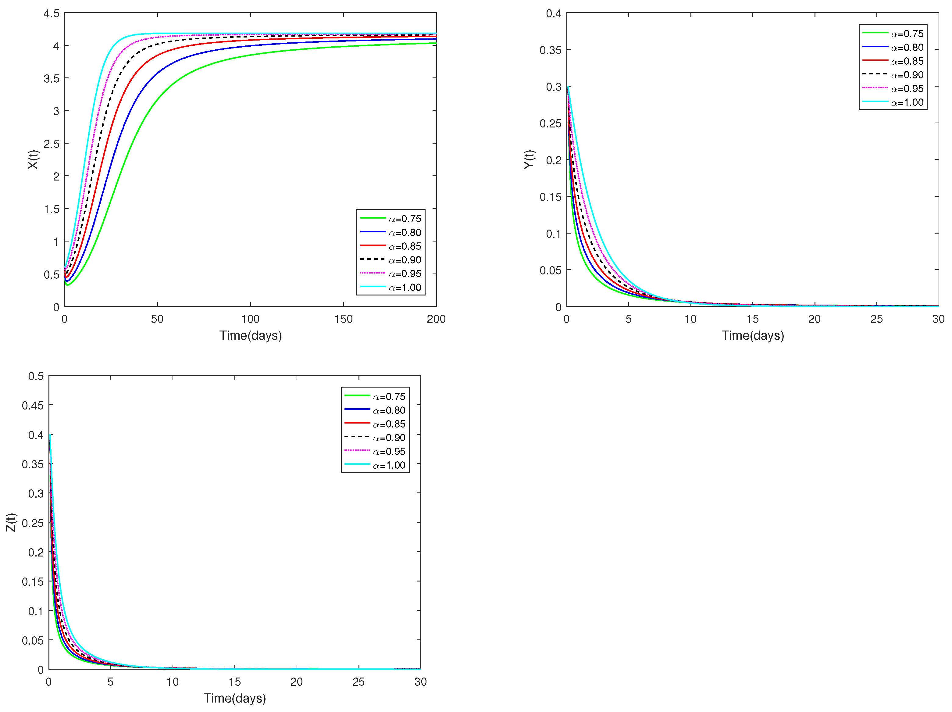
Example 1.

Fix the values of the following parameters:

$r=0.2$, $K=4.5$, $a=0.21$, $m=0.2$, $\mu =0.9$, $\gamma =0.4$, $d_1=0.02$, $d_2=0.1$, $d_3=1.6$, $d_4=0.1$, $\eta =0.7$, $q_1=0.2$ and $q_2=0.3$, $u_1=0.1$, $u_2=0.25$.

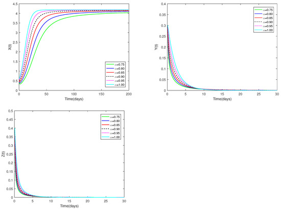
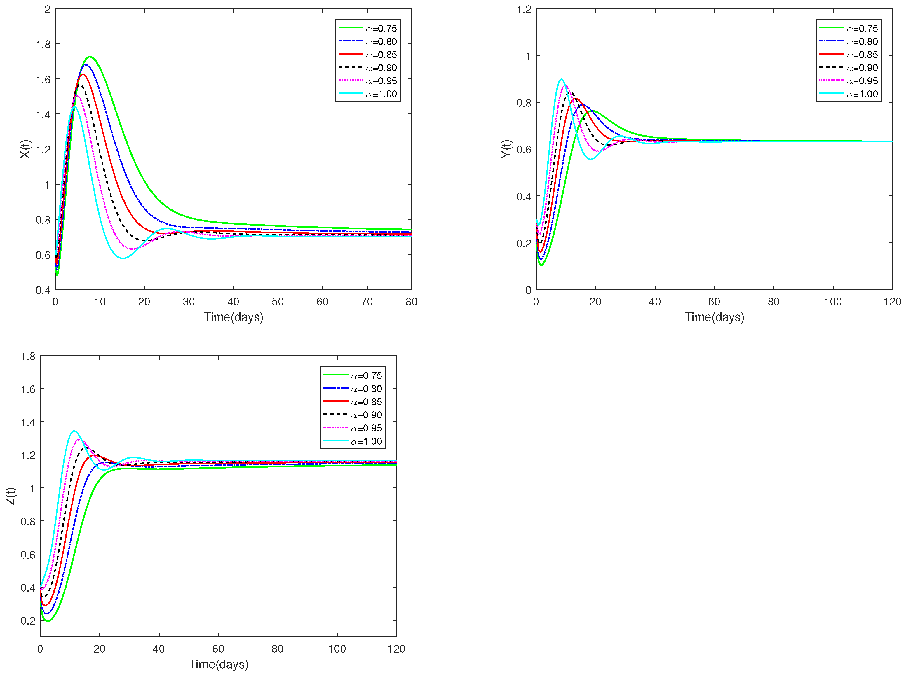
The initial value is designated as $Y_0=[0.6,0.3,0.4]$, and α have different values ($\alpha =0.75,0.80,0.85,0.90,0.95,1.00$). Figure 1 demonstrates that for any $\alpha \in [0.75,1]$, the predator-free equilibrium $E_1$ consistently exhibits asymptotic stable. Figure 1 clearly shows how the number of prey and predators changes when α changes from 0.75 to 1. This effect is obviously more specific than the integer order.

Example 2.

Fix the values of the following parameters:

$r=0.2$, $K=4.5$, $a=0.21$, $m=0.2$, $\mu =0.9$, $\gamma =0.4$, $d_1=0.02$, $d_2=0.1$, $d_3=1.6$, $d_4=0.1$, $\eta =0.7$, $q_1=0.2$ and $q_2=0.3$, $u_1=0.1$, $u_2=0.25$.

$Y_0=[0.3,0.2,0.2]$, $[0.6,0.3,0.4],[1.0,0.6,0.8]$, $[1.5,0.8,1.0],[1.8,1.0,1.2],[2.5,1.3,1.5]$ are used as the starting values, and α is set at $0.85$. Different starting values have no effect on the stability of the predator-free equilibrium $E_1$ of system (1), as Figure 2 shows.

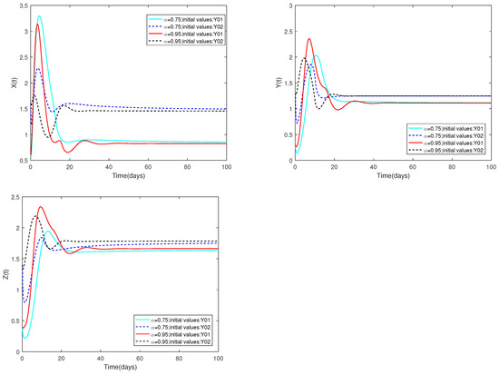
Example 3.

Fix the values of the following parameters: $r=1.1$, $K=3$, $a=0.71$, $m=0.2$, $\mu =0.9$, $\gamma =0.4$, $d_1=0.12$, $d_2=0.1$, $d_3=0.1$, $d_4=0.1$, $\eta =0.7$, $q_1=0.5$ and $q_2=0.5$, $u_1=0.515$, $u_2=0.515$.

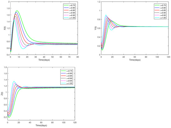
The initial value is designated as $Y_0=[0.6,0.3,0.4]$, and α have different values ($\alpha =0.75,0.80,0.85,0.90,0.95,1.00$). Figure 3 illustrates that when α is within the interval $[0.75,1]$, positive equilibrium $E_2$ demonstrates asymptotic stability. Figure 3 clearly shows how the number of prey and predators changes when α changes from 0.75 to 1. This effect is obviously more specific than the integer order.

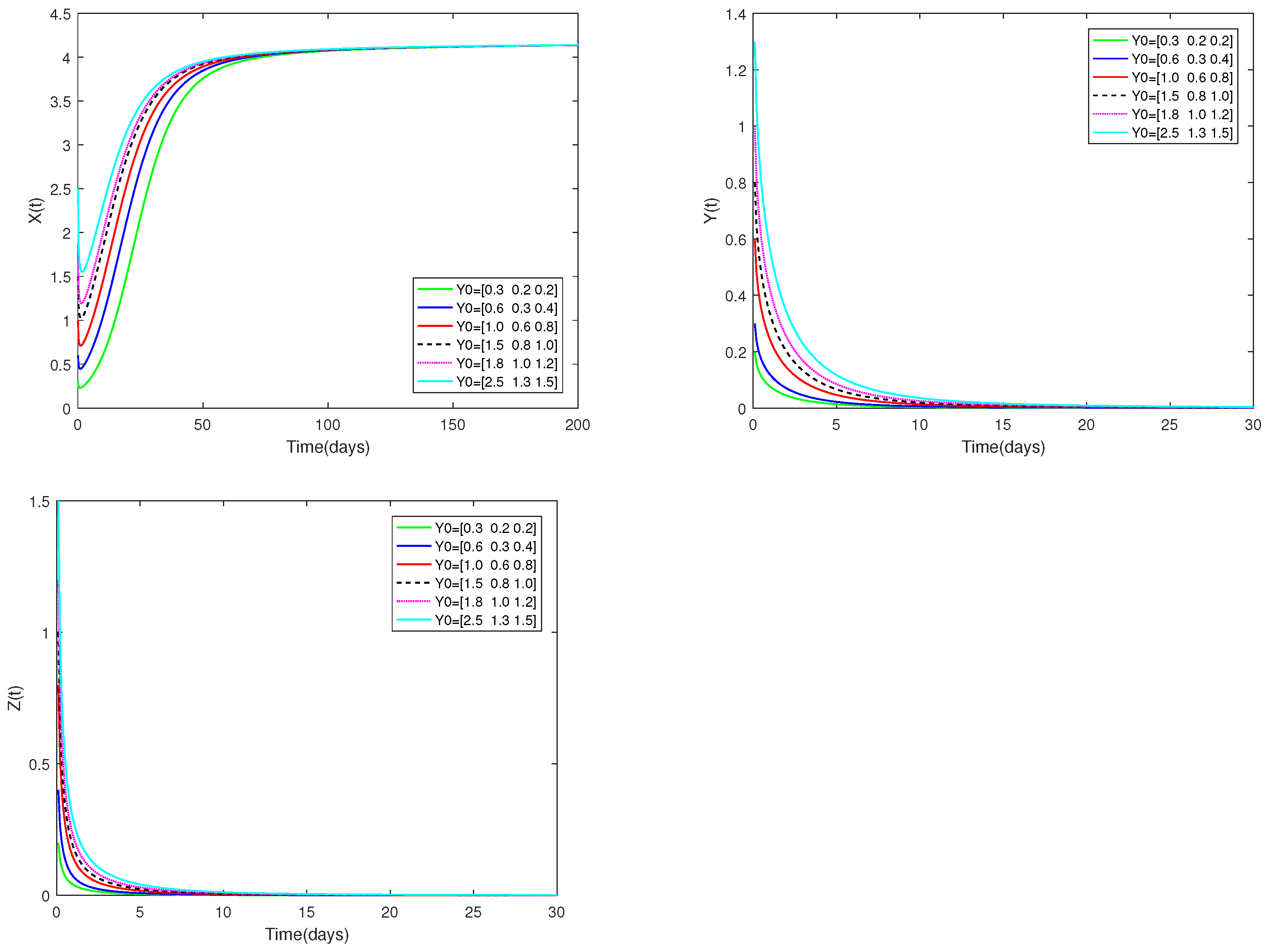
Example 4.

Fix the values of the following parameters: $r=1.1$, $K=3$, $a=0.71$, $m=0.2$, $\mu =0.9$, $\gamma =0.4$, $d_1=0.12$, $d_2=0.1$, $d_3=0.1$, $d_4=0.1$, $\eta =0.7$, $q_1=0.5$ and $q_2=0.5$, $u_1=0.515$, $u_2=0.515$.

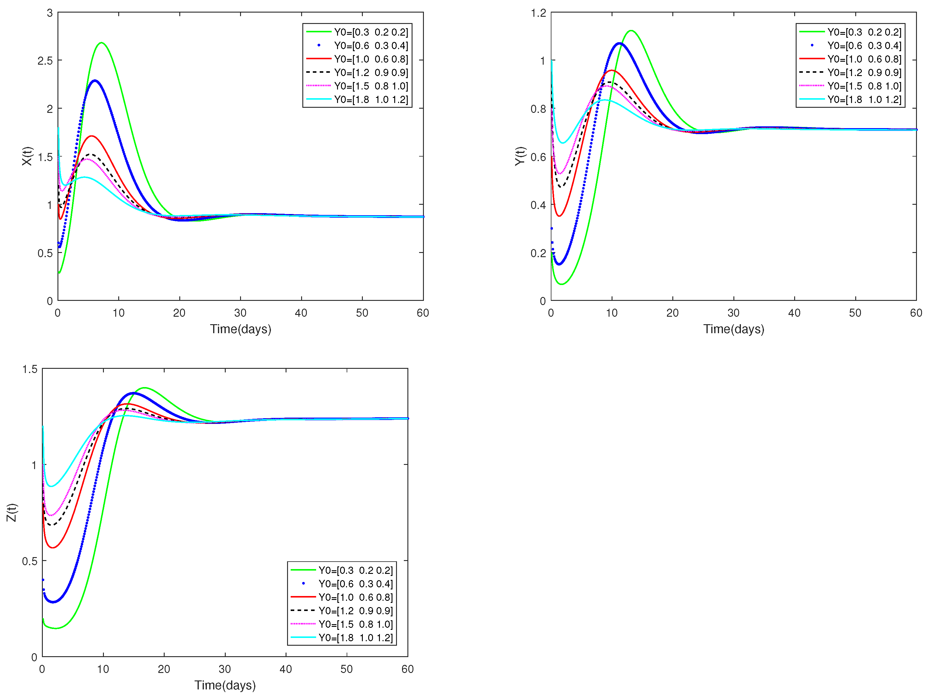
$Y_0=[0.3,0.2,0.2]$, $[0.6,0.3,0.4],[1.0,0.6,0.8]$, $[1.2,0.9,0.9],[1.5,0.8,1.0],[1.8,1.0,1.2]$ are used as the starting values, and α is set at $0.85$. As can be seen from Figure 4, the stability of the positive equilibrium $E_2$ of system (1) is not affected by various starting values.

Example 5.

Fix the values of the following parameters: $r=1.1$, $K=3$, $a=0.71$, $\mu =0.9$, $\gamma =0.4$, $d_1=0.12$, $d_2=0.1$, $d_3=0.1$, $d_4=0.1$, $\eta =0.7$, $q_1=0.2$ and $q_2=0.3$, $u_1=0.515$, $u_2=0.515$.

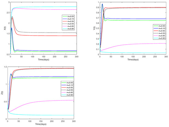
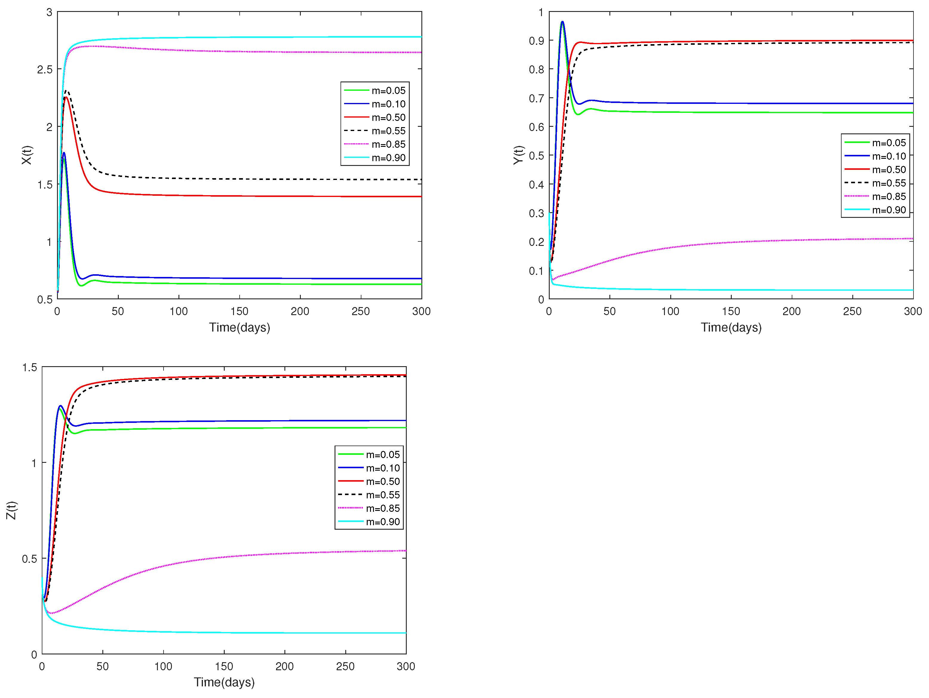
In Figure 5, the value of α and initial values are fixed to 0.85 and $Y_0=[0.6,0.3,0.4]$, and different values for m ($m=0.05$, 0.10, 0.50, 0.55, 0.85, 0.90) are taken, the objective is to examine how different m values affect system (1).

Example 6.

Fix the values of the following parameters: $r=1.1$, $K=3$, $a=0.71$, $m=0.2$, $\mu =0.9$, $\gamma =0.4$, $d_1=0.12$, $d_2=0.1$, $d_3=0.1$, $d_4=0.1$, $q_1=0.8$ and $q_2=0.3$, $u_1=0.515$, $u_2=0.515$.

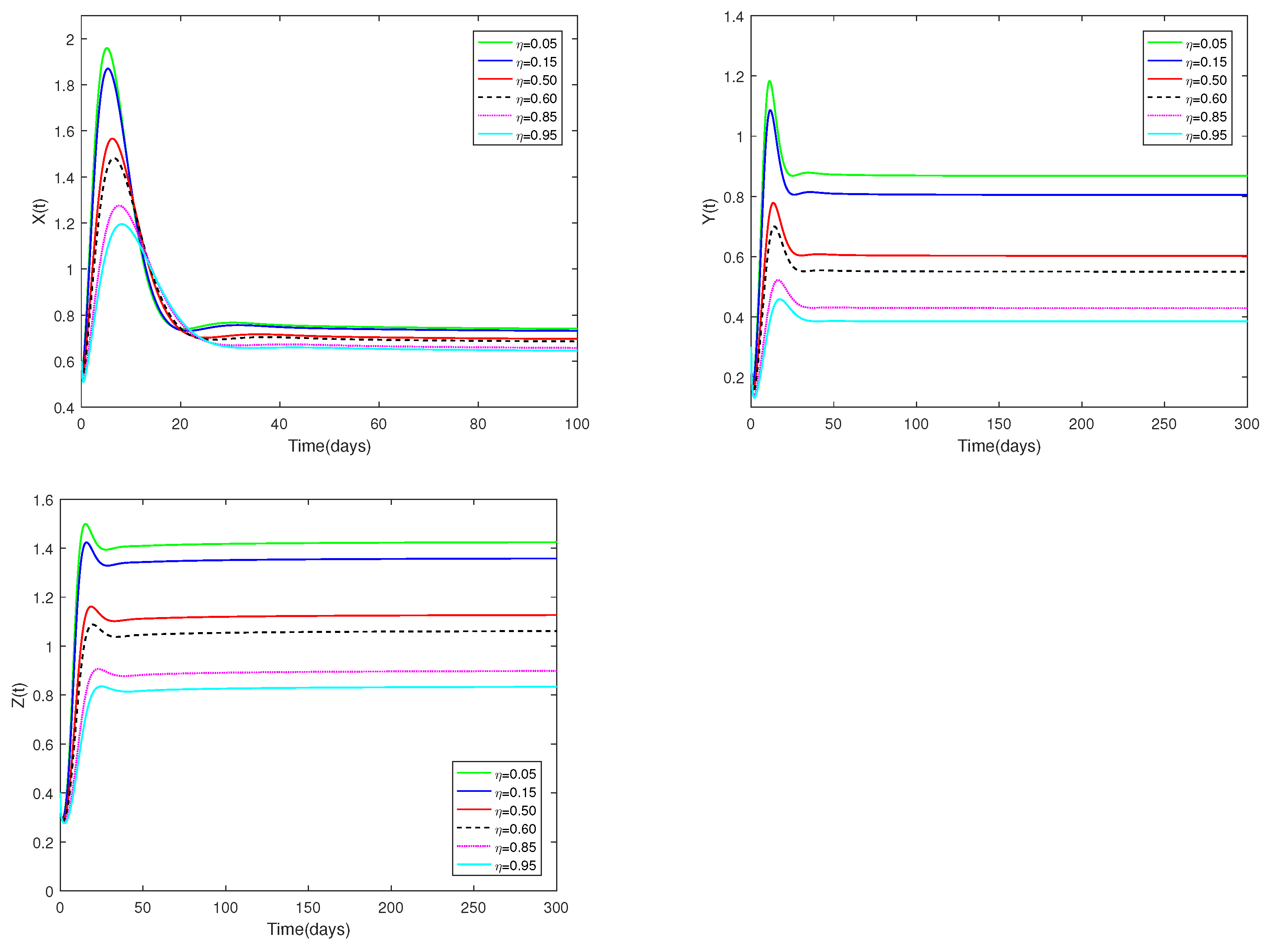
In Figure 6, the value of α and initial values are fixed to 0.85 and $Y_0=[0.6,0.3,0.4]$, and different values for η ($\eta =0.05$, 0.15, 0.50, 0.60, 0.85, 0.95) are taken, the objective is to analyze how different η values affect system (1).

Example 7.

Fix the values of the following parameters: $r=1.1$, $K=3$, $a=0.71$, $m=0.2$, $\mu =0.9$, $\gamma =0.4$, $d_1=0.12$, $d_2=0.1$, $d_3=0.1$, $d_4=0.1$, $\eta =0.7$ and $q_2=0.3$, $u_1=0.515$, $u_2=0.515$.

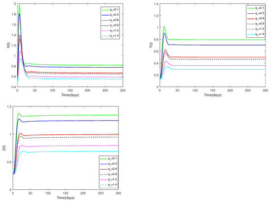
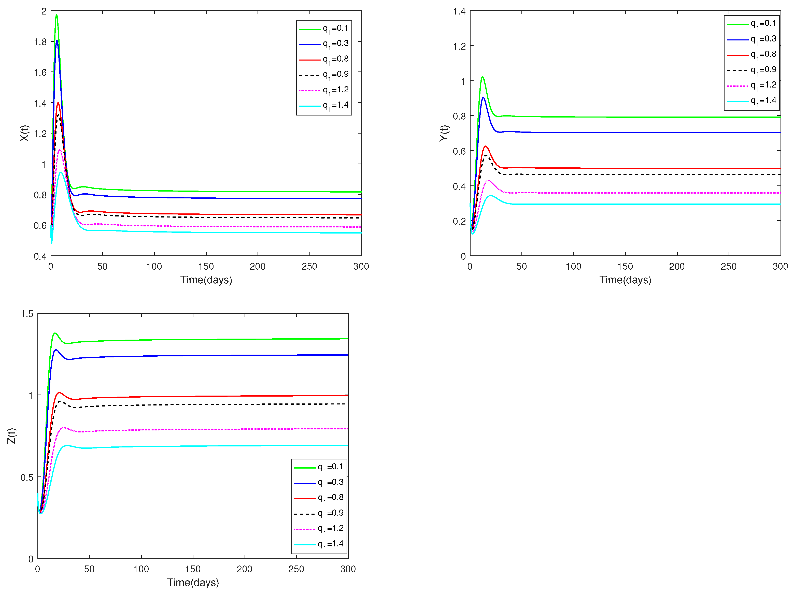
In Figure 7, the value of α and initial values are fixed to 0.85 and $Y_0=[0.6,0.3,0.4]$, and different values for $q_1$ ($q_1=0.1$, 0.3, 0.8, 0.9, 1.2, 1.4) are taken, the objective is to examine how different $q_1$ values affect system (1).

Example 8.

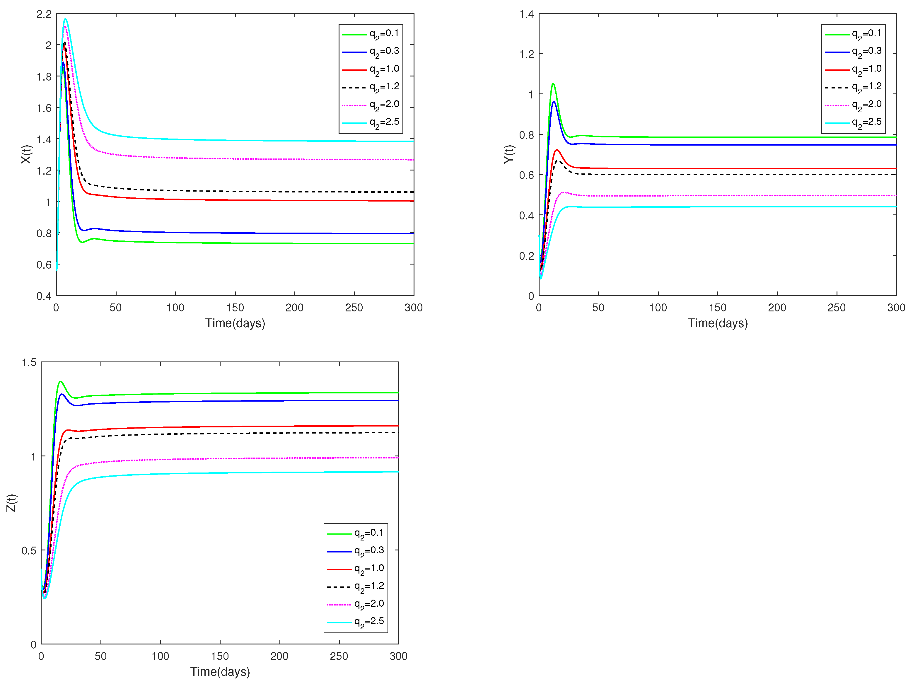
Fix the values of the following parameters: $r=1.1$, $K=3$, $a=0.71$, $m=0.2$, $\mu =0.9$, $\gamma =0.4$, $d_1=0.12$, $d_2=0.1$, $d_3=0.1$, $d_4=0.1$, $\eta =0.7$ and $q_1=0.3$, $u_1=0.515$, $u_2=0.515$.

In Figure 8, the value of α and initial values are fixed to 0.85 and $Y_0=[0.6,0.3,0.4]$, and different values for $q_2$ ($q_2=0.1$, 0.3, 1.0, 1.2, 2.0, 2.5) are taken, the objective is to analyze how different $q_2$ values affect system (1).

The following is a summary of the numerical simulation’s findings.

Remark 5.

(i) The predator-free equilibrium $E_1$ is shown to exist and to be stable in Figure 1 and Figure 2. Figure 3 and Figure 4 indicate that the co-existence equilibrium $E_2$ exists and the co-existence equilibrium $E_2$ is stable.

(ii) $E_1$ and $E_2$ are stable regardless of changes in α, as shown by Figure 1 and Figure 3. The value of α only affects the rate at which the equilibrium becomes stable.

(iii) Figure 2 and Figure 4 show that the stability of $E_1$ and $E_2$ is independent of the initial values, which is in line with Theorems 1, 2, 4 and 5. The initial values only can affect the rate at which the equilibrium becomes stable.

Remark 6.

(i) Figure 5 shows the sensitivity analysis of parameters m. It is evident that prey and predators are significantly impacted by the coefficient of prey refuge., however has no impact on the stability of the co-existence equilibrium $E_2$. While m is relatively large (close to 1), it indicates that the proportion of prey protected by the refuge is relatively large, and the prey population will remain unchanged after a sharp increase in a short period of time. In contrast, when m is relatively small (near 0), the number of prey increases and then decreases for a short period of time, and stays the same as the time approaches 50. This indicates that when the value of m is close to 1, it is conducive to the survival of the prey, but leads to a lower number of predators. But that doesn’t fit to predators. It is clear from the picture that both juvenile and adult predators are most abundant when $m=0.50,0.55$ (moderate).

(ii) Figure 6 show the sensitivity analysis of parameters η. It is evident that the amount of prey (young predator) that is available for harvesting has a big impact on both prey and predators, but it has no effect on how stable the coexistence equilibrium $E_2$ is. Regardless of whether η is large or small, the number of prey and predators increases first, then decreases, and finally stays stable. When η is relatively large (close to 1), it indicates that the proportion of prey and immature predator caught is relatively large. Naturally, when the value of η is relatively small (close to 0), it indicates that the proportion of captured prey and immature predators is small. Such a stark contrast suggests that a larger η leads to fewer immature predators and prey.

Remark 7.

(i) An analysis of the effects of parameters $q_1$ and $q_2$ on system (1) is displayed in Figure 7 and Figure 8.

(ii) The parameters $q_1$ and $q_2$ are shown to have a substantial impact on predators and prey, but they have no influence on the co-existence equilibrium $E_2$’s stability.

(iii) Regardless of whether $q_1$ and $q_2$ are large or small, the number of prey and predators increases first, then decreases, and finally stays stable. The number of prey and predators increase as $q_1$ decrease. The amount of predators decreases as $q_2$ grows, but the number of prey increases as $q_2$ increases.

5.2. Examples and Numerical Simulation Results for Optimal Control Problem

The values of parameters are obtained from [3,9].

Example 9.

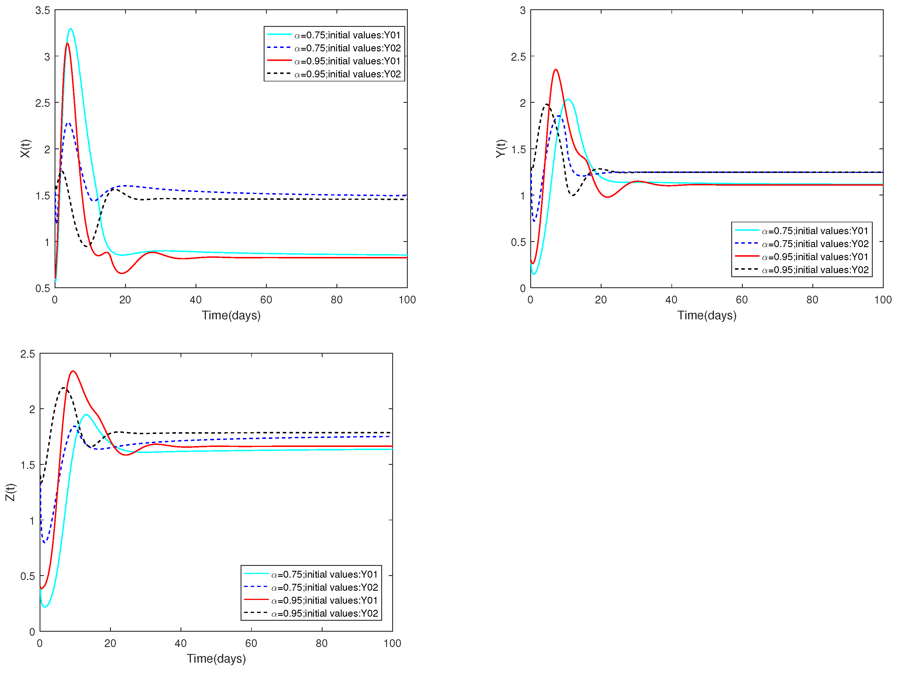
Fix the following parameter values: $r=1.5$, $K=4.5$, $a=0.71$, $m=0.20$, $\mu =0.9$, $\gamma =0.4$, $d_1=0.12$, $d_2=0.1$, $d_3=0.1$, $d_4=0.1$, $\eta =0.7$, $q_1=0.2$, $q_2=0.3$, $p_1=1.6$, $p_2=2.0$, $A_1=0.125$, $A_2=0.5$, $c_1=0.4$, $c_2=0.4$ and $\delta =0.01$.

$Y_{01}=[0.6,0.3,0.4,0,0,0,0,0],Y_{02}=[1.6,1.3,1.4,0,0,0,0,0]$ are used as the starting values, and α are set at $0.75$ and $0.95$.

Remark 8.

(i) Figure 9 illustrates that the initial values are identical, and altering the parameter α results in variations in the peak values of each state as well as differences in the rate of stabilization of system $(13)$.

(ii) The α value does not change, and the case for changing the initial is the same as above.

Example 10.

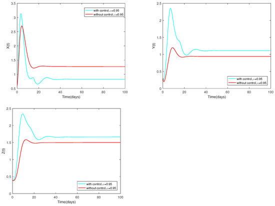
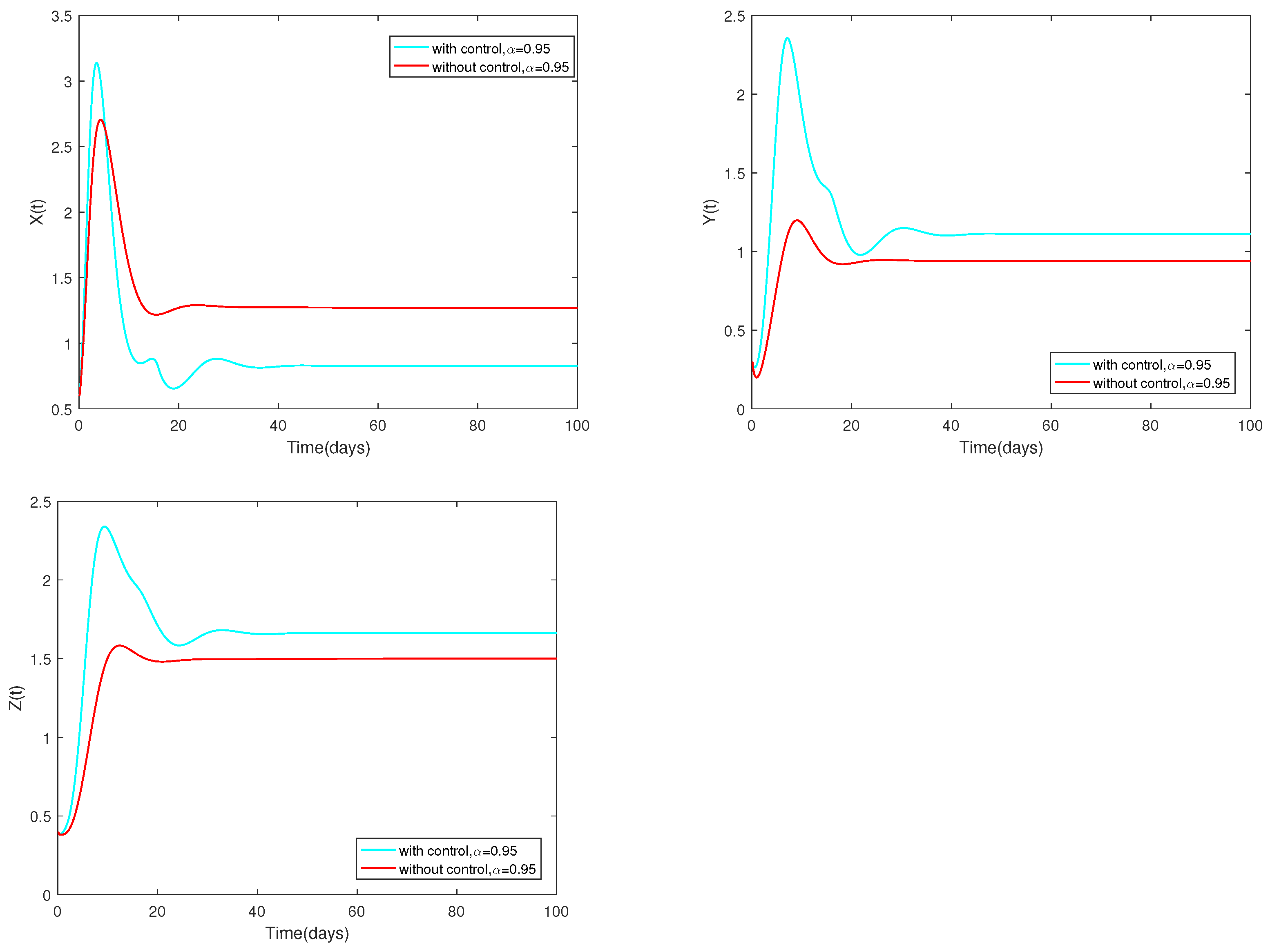
Fix the following parameter values: $r=1.5$, $K=4.5$, $a=0.71$, $m=0.20$, $\mu =0.9$, $\gamma =0.4$, $d_1=0.12$, $d_2=0.1$, $d_3=0.1$, $d_4=0.1$, $\eta =0.7$, $q_1=0.2$, $q_2=0.3$, $p_1=1.6$, $p_2=2.0$, $A_1=0.125$, $A_2=0.5$, $c_1=0.4$, $c_2=0.4$ and $\delta =0.01$.

The variable α is assigned to 0.95. The dynamic change of the system $(13)$ is depicted in Figure 10 either with an optimal ($u_1=u_1^{\ast }(t),u_2=u_2^{\ast }(t)$) or without control ($u_1=0,u_2=0$).

Remark 9.

(i) As can be seen from Figure 10, when optimal control exists, it will affect the amplitude and the stable state of system $(13)$.

(ii) Figure 10 also shows that with or without control, the system $(13)$ has an optimal solution, and the system $(13)$ can reach a stable state.

6. Discussions and Conclusions

6.1. Discussions

In this text, a fractional order fishery model with stage structure are established to study the effect of fractional derivative operators, prey refuge and protected areas. In the absence of control measures, we discuss whether equilibriums of the basic model are exist and are stable. Using Pontryagin’s maximum principle, the ideal solution for the enhanced model is determined.

System (1) yielded the following results from its qualitative analysis.

♡ As long as the initial value is positive, there is always a unique positive solution. Moreover, within this system, the set $\Gamma$ maintains positively invariant. This is a crucial conclusion from a biological standpoint.

♡ The co-existence equilibrium $E_2$ and predator-free equilibrium $E_1$ are shown to exist and be stable under the deduced necessary conditions.

The following is the conclusion drawn from the numerical simulation outcomes of system (1).

♡ Figure 1 and Figure 3 illustrate that the stability of equilibriums does not change when $\alpha$ changes. Only the rate at which the equilibriums become stable can be affected by the value of $\alpha$. Figure 2 and Figure 4 show that the stability of equilibriums is independent of the starting values. The initial values just can affect the speed towards the equilibriums.

Figure 1, Figure 2, Figure 3 and Figure 4 demonstrate that the beginning value is not significant and has no effect on stability. However, the value of $\alpha$ is important, and it will affect the speed at which the system tends to stabilization. And the fractional order is used to make the number changes of prey and predators more detailed and specific.

♡ From Figure 5, we can conclude that system (1) is sensitive to the parameter m. In other words, the number of prey and predators changes when m changes, but the stability of $E_2$ is not affected. When m is particularly large (close to 1), it is beneficial for the prey. So normally, when m is very small, it is good for the predator. However, Figure 5 shows that the predator population is larger when m is moderate ($m=0.50, 0.55$). This result reminds us that a moderate m will be more consistent with the sustainable development of the ecosystem.

♡ Figure 6 shows that increasing or decreasing $\eta$ does not change stability of $E_2$, but does change the number of prey and predator populations.

♡ Figure 7 and Figure 8 show the catchability co-efficients of prey and immature predator available for harvesting have a significant effect on prey and predators, however the interior equilibrium’s stability is not affected. Figure 7 and Figure 8 suggest that human beings can appropriately increase values of $q_1$ and $q_2$ to obtain more economic benefits on the premise of not destroying ecological sustainable development.

The following describes the qualitative and numerical outcomes of the optimal control issue.

♡ Applying the Pontryagin’s maximum principle, the optimal control solution formulas $u_1^{\ast }(t)$ and $u_2^{\ast }(t)$ are found.

♡ Figure 9 shows that when the initial value is fixed and $\alpha$ is changed, the stability of system (13) does not changes, only the peak values of prey and predators are affected. The same is true when $\alpha$ is fixed and the initial value is changed.

♡ Figure 10 shows that with or without control will not change the presence or absence of the optimal solution, but will cause the optimal solution of to take on various values. Figure 10 shows that when $\alpha$ is fixed, the presence of control measures would favor predator development.

6.2. Conclusions

A fractional model with refuge, reserve, and stage structure is examined in this work. It is demonstrated that the system is bounded, positive, and has a unique solution. Both the predator-free equilibrium $E_1$ and co-existence equilibrium $E_2$ exist in the system. We find the adequate circumstances under which $E_1$ and $E_2$ are locally stable. We demonstrate the globally asymptotically stable nature of the co-existence equilibrium $E_2$ using the Lozinskii measure. Using the effort used to harvest prey $u_1$ and effort used to harvest immature predator $u_2$ as controls yields the optimal solution that maximizes the economic benefit. Numerical simulations are used to explain how certain parameters affect the system. We can therefore conclude that the system’s stability is unaffected by the parameters $m,\eta ,q_1,q_2$. The fractional system will describe the system changes more precisely. The optimal solution can maximize the economic benefits of fishery institutions or fishermen without destroying the ecological balance.

References

- Liu, S.; Chen, L.; Agarwal, R. Recent progress on stage–structured population dynamics. Math. Comput. Model. 2002, 36, 1319–1360. [Google Scholar] [CrossRef]
- Swain, D.P.; Jonsen, I.D.; Simon, J.E.; Myers, R.A. Assessing threats to species at risk using stage-structured state–space models: Mortality trends in skate populations. Ecol. Appl. 2009, 19, 1347–1364. [Google Scholar] [CrossRef] [PubMed]
- Chakraborty, K.; Chakraborty, M.; Kar, T.K. Optimal control of harvest and bifurcation of a prey–predator model with stage structure. Appl. Math. Comput. 2011, 217, 8778–8792. [Google Scholar] [CrossRef]
- Chakraborty, K.; Jana, S.; Kar, T.K. Global dynamics and bifurcation in a stage structured prey–predator fishery model with harvesting. Appl. Math. Comput. 2012, 218, 9271–9290. [Google Scholar] [CrossRef]
- Holden, M.H.; Conrad, J.M. Optimal escapement in stage–structured fisheries with environmental stochasticity. Math. Biosci. 2015, 269, 76–85. [Google Scholar] [CrossRef] [PubMed]
- Lu, Y.; Pawelek, K.A.; Liu, S. A stage–structured predator–prey model with predation over juvenile prey. Appl. Math. Comput. 2017, 297, 115–130. [Google Scholar] [CrossRef]
- Mortoja, S.G.; Panja, P.; Mondal, S.K. Dynamics of a predator–prey model with stage–structure on both species and anti–predator behavior. Inform. Med. Unlocked 2018, 10, 50–57. [Google Scholar] [CrossRef]
- Zhao, X.; Zeng, Z. Stationary distribution of a stochastic predator–prey system with stage structure for prey. Physica A 2020, 545, 123318. [Google Scholar] [CrossRef]
- Mondal, N.; Paul, S.; Mahata, A.; ali Biswas, M.; Roy, B.; Alam, S. Study of dynamical behaviors of harvested stage–structured predator–prey fishery model with fear effect on prey under interval uncertainty. Franklin Open 2024, 6, 100060. [Google Scholar] [CrossRef]
- McNair, J.N. The effects of refuges on predator–prey interactions: A reconsideration. Theor. Popul. Biol. 1986, 29, 38–63. [Google Scholar] [CrossRef]
- Sih, A. Prey refuges and predator–prey stability. Theor. Popul. Biol. 1987, 31, 1–12. [Google Scholar] [CrossRef]
- Ruxton, G.D. Short term refuge use and stability of predator–prey models. Theor. Popul. Biol. 1995, 47, 1–17. [Google Scholar] [CrossRef]
- Křivan, V. Effects of optimal antipredator behavior of prey on predator–prey dynamics:the role of refuges. Theor. Popul. Biol. 1998, 53, 131–142. [Google Scholar] [CrossRef] [PubMed]
- Olivares, E.G.; Jiliberto, R.R. Dynamic consequences of prey refuges in a simple model system: More prey, fewer predators and enhanced stability. Ecol. Model. 2003, 166, 135–146. [Google Scholar] [CrossRef]
- Devi, S. Effects of prey refuge on a ratio–dependent predator–prey model with stage–structure of prey population. Appl. Math. Model. 2013, 37, 4337–4349. [Google Scholar] [CrossRef]
- Sharma, S.; Samanta, G.P. A Leslie–Gower predator–prey model with disease in prey incorporating a prey refuge. Chaos Solitons Fractals 2015, 70, 69–84. [Google Scholar] [CrossRef]
- Das, M.; Maiti, A.; Samanta, G.P. Stability analysis of a prey–predator fractional order model incorporating prey refuge. Ecol. Genet. Genom. 2018, 7–8, 33–46. [Google Scholar] [CrossRef]
- Zhang, H.; Cai, Y.; Fu, S.; Wang, W. Optimal control for the spread of infectious disease: The role of awareness programs by media and antiviral treatment. Appl. Math. Comput. 2019, 356, 328–337. [Google Scholar]
- Chakraborty, B.; Bairagi, N. Complexity in a prey–predator model with prey refuge and diffusion. Ecol. Complex. 2019, 37, 11–23. [Google Scholar] [CrossRef]
- Das, A.; Samanta, G.P. A prey–predator model with refuge for prey and additional food for predator in a fluctuating environment. Physica A 2020, 538, 122844. [Google Scholar] [CrossRef]
- Barman, D.; Roy, J.; Alrabaiah, H.; Panja, P.; Mondal, S.P.; Alam, S. Impact of predator incited fear and prey refuge in a fractional order prey predator model. Chaos Solitons Fractals 2021, 142, 110420. [Google Scholar] [CrossRef]
- Molla, H.; Sarwardi, S.; Smith, S.; Haque, M. Dynamics of adding variable prey refuge and an Allee effect to a predator–prey model. Alex. Eng. J. 2022, 61, 4175–4188. [Google Scholar] [CrossRef]
- Pandey, S.; Ghosh, U.; Das, D.; Chakraborty, S.; Sarkar, A. Rich dynamics of a delay–induced stage–structure prey-predator model with cooperative behavior in both species and the impact of prey refuge. Math. Comput. Simul. 2024, 216, 49–76. [Google Scholar] [CrossRef]
- Yang, P. Hopf bifurcation of age–structure prey–predator model with Holling type II functional response incorporating a prey refuge. Nonlinear Anal. Real World Appl. 2019, 49, 368–385. [Google Scholar] [CrossRef]
- Singh, A.; Sharma, V.S. Bifurcations and chaos control in a discrete–time prey–predator model with Holling type II functional response and prey refuge. J. Comput. Appl. Math. 2023, 418, 114666. [Google Scholar] [CrossRef]
- Xiang, C.; Huang, J.; Wang, H. Bifurcations in Holling–Tanner model with generalist predator and prey refuge. J. Differ. Equ. 2023, 343, 495–529. [Google Scholar] [CrossRef]
- Javadi, M.; Nyamoradi, N. Dynamic analysis of a fractional order prey–predator interaction with harvesting. Appl. Math. Model. 2013, 37, 8946–8956. [Google Scholar] [CrossRef]
- Rivero, M.; Trujillo, J.J.; Vazquez, L.; Velasco, M.P. Fractional dynamics of populations. Appl. Math. Comput. 2011, 218, 1089–1095. [Google Scholar] [CrossRef]
- Ghaziani, P.K.; Alidousti, J.; Eshkaftaki, A.B. Stability and dynamics of a fractional order Leslie–Gower prey–predator model. Appl. Math. Comput. 2016, 40, 2075–2086. [Google Scholar]
- Mansal, F.; Sene, N. Analysis of fractional fishery model with reserve area in the context of time–fractional order derivative. Chaos Solitons Fractals 2020, 140, 110200. [Google Scholar] [CrossRef]
- Balci, E. Predation fear and its carry–over effect in a fractional order prey-predator model with prey refuge. Chaos Solitons Fractals 2023, 175, 114016. [Google Scholar] [CrossRef]
- Chu, C.; Liu, W.; Lv, G.; Moussaoui, A.; Auger, P. Optimal harvest for predator–prey fishery models with variable price and marine protected area. Commun. Nonlinear Sci. Numer. Simul. 2024, 134, 107992. [Google Scholar] [CrossRef]
- Liu, X.; Huang, Q. Analysis of optimal harvesting of a predator–prey model with Holling type IV functional response. Ecol. Complex. 2020, 42, 1008165. [Google Scholar] [CrossRef]
- Ibrahim, M. Optimal harvesting of a predator–prey system with marine reserve. Sci. Afr. 2021, 14, e01048. [Google Scholar] [CrossRef]
- Haukkanen, P.; Tossavainen, T. A generalization of Descartes’ rule of signs and fundamental theorem of algebra. Appl. Math. Comput. 2011, 218, 1203–1207. [Google Scholar] [CrossRef]
- Yıldız, T.A.; Arshad, S.; Baleanu, D. New observations on optimal cancer treatments for a fractional tumor growth model with and without singular kernel. Chaos Solitons Fractals 2018, 117, 226–239. [Google Scholar] [CrossRef]
- Ahmed, E.; El-Sayed, A.; El-Saka, H. On some Routh–Hurwitz conditions for fractional order differential equations and their applications in Lorenz, Rssler, Chua and Chen systems. Phys. Lett. A 2006, 358, 1–4. [Google Scholar] [CrossRef]
- Pinto, C.; Carvalho, A. A latency fractional order model for HIV dynamics. J. Comput. Appl. Math. 2017, 312, 240–256. [Google Scholar] [CrossRef]
- Li, Y.; Muldowney, J.S. On Bendixson’s criterion. J. Differ. Equ. 1993, 106, 709–726. [Google Scholar] [CrossRef]
- Burler, G.; Freedman, H.I.; Waltman, P. Uniformly persistent systems. Proc. Am. Math. Soc. 1986, 96, 425–430. [Google Scholar]
- Buonomo, B.; D’Onofrio, A.; Lacitiguola, D. Global stability of an SIR epidemic model with information dependent vaccination. Math. Biosci. 2008, 216, 9–16. [Google Scholar] [CrossRef] [PubMed]
- Martin, R.H., Jr. Logarithnic norms and projections applied to linear differential systems. J. Math. Anal. Appl. 1974, 45, 240–256. [Google Scholar] [CrossRef]
- Shi, R.; Zhang, Y. Dynamic analysis and optimal control of a fractional order HIV/HTLV co–infection model with HIV–specific antibody immune response. AIMS Math. 2024, 9, 9455–9493. [Google Scholar] [CrossRef]
- Kamien, M.I.; Schwartz, N.L. Dynamic Optimization: The Calculus of Variations and Optimal Control in Economics and Management; Elsevier: New York, NY, USA, 1991. [Google Scholar]
- Ahmed, E.; El-Sayed, A.M.A.; El-Saka, H.A.A. Equilibrium points, stability and numerical solutions of fractional–order predator–prey and rabies models. J. Math. Anal. Appl. 2007, 325, 542–553. [Google Scholar] [CrossRef]
- El-Sayed, A.M.A.; El-Mesiry, E.M.; El-Saka, H.A.A. Numerical solution for multi-term fractional (arbitrary) orders differential equations. Comput. Appl. Math. 2004, 23, 33–54. [Google Scholar] [CrossRef]
Disclaimer/Publisher’s Note: The statements, opinions and data contained in all publications are solely those of the individual author(s) and contributor(s) and not of MDPI and/or the editor(s). MDPI and/or the editor(s) disclaim responsibility for any injury to people or property resulting from any ideas, methods, instructions or products referred to in the content. |
© 2024 by the authors. Licensee MDPI, Basel, Switzerland. This article is an open access article distributed under the terms and conditions of the Creative Commons Attribution (CC BY) license (https://creativecommons.org/licenses/by/4.0/).