Pretest Estimation for the Common Mean of Several Normal Distributions: In Meta-Analysis Context

Abstract

The estimation of unknown quantities from multiple independent yet non-homogeneous samples has garnered increasing attention in various fields over the past decade. This interest is evidenced by the wide range of applications discussed in recent literature. In this study, we propose a preliminary test estimator for the common mean $\left(\mu \right)$ with unknown and unequal variances. When there exists prior information regarding the population mean with consideration that $\mu$ might be equal to the reference value for the population mean, a hypothesis test can be conducted: $H_0:\mu ={\mu }_0$ versus $H_1:\mu \ne {\mu }_0$. The initial sample is used to test $H_0$, and if $H_0$ is not rejected, we become more confident in using our prior information (after the test) to estimate $\mu$. However, if $H_0$ is rejected, the prior information is discarded. Our simulations indicate that the proposed preliminary test estimator significantly decreases the mean squared error (MSE) values compared to unbiased estimators such as the Garybill-Deal (GD) estimator, particularly when $\mu$ closely aligns with the hypothesized mean (${\mu }_0$). Furthermore, our analysis indicates that the proposed test estimator outperforms the existing method, particularly in cases with minimal sample sizes. We advocate for its adoption to improve the accuracy of common mean estimation. Our findings suggest that through careful application to real meta-analyses, the proposed test estimator shows promising potential.

1. Introduction

As medical knowledge continues to expand rapidly, healthcare providers face significant challenges in thoroughly evaluating and analyzing the necessary data to make well-informed decisions [1,2,3]. The complexity of these challenges is further heightened by the variety of findings, presented in different studies, which are sometimes conflicting. Meta-analysis, along with research synthesis or integration, has become an effective tool for addressing these issues. This method achieves its objective by applying rigorous statistical techniques to aggregate the results from multiple individual studies, thereby combining their findings [2,4]. Additionally, meta-analysis has gained widespread attention across numerous scientific fields, such as education, social sciences, and medicine. For example, in education has been used to consolidate research on the effectiveness of coaching in improving Scholastic Aptitude Test (SAT) scores in both verbal and mathematical sections [5]. In social sciences, it has been used to synthesize studies on gender differences in quantitative, verbal, and visual-spatial abilities [6]. In healthcare, meta-analysis has been particularly valuable during the COVID-19 pandemic, enhancing our understanding of the virus and informing public health strategies [7,8].

The challenge of combining two or more unbiased estimators is a common issue in applied statistics, with significant implications across various fields. A notable example of this problem occurred when Meier [9] was tasked with making inferences about the mean albumin level in plasma protein in human subjects using data from four separate experiments. Similarly, Eberhardt et al. [10] faced a scenario where they needed to draw conclusions about the mean selenium content in non-fat milk powder by integrating results from four different methods across four experiments.

Most of the early research on drawing inferences about the common mean $\left(\mu \right)$ focuses on point estimation and theoretical decision rules regarding $\mu$. Graybill and Deal were the first among a few researchers to research about estimating $\mu$ [11]. Since then, numerous works have been building upon and expanding upon their initial work [12,13,14,15,16,17,18], along with the related references. Conversely, Meier [9] developed a method for estimating the confidence interval for $\mu$. In addition, refs. [19,20] have devised approximate confidence intervals. The properties of such estimators have accumulated substantial attention in the literature. Sinha et al. [2] derived an unbiased estimator of the variance for the Graybill-Deal estimator, and Krishnamoorthy and Moore [21] considered this in the prediction problem of linear regression.

In some cases, researchers find situations where prior information $\left({\theta }_0\right)$ on the mean population is available, whether through pre-test information or historical data. Pretest or preliminary tests or shrinkage estimators involve the concept of leveraging preliminary information to improve parameter estimation accuracy. These estimators work with the idea of borrowing strength from both sample data and pre-test information, resulting in higher efficiency and reliability than traditional estimators. Bancroft [22] and Stein [23] introduced and extensively examined the preliminary test shrinkage estimator. Their method has influenced numerous advancements and applications in statistics and has established a basis for the use of shrinkage estimators in contemporary statistical practice [24,25,26]. Thompson [27] proposed a shrinkage technique given as

$$\omega =q{\theta }_0+(1-q)\theta ,$$

(1)

where $q=0$ (accept $H_0$), $q=1$ (reject $H_0$) and ${\theta }_0$ as prior guess. This was aimed at improving the current estimator of a parameter $\theta$ to estimate the mean, thereby reducing the mean square error (MSE) of the uniform minimum-variance unbiased estimator (UMVUE) for the population mean. It has been observed that the shrinkage estimator performs better than the conventional estimator when the assumed value of q aligns closely with the prior guess. Consequently, instead of treating q as a constant value in the shrinkage estimator, it is advisable to regard it as a weight ranging between 0 and 1 [27]. In this context, q can be viewed as a continuous function dependent on certain pertinent statistics, anticipating that its value will decrease consistently as the deviation $(\theta -{\theta }_0)$ from a reference value increases.

This preliminary test has been widely used in statistics [24,25,26]. Khan et al. [24] deployed a preliminary test for estimating the mean of a univariate normal population with an unknown variance. Shih et al. [25] proposed a class of general pretest estimators for the univariate normal mean which included numerous existing estimators, such as pretest, shrinkage, Bayes, and empirical Bayes estimators. In the context of meta-analysis, Taketomi et al. [26] proposed simultaneous estimation of individual means using the James–Stein shrinkage estimators, which improved upon individual studies’ estimators. Literature has observed that when prior information is available, shrinkage estimators for parameters of various distributions tend to outperform standard estimators in terms of MSE, especially when the estimated value is close to the true value [22,27,28].

The use of prior information in estimating the common mean has several significant advantages. For example, it allows researchers to leverage significant past knowledge, which could be from historical data, expert opinion, or preliminary investigations, improving the accuracy of the estimation process. Secondly, they tend to strike a compromise between bias and variance, resulting in estimates that are both unbiased and more efficient than traditional estimators, particularly in circumstances with small sample sizes. However, there are limited research studies on point estimation of $\mu$ proposing preliminary test-based estimators. It is therefore, in this study we propose a preliminary test estimator for the common mean with unknown and unequal variances. In order to find the ideal estimator, the properties of the proposed preliminary test estimator will be examined, which includes its theoretical basis and performance-based criteria such as bias and MSE.

2. Background

To define the current problem, we assume there are k independent normal populations with a common mean $\left(\mu \right)$, but with unknown and potentially unequal variances ${\sigma }_1^2,\dots ,{\sigma }_k^2>0$. We assume we have independent and identically distributed ($i.i.d$) observations $X_{i1},\dots ,X_{i{n}_i}$ from $N(\mu ,{\sigma }_i^2)$, $i=1,2,\cdots ,k$ and we define ${\overline{X}}_i$ and $S_i^2$ as

$$\begin{array}{ccc}\hfill {\overline{X}}_i& =& \sum _{j=1}^{n_i}{\displaystyle \frac{X_{ij}}{n_i}},\hfill \end{array}$$

(2)

$$\begin{array}{ccc}\hfill S_i^2& =& \sum _{j=1}^{n_i}{(X_{ij}-{\overline{X}}_i)}^2/(n_i-1),\hfill \end{array}$$

(3)

where ${\overline{X}}_i\sim N(\mu ,{\sigma }_i^2/n_i)$, $(n_i-1)S_i^2\sim {\sigma }_i^2{\chi }_{n_i-1}^2$. Note that these statistics $\{{\overline{X}}_i,S_i^2,i=1,2\}$ are all mutually independent. Again, it can be noted that $\{{\overline{X}}_1,S_1^2,{\overline{X}}_2,S_2^2,\cdots ,{\overline{X}}_k,S_k^2\}$ are minimal sufficient statistics for $(\mu ,{\sigma }_1^2,{\sigma }_2^2,\cdots ,{\sigma }_k^2)$ but not complete [29]. As a result, one cannot get the uniformly minimum variance unbiased estimator (UMVUE) if it exists using the standard Rao-Blackwell theorem on an unbiased estimator for estimating $\mu$. For the case of k when the population variances are fully known, $\mu$ can be readily estimated as

$$\begin{array}{ccc}\hfill \widehat{\mu }& =& \left(\sum _{i=1}^k{\displaystyle \frac{n_i}{{\sigma }_i^2}}{\overline{X}}_i\right)/\left(\sum _{i=1}^k{\displaystyle \frac{n_i}{{\sigma }_i^2}}\right),\hfill \end{array}$$

(4)

$$\begin{array}{ccc}\hfill \mathrm{Var}\left(\widehat{\mu }\right)& =& {\displaystyle \frac{1}{{\sum }_{i=1}^k\left(n_i/{\sigma }_i^2\right)}}.\hfill \end{array}$$

(5)

This estimator, $\widehat{\mu }$, is the UMVUE, the best linear unbiased estimator (BLUE), and the maximum likelihood estimator (MLE). In the context of our current problem, where the population variances are unknown and possibly unequal, the most appealing unbiased estimator for $\mu$ is the Graybill-Deal (GD) estimator [11], which is

$$\begin{array}{cc}\hfill {\widehat{\mu }}_{GD}& =\left(\sum _{i=1}^k{\displaystyle \frac{n_i}{S_i^2}}{\overline{X}}_i\right)/\left(\sum _{i=1}^k{\displaystyle \frac{n_i}{S_i^2}}\right),\hfill \end{array}$$

(6)

$$\begin{array}{cc}\hfill \mathrm{Var}\left({\widehat{\mu }}_{GD}\right)& =E\left[\sum _{i=1}^k\left({\displaystyle \frac{n_i{\sigma }_i^2}{S_i^4}}\right)/{\left(\sum _{i=1}^k{\displaystyle \frac{n_i}{S_i^2}}\right)}^2\right].\hfill \end{array}$$

(7)

In the case of two samples, GD [11] first demonstrated that an unbiased estimator ${\widehat{\mu }}_{GD}$ in Equation (6) has a lower variance compared to either sample mean, provided that both sample sizes exceed 10.

Khatri and Shah [30] proposed an exact variance formula for ${\widehat{\mu }}_{GD}$ which is complex and not easily applied. To tackle this inference issue, Meier [9] derived a first-order approximation of the variance of ${\widehat{\mu }}_{GD}$, given by

$$\begin{array}{cc}\hfill Var\left({\widehat{\mu }}_{GD}\right)& ={\left[\sum _{i=1}^k{\displaystyle \frac{n_i}{{\sigma }_i^2}}\right]}^{-1}\left[1+2\sum _{i=1}^k{\displaystyle \frac{1}{n_i-1}}{c}_i\left(1-c_i\right)+O\left(\sum _{i=1}^k{\displaystyle \frac{1}{{\left(n_i-1\right)}^2}}\right)\right],\hfill \end{array}$$

where $c_i={\displaystyle \frac{n_i/{\sigma }_i^2}{{\sum }_{j=1}^k{n}_j/{\sigma }_j^2}}$.

A few years later, Sinha [31] developed an unbiased estimator for the variance of $\widehat{\mu }$ that takes the form of a convergent series. A first-order approximation of this estimator is

$$\begin{array}{c}\hfill {\widehat{Var}}_{\left(1\right)}\left({\widehat{\mu }}_{GD}\right)={\displaystyle \frac{1}{{\sum }_{i=1}^k{n}_i/s_i^2}}\left[1+\sum _{i=1}^k{\displaystyle \frac{4}{n_i+1}}\left({\displaystyle \frac{n_i/s_i^2}{{\sum }_{j=1}^k{n}_j/s_j^2}}-{\displaystyle \frac{n_i^2/s_i^4}{{\left({\sum }_{j=1}^k{n}_j/s_j^2\right)}^2}}\right)\right].\end{array}$$

The above estimator is comparable to Meier’s [9] approximate estimator, defined as

$$\begin{array}{c}\hfill {\widehat{Var}}_{\left(2\right)}\left({\widehat{\mu }}_{GD}\right)={\displaystyle \frac{1}{{\sum }_{i=1}^k{n}_i/s_i^2}}\left[1+\sum _{i=1}^k{\displaystyle \frac{4}{n_i-1}}\left({\displaystyle \frac{n_i/s_i^2}{{\sum }_{j=1}^k{n}_j/s_j^2}}-{\displaystyle \frac{n_i^2/s_i^4}{{\left({\sum }_{j=1}^k{n}_j/s_j^2\right)}^2}}\right)\right].\end{array}$$

The “classical” meta-analysis variance estimator, ${\widehat{Var}}_{\left(3\right)}$ is given as

$$\begin{array}{c}\hfill {\widehat{Var}}_{\left(3\right)}\left({\widehat{\mu }}_{GD}\right)={\displaystyle \frac{1}{{\sum }_{i=1}^k{n}_i/s_i^2}}.\end{array}$$

Approximate variance estimator proposed by Hartung [32], ${\widehat{Var}}_{\left(4\right)}$ is given as

$$\begin{array}{c}\hfill {\widehat{Var}}_{\left(4\right)}\left({\widehat{\mu }}_{GD}\right)={\displaystyle \frac{1}{k-1}}\sum _{i=1}^k{\displaystyle \frac{n_i/s_i^2}{{\sum }_{j=1}^k{n}_j/s_j^2}}{\left({\overline{X}}_i-{\widehat{\mu }}_{GD}\right)}^2.\end{array}$$

3. Proposed Preliminary Test Estimator

It is reasonable to test a null hypothesis when uncertain non-sample prior information is available. A preliminary test estimator is a two-step process that estimates a key parameter using the results of a preliminary test. To estimate $\mu$, we consider the hypothesis

$$H_0:\mu ={\mu }_{0}vs.H_1:\mu \ne {\mu }_0.$$

(8)

Our proposed preliminary test estimate for $\mu$ is as follows:

$${\widehat{\mu }}_{PT}=\left\{\begin{array}{cc}{\mu }_0\hfill & ,\mathrm{if}{H}_0\mathrm{is}\mathrm{accepted}\hfill \\ {\widehat{\mu }}_{GD}=\left(\sum _{i=1}^k{\displaystyle \frac{n_i}{s_i^2}}{\overline{X}}_i\right)/\left(\sum _{i=1}^k{\displaystyle \frac{n_i}{s_i^2}}\right)\hfill & ,\mathrm{if}{H}_0\mathrm{is}\mathrm{rejected}\hfill \end{array}\right.$$

(9)

where ${\widehat{\mu }}_{GD}$ is unbiased estimator of $\mu$. Shih et al. [25] defined $a:\mathbb{R}\mapsto [0,1]$ be a test function with $a=0\left(\mathrm{accept}{H}_0\right)$, $a=1\left(\mathrm{reject}{H}_0\right)$, and $0<a<1\left(\mathrm{reject}{H}_0\mathrm{with}\mathrm{probability}a\right)$. For $0\le {\alpha }_1\le {\alpha }_2\le 1$, then randomized test is defined as

$$a\left(\mathbf{X}\right)=\left\{\begin{array}{cc}1\hfill & ,\mathrm{if}|t_{obs}| >t_{{\alpha }_1/2,n-1},\hfill \\ q\left(\mathbf{X}\right)\hfill & ,\mathrm{if}{t}_{{\alpha }_2/2,n-1}<\left|t_{obs}\right|\le t_{{\alpha }_1/2,n-1},\hfill \\ 0\hfill & ,\mathrm{if}|t_{obs}| \le t_{{\alpha }_2/2,n-1}.\hfill \end{array}\right.$$

The rejection or failure to reject $H_0$ will be based on the t statistic. A standard notation for a t statistic based on a sample of size n is $t_{obs}=\sqrt{n}\left(\overline{x}-{\mu }_0\right)/s$. We can refer to this t computed from a specific set of data as the observed value of our test statistic, and reject $H_0$ when $|t_{obs}| >t_{\alpha /2,\nu }$, where $\nu$ is $n-1$ degrees of freedom and $\alpha$ is Type-I error level. A test for $H_0$ based on a p-value on the other hand is based on $P_{obs}=P\left[\right|t_{\nu }| > |t_{obs}\left|\right]$, and we reject $H_0$ at level $\alpha$ if $P_{obs}<\alpha$. We let $t_{0,\nu }\equiv \infty$ as usual. Then $t_{\nu }$ stands for the central t variable with $\nu$ degrees of freedom, and $t_{\alpha /2,\nu }$ stands for the upper $\alpha /2$ percentile of $t_{\nu }$. The general preliminary test estimator [33] can be defined as

$${\widehat{\mu }}_{GPT}=a\left(\mathbf{X}\right){\widehat{\mu }}_{GD}+[1-a\left(\mathbf{X}\right)]{\mu }_0.$$

The estimator can also be written as

$$\begin{array}{ccc}\hfill {\widehat{\mu }}_{GPT}& =& {\mu }_0+({\widehat{\mu }}_{GD}-{\mu }_0)\mathbf{I}\left(\right|t_{obs}| >t_{{\alpha }_1/2,n-1})+\hfill \\ & & q\left(\mathbf{X}\right)\mathbf{I}(t_{{\alpha }_2/2,n-1}<|t_{obs}|\le t_{{\alpha }_1/2,n-1}).\hfill \end{array}$$

(10)

In this study, we focus only on the case where ${\alpha }_1={\alpha }_2=\alpha$. We can define our proposed preliminary test estimator with unknown variance as

$${\widehat{\mu }}_{PT}={\mu }_0+({\widehat{\mu }}_{GD}-{\mu }_0)\mathbf{I}\left(\right|t_{ran}| >t_{\alpha /2,n-1}),$$

(11)

where $\mathbf{I}(·)$ is the indicator function defined as $\mathbf{I}\left(A\right)=1$ if A is true and $\mathbf{I}\left(A\right)=0$ if A is false. A random p-value which has a $Uniform(0,1)$ distribution under $H_0$ is defined as $P_{ran}=P\left[\right|t_{\nu }| > |t_{ran}\left|\right]$, where $t_{ran}=\sqrt{n}\left(\overline{X}-{\mu }_0\right)/s$. Most suggested tests for $H_0$ are based on $P_{obs}$ and $t_{obs}$ values. To simplify the notation, we will denote $P_{obs}$ by small p and $P_{ran}$ by large P. In our context, we have independent t statistics, $t_1,\dots ,t_k$, and also independent p-values, $P_1,\dots ,P_k$. In the following, we suggest various test procedures for testing $\mu ={\mu }_0$ based on suitable combinations of $t_i^{\prime }s$ and $P_i^{\prime }s$ [34]. Depending on the test procedure we use, the rejection set A will be defined and used to compute the Bias and MSE of the preliminary test estimator of the common mean $\mu$.

3.1. P-Value Based Exact Tests

Suppose $P_{\left(1\right)},\cdots ,P_{\left(k\right)}$ are independent p-values obtained from k continuous distributions of test statistics, then when individual hypothesis $H_{0i}$ is true, $P_i$ is uniformly distributed over the interval $\left[0,1\right]$. Testing the joint null hypothesis $H_0:\mu ={\mu }_0$ versus $H_1:\mu \ne {\mu }_0$. Five p-value-based exact tests based on $t_{obs}$ and p-value from k independent studies as available in the literature are listed below.

3.1.1. Tippett’s Test

Suppose $P_{\left(1\right)},\cdots ,P_{\left(k\right)}$ are independent and ordered p-values. Then $H_0$ is rejected if $P_{\left(1\right)}<{\alpha }^{\prime }$. If the overall significance level is $\alpha$ then ${\alpha }^{\prime }=1-{(1-\alpha )}^{\frac{1}{k}}$. Interestingly, this test is equivalent to the test based on $M_T=ma{x}_{1\le i\le k}\mid t_i\mid$ suggested by Cohen and Sackrowitz [35]. This $S_T=min(P_{\left(1\right)},\cdots ,P_{\left(k\right)})$ test was proposed by Tippet et al. [36] also called the union-intersection.

3.1.2. Wilkinson’s Test

Wilkinson [37] provided a generalization of Tippett’s test, where $P_{\left(1\right)}\le P_{\left(2\right)}\le \cdots \le P_{\left(k\right)}$ are ordered p-values with $r^{th}$ the smallest p-value, $P_{\left(r\right)}$ as a test statistic. The common mean null hypothesis $H_0:\mu ={\mu }_0$ will be rejected if $P_{\left(r\right)}<d_r,\alpha$, where $P_{\left(r\right)}$ follows a beta distribution with parameters r and $k-r+1$ under the null hypothesis and $d_r,\alpha$ satisfies $P_r(P_{\left(r\right)}<d_r,\alpha \mid H_0)=\alpha$. This generates a series of tests for various values of $r=1,2,\cdots ,k$.

3.1.3. Inverse Normal Test

Stouffer et al. [38], reported that the Inverse Normal test procedure involves transforming the p-values to the corresponding standard normal distributions. The test statistic is defined as $Z=\frac{1}{\sqrt{k}}{\sum }_{i=1}^k{\varphi }^{-1}\left(P_i\right)$, where $\varphi$ is the standard normal cumulative distribution function (CDF). The common mean null hypothesis $H_0:\mu ={\mu }_0$ will be rejected if $Z<-z_{\alpha }$, where $z_{\alpha }$ denotes the upper $\alpha$ level cut-off point of the standard normal distribution.

3.1.4. Fisher’s Inverse ${\chi }^2$-Test

Fisher [39] noted that the test statistic $t_F=-2{\sum }_{i=1}^k\ln \left(P_i\right)=-2\ln {\prod }_{i=1}^k{P}_i$ has a ${\chi }^2$ distribution with $2k$ degrees of freedom when $H_0$ is true. This procedure uses the ${\prod }_{i=1}^k{P}_i$ to combine the k independent p-values. The common mean null hypothesis $H_0:\mu ={\mu }_0$ will be rejected if $t_F>{\chi }_{2k,\alpha }^2$, where ${\chi }_{2k,\alpha }^2$ denotes the upper $\alpha$ critical value of ${\chi }^2$-distribution with $2k$ degrees of freedom.

3.1.5. The Logit Test

This exact test procedure which involves transforming each p-value into a logit was proposed by Mudholker and George [40]. The test statistic is defined as $G=-{\sum }_{i=1}^k\ln (P_i/[1-P_i]){(3/k{\pi }^2)}^{1/2}$, where G follows student’s t-distribution with $5k+4$ degrees of freedom. The common mean null hypothesis $H_0:\mu ={\mu }_0$ is rejected if $G>z_{1-\alpha }$.

3.2. Exact Tests

3.2.1. Modified t

Fairweather [41] suggested using a weighted linear combination of the $t_i^{\prime }s$ namely, $T_1={\sum }_{i=1}^k{w}_{1i}\mid t_i\mid$, where $w_{1i}={\displaystyle \frac{{\left(\mathrm{Var}\left(t_i\right)\right)}^{-1}}{{\sum }_{i=1}^k{\left(\mathrm{Var}\left(t_i\right)\right)}^{-1}}}$, with $\mathrm{Var}(\mid t_i\mid )=[\left({\nu }_i{({\nu }_i-2)}^{-1}\right)-{\left([\Gamma \left({\displaystyle \frac{{\nu }_i-1}{2}}\right)\sqrt{{\nu }_i}]{\left[\Gamma \left({\displaystyle \frac{{\nu }_i}{2}}\right)\sqrt{\pi }\right]}^{-1}\right)}^2]$. The null hypothesis $H_0:\mu ={\mu }_0$ is rejected if $T_1>d_1\alpha$, where $P_r\left[T_1>d_1\alpha \mid H_0\right]=\alpha$ with $d_1\alpha$ computed by simulation.

3.2.2. Modified F

Jordan and Krishnamoorthy [42] suggested using linear combinations of the $F_i$’s namely, $T_2={\sum }_{i=1}^k{w}_{2i}{F}_i$, where $w_{2i}={\displaystyle \frac{{\left(\mathrm{Var}\left(F_i\right)\right)}^{-1}}{{\sum }_{i=1}^k{\left(\mathrm{Var}\left(F_i\right)\right)}^{-1}}}$, with $\mathrm{Var}\left(F_i\right)=\left[2{\nu }_i^2({\nu }_i-1)\right]{\left[{({\nu }_i-2)}^2\left({\nu }_i-4\right)\right]}^{-1}$ for ${\nu }_i>4$. The null hypothesis $H_0:\mu ={\mu }_0$ will be rejected if $T_2>d_{2\alpha }$, where $P_r\left[T_2>d_2\alpha \mid H_0\right]=\alpha$ with $d_2\alpha$ computed by simulation.

3.3. Properties of the Proposed Preliminary Test Estimator

3.3.1. Bias

Bias of the proposed preliminary test estimator is equal to $E[{\widehat{\mu }}_{PT}-\mu ]$, where

$$\begin{array}{cc}\hfill E\left({\widehat{\mu }}_{PT}\right)& =E\left[{\widehat{\mu }}_{PT}\right]-\mu \hfill \\ \hfill & =E[{\mu }_0+({\widehat{\mu }}_{GD}-{\mu }_0)\mathbf{I}\left(A\right)]-\mu \hfill \\ \hfill & ={\mu }_{0}E\left[(1-\mathbf{I}\left(A\right))\right]+E\left[{\widehat{\mu }}_{GD}\mathbf{I}\left(A\right)\right]-\mu .\hfill \end{array}$$

(12)

Given that the rejection of $H_0$ and ${\widehat{\mu }}_{GD}$ are dependent upon sample mean and sample variance ${\overline{X}}_i$ and $S_i^2$, respectively, it may be concluded that ${\widehat{\mu }}_{GD}$ and $\mathbf{I}(·)$ are not mutually independent.

3.3.2. Mean Square Error

The MSE of ${\widehat{\mu }}_{PT}$ can be expressed as

$$\begin{array}{ccc}\hfill \mathrm{MSE}\left({\widehat{\mu }}_{PT}\right)& =& E\left[{({\widehat{\mu }}_{PT}-\mu )}^2\right]\hfill \\ & =& \mathrm{Var}({\widehat{\mu }}_{PT}-\mu )+{\left(E[{\widehat{\mu }}_{PT}-\mu ]\right)}^2\hfill \\ & =& \mathrm{Var}\left({\widehat{\mu }}_{PT}\right)+{({\mu }_{0}E\left[(1-\mathbf{I}\left(A\right))\right]+E\left[{\widehat{\mu }}_{GD}\mathbf{I}\left(A\right)\right]-\mu )}^2\hfill \\ & =& {\mu }_0^2\mathrm{Var}\left[\mathbf{I}\left(A^c\right)\right]+\mathrm{Var}\left[{\widehat{\mu }}_{GD}\mathbf{I}\left(A\right)\right]+{({\mu }_{0}E\left[\mathbf{I}\left(A^c\right)\right]+E\left[{\widehat{\mu }}_{GD}\mathbf{I}\left(A\right)\right]-\mu )}^2.\hfill \end{array}$$

(13)

4. Simulation Study

Bias and Mean Squared Error

We will now assess the effectiveness of the proposed preliminary test estimator $\left({\widehat{\mu }}_{PT}\right)$ performs in terms of bias and MSE. To achieve a high level of accuracy, each simulated bias and MSE value was calculated using $Q={10}^5$ replications, resulting in an exceptionally large simulation. It should be noted that MSE and relative efficiency (RE) of the proposed preliminary test estimator are functions of $n_1,n_2$ and $\delta ={\sigma }_1^2/{\sigma }_2^2$. Among these parameters, n represents the sample size, and $\delta$ is the estimated value of the parameter used in the proposed preliminary test estimator. These extensive computations were carried out using statistical software R [43]. The procedure for our proposed preliminary test estimator of common mean is defined as:

• Select two positive integers $n_1$ and $n_2$.
• Generate independent random observations $X_{1i},i=1,\dots ,n_1$ and $X_{2i},i=1,\dots ,n_2$.
• Test $H_0:\mu ={\mu }_0$ versus $H_1:\mu \ne {\mu }_0$ at significance level $\alpha$ using p-value and exact based tests in Section 3 for $H_0$ versus $H_1$.
• If we fail to reject $H_0$, we take the estimator of ${\widehat{\mu }}_{PT}={\mu }_0$. However, if $H_0$ is rejected we take the estimator of ${\widehat{\mu }}_{PT}$ as ${\widehat{\mu }}_{GD}$.
• The effectiveness of this proposed estimator is assessed using the simulated bias as $Q^{-1}{\sum }_q^Q\left({\widehat{\mu }}_q-\mu \right)$ and simulated MSE as $Q^{-1}{\sum }_q^Q{\left({\widehat{\mu }}_q-\mu \right)}^2$.

The expression provided in Equation (12) for bias, can be computed for various values of $\delta =(0.6,1.0,1.2\mathrm{and}2.0),\mu =(-1.0,0.0\mathrm{and}1.0),\mathrm{and}{n}_1,n_2=(10,15,20,25,50,60\mathrm{and}100)$. Without loss of generality, in our computed simulated bias and MSE, we set $\alpha =0.05$, ${\mu }_0=0$ and ${\sigma }_2^2=1$.

Remark 1.

Table 1. Simulated bias (MSE) of the proposed estimator ${\widehat{\mu }}_{PT}$ for different choices of $\delta$ ($n<25$).

$\mathit{\delta }$	$\mathit{\mu }$	$({\mathit{n}}_1,{\mathit{n}}_2)$	Tippett	Wilkinson $\mathit{r}=2$	Inverse Normal	Fisher	Logit	Modified t	Modified F
0.6	−1.0	(10, 10)	−0.0013	−0.0325	−0.0010	−0.0036	−0.0027	0.0006	0.0028
			(0.0105)	(0.0414)	(0.0067)	(0.0078)	(0.0079)	(0.0079)	(0.0066)
		(15, 15)	0.0003	−0.0386	−0.0014	−0.0002	−0.0013	0.0032	0.0004
			(0.0111)	(0.0431)	(0.0067)	(0.0074)	(0.0076)	(0.0080)	(0.0067)
		(20, 20)	−0.1368	−0.0344	−0.0028	−0.0018	0.0012	0.0017	0.0011
			(0.0989)	(0.0431)	(0.0067)	(0.0075)	(0.0073)	(0.0078)	(0.0067)
	0.0	(10, 10)	0.0004	0.0013	−0.0003	−0.0018	−0.0014	−0.0018	−0.0021
			(0.0003)	(0.0003)	(0.0063)	(0.0003)	(0.0003)	(0.0005)	(0.0058)
		(15, 15)	0.0001	0.0007	0.0001	0.0015	0.0000	0.0003	0.0021
			(0.0003)	(0.0003)	(0.0063)	(0.0003)	(0.0003)	(0.0005)	(0.0058)
		(20, 20)	0.0219	0.0004	0.0009	−0.0001	0.0001	−0.0004	0.0004
			(0.0330)	(0.0003)	(0.0063)	(0.0003)	(0.0003)	(0.0006)	(0.0058)
	1.0	(10, 10)	−0.0002	0.0011	−0.0012	−0.0004	−0.0029	0.0002	0.0003
			(0.0067)	(0.0075)	(0.0067)	(0.0067)	(0.0067)	(0.0067)	(0.0067)
		(15, 15)	−0.0028	0.0019	−0.0002	0.0008	−0.0038	0.0000	−0.0003
			(0.0066)	(0.0076)	(0.0067)	(0.0067)	(0.0067)	(0.0066)	(0.0067)
		(20, 20)	−0.0174	0.0017	0.0018	−0.0015	−0.0001	−0.0011	0.0011
			(0.0416)	(0.0085)	(0.0067)	(0.0067)	(0.0067)	(0.0067)	(0.0066)
1.0	−1.0	(10, 10)	−0.0116	−0.0362	−0.0001	−0.0068	−0.0051	−0.0103	−0.0016
			(0.0429)	(0.0540)	(0.0110)	(0.0195)	(0.0186)	(0.0330)	(0.0114)
		(15, 15)	−0.0206	−0.0346	−0.0044	−0.0069	−0.0002	−0.0072	−0.0011
			(0.0397)	(0.0532)	(0.0111)	(0.0195)	(0.0181)	(0.0295)	(0.0112)
		(20, 20)	−0.2090	−0.0375	0.0020	−0.0059	−0.0008	−0.0075	0.0007
			(0.1394)	(0.0536)	(0.0111)	(0.0209)	(0.0187)	(0.0296)	(0.0111)
	0.0	(10, 10)	0.0016	−0.0030	−0.0009	−0.0007	0.0007	−0.0026	−0.0021
			(0.0005)	(0.0005)	(0.0106)	(0.0004)	(0.0004)	(0.0009)	(0.0092)
		(15, 15)	0.0003	−0.0002	0.0024	0.0003	−0.0009	0.0035	−0.0014
			(0.0005)	(0.0005)	(0.0105)	(0.0004)	(0.0004)	(0.0009)	(0.0092)
		(20, 20)	0.0746	0.0026	−0.0001	0.0006	−0.0006	0.0006	−0.0010
			(0.1027)	(0.0005)	(0.0105)	(0.0005)	(0.0004)	(0.0009)	(0.0092)
	1.0	(10, 10)	−0.0021	−0.0006	0.0000	0.0016	0.0004	0.0019	−0.0031
			(0.0116)	(0.0121)	(0.0111)	(0.0111)	(0.0111)	(0.0114)	(0.0111)
		(15, 15)	−0.0055	−0.0016	−0.0010	0.0027	0.0004	0.0034	−0.0029
			(0.0111)	(0.0121)	(0.0111)	(0.0116)	(0.0111)	(0.0114)	(0.0112)
		(20, 20)	−0.0868	0.0023	0.0038	−0.0019	0.0004	−0.0020	−0.0033
			(0.1464)	(0.0122)	(0.0111)	(0.0111)	(0.0111)	(0.0113)	(0.0111)
2.0	−1.0	(10, 10)	−0.0770	−0.0643	0.0012	−0.0297	−0.0292	−0.0798	−0.0024
			(0.1472)	(0.1301)	(0.0222)	(0.0805)	(0.0738)	(0.1763)	(0.0289)
		(15, 15)	−0.0835	−0.0624	0.0021	−0.0295	−0.0216	−0.0727	−0.0026
			(0.1475)	(0.1311)	(0.0221)	(0.0712)	(0.0763)	(0.1786)	(0.0271)
		(20, 20)	−0.2676	−0.0461	0.0008	−0.0324	−0.0307	−0.0726	−0.0007
			(0.1764)	(0.1277)	(0.0221)	(0.0720)	(0.0730)	(0.1830)	(0.0273)
	0.0	(10, 10)	−0.0028	0.0005	0.0044	0.0000	0.0011	−0.0045	0.0003
			(0.0009)	(0.0009)	(0.0210)	(0.0009)	(0.0008)	(0.0019)	(0.0169)
		(15, 15)	−0.0001	0.0020	0.0033	−0.0014	−0.0012	0.0032	0.0038
			(0.0009)	(0.0010)	(0.0210)	(0.0009)	(0.0009)	(0.0018)	(0.0170)
		(20, 20)	0.1862	0.0027	−0.0068	0.0002	−0.0002	0.0032	−0.0012
			(0.2115)	(0.0009)	(0.0210)	(0.0008)	(0.0008)	(0.0018)	(0.0170)
	1.0	(10, 10)	0.0015	−0.0005	−0.0027	0.0038	−0.0033	0.0058	−0.0029
			(0.0279)	(0.0304)	(0.0222)	(0.0226)	(0.0225)	(0.0537)	(0.0221)
		(15, 15)	−0.0035	−0.0003	−0.0006	0.0007	0.0026	0.0049	−0.0003
			(0.0301)	(0.0299)	(0.0222)	(0.0226)	(0.0227)	(0.0484)	(0.0222)
		(20, 20)	−0.1904	0.0075	0.0026	−0.0035	−0.0053	0.0096	0.0000
			(0.2784)	(0.0291)	(0.0222)	(0.0228)	(0.0229)	(0.0470)	(0.0227)

,

Table 2. Simulated bias (MSE) of the proposed estimator ${\widehat{\mu }}_{PT}$ for different choices of $\delta$ ($n>25$).

$\mathit{\delta }$	$\mathit{\mu }$	$({\mathit{n}}_1,{\mathit{n}}_2)$	Tippett	Wilkinson $\mathit{r}=2$	Inverse Normal	Fisher	Logit	Modified t	Modified F
0.6	−1.0	(25, 25)	0.0007	−0.0015	−0.0018	−0.0030	−0.0005	−0.0002	−0.0002
			(0.0017)	(0.0017)	(0.0017)	(0.0017)	(0.0017)	(0.0017)	(0.0017)
		(50, 50)	−0.0012	0.0012	−0.0009	0.0003	0.0006	−0.0006	−0.0014
			(0.0017)	(0.0018)	(0.0017)	(0.0017)	(0.0017)	(0.0017)	(0.0017)
		(100, 100)	0.0024	0.0018	0.0010	0.0011	−0.0016	−0.0010	−0.0008
			(0.0017)	(0.0017)	(0.0017)	(0.0017)	(0.0017)	(0.0017)	(0.0017)
	0.0	(25, 25)	−0.0002	−0.0001	−0.0005	−0.0007	0.0001	0.0011	0.0009
			(0.0001)	(0.0001)	(0.0016)	(0.0001)	(0.0001)	(0.0001)	(0.0016)
		(50, 50)	−0.0004	0.0008	−0.0003	−0.0008	0.0004	−0.0001	−0.0001
			(0.0001)	(0.0001)	(0.0016)	(0.0001)	(0.0001)	(0.0001)	(0.0016)
		(100, 100)	0.0001	−0.0004	0.0012	0.0001	−0.0002	−0.0001	0.0015
			(0.0001)	(0.0001)	(0.0016)	(0.0001)	(0.0001)	(0.0001)	(0.0016)
	1.0	(25, 25)	−0.0010	−0.0002	0.0000	0.0009	0.0001	0.0006	−0.0013
			(0.0017)	(0.0017)	(0.0017)	(0.0017)	(0.0017)	(0.0017)	(0.0017)
		(50, 50)	−0.0012	0.0004	−0.0004	0.0000	−0.0004	−0.0003	0.0019
			(0.0017)	(0.0017)	(0.0017)	(0.0017)	(0.0017)	(0.0017)	(0.0017)
		(100, 100)	0.0002	0.0016	−0.0018	0.0013	−0.0008	0.0015	0.0007
			(0.0017)	(0.0017)	(0.0017)	(0.0017)	(0.0017)	(0.0017)	(0.0017)
1.0	−1.0	(25, 25)	0.0001	−0.0011	−0.0019	0.0007	0.0023	0.0022	0.0010
			(0.0029)	(0.0031)	(0.0029)	(0.0029)	(0.0029)	(0.0029)	(0.0029)
		(50, 50)	−0.0010	−0.0036	−0.0024	−0.0005	0.0007	−0.0002	−0.0027
			(0.0029)	(0.0029)	(0.0029)	(0.0029)	(0.0029)	(0.0029)	(0.0029)
		(100, 100)	−0.0014	−0.0015	0.0003	0.0026	0.0003	0.0001	−0.0005
			(0.0029)	(0.0029)	(0.0029)	(0.0029)	(0.0029)	(0.0029)	(0.0029)
	0.0	(25, 25)	0.0002	−0.0005	0.0002	−0.0001	−0.0006	0.0005	0.0006
			(0.0001)	(0.0001)	(0.0027)	(0.0001)	(0.0001)	(0.0002)	(0.0027)
		(50, 50)	0.0002	0.0007	0.0013	−0.0005	−0.0010	0.0015	−0.0050
			(0.0001)	(0.0001)	(0.0027)	(0.0001)	(0.0001)	(0.0002)	(0.0027)
		(100, 100)	−0.0010	0.0000	−0.0012	0.0005	0.0013	0.0002	−0.0013
			(0.0001)	(0.0001)	(0.0027)	(0.0001)	(0.0001)	(0.0002)	(0.0027)
	1.0	(25, 25)	−0.0020	0.0004	−0.0008	0.0011	0.0005	−0.0012	−0.0001
			(0.0029)	(0.0029)	(0.0029)	(0.0029)	(0.0029)	(0.0029)	(0.0029)
		(50, 50)	0.0001	−0.0025	−0.0007	−0.0001	0.0009	0.0003	−0.0016
			(0.0028)	(0.0029)	(0.0029)	(0.0029)	(0.0028)	(0.0029)	(0.0029)
		(100, 100)	0.0003	−0.0018	0.0017	−0.0014	−0.0006	−0.0007	0.0017
			(0.0029)	(0.0029)	(0.0029)	(0.0028)	(0.0028)	(0.0029)	(0.0029)
2.0	−1.0	(25, 25)	−0.0028	−0.0015	−0.0002	0.0018	−0.0014	−0.0002	0.0017
			(0.0057)	(0.0061)	(0.0057)	(0.0057)	(0.0057)	(0.0065)	(0.0057)
		(50, 50)	−0.0029	0.0022	0.0006	0.0006	−0.0026	0.0011	0.0011
			(0.0057)	(0.0059)	(0.0057)	(0.0057)	(0.0057)	(0.0064)	(0.0057)
		(100, 100)	0.0007	−0.0007	−0.0009	0.0022	0.0037	−0.0027	−0.0029
			(0.0057)	(0.0060)	(0.0057)	(0.0057)	(0.0057)	(0.0064)	(0.0057)
	0.0	(25, 25)	0.0010	0.0012	0.0016	0.0009	−0.0004	−0.0014	0.0003
			(0.0003)	(0.0003)	(0.0054)	(0.0003)	(0.0003)	(0.0004)	(0.0052)
		(50, 50)	0.0008	−0.0002	−0.0017	−0.0010	0.0010	−0.0025	−0.0019
			(0.0003)	(0.0003)	(0.0054)	(0.0003)	(0.0003)	(0.0004)	(0.0051)
		(100, 100)	−0.0011	−0.0010	0.0006	0.0000	0.0008	−0.0001	−0.0031
			(0.0003)	(0.0003)	(0.0054)	(0.0003)	(0.0003)	(0.0004)	(0.0051)
	1.0	(25, 25)	−0.0021	0.0015	−0.0017	−0.0005	0.0022	−0.0040	0.0005
			(0.0057)	(0.0057)	(0.0057)	(0.0057)	(0.0057)	(0.0057)	(0.0057)
		(50, 50)	0.0018	0.0001	0.0002	−0.0018	0.0034	−0.0012	0.0006
			(0.0057)	(0.0057)	(0.0057)	(0.0057)	(0.0057)	(0.0057)	(0.0057)
		(100, 100)	−0.0028	0.0023	−0.0012	0.0002	0.0000	−0.0024	−0.0003
			(0.0057)	(0.0057)	(0.0057)	(0.0057)	(0.0057)	(0.0057)	(0.0057)

and

Table 3. Simulated bias (MSE) of the proposed estimator ${\widehat{\mu }}_{PT}$ for different choices of $\delta$ ($n_1\ne n_2$).

$\mathit{\delta }$	$\mathit{\mu }$	$({\mathit{n}}_1,{\mathit{n}}_2)$	Tippett	Wilkinson $\mathit{r}=2$	Inverse Normal	Fisher	Logit	Modified t	Modified F
0.6	−1.0	(10, 25)	0.0018	−0.0380	−0.0004	−0.0007	0.0005	0.0016	0.0043
			(0.0070)	(0.0422)	(0.0071)	(0.0071)	(0.0071)	(0.01)	(0.0135)
		(10, 50)	0.0003	−0.0373	0.0022	0.0004	0.0007	0.0018	0.0039
			(0.0070)	(0.0410)	(0.0071)	(0.0070)	(0.0071)	(0.0100)	(0.0133)
		(25, 10)	−0.0035	−0.0016	0.0009	0.0057	−0.0003	−0.0068	0.0013
			(0.0143)	(0.0173)	(0.0133)	(0.0133)	(0.0134)	(0.0358)	(0.0172)
	0.0	(10, 25)	0.0014	0.0010	−0.0015	0.0005	0.0013	0.0015	0.0030
			(0.0003)	(0.0003)	(0.0067)	(0.0003)	(0.0003)	(0.0007)	(0.0104)
		(10, 50)	−0.0005	0.0010	0.0003	0.0003	−0.0003	−0.0006	−0.0069
			(0.0003)	(0.0003)	(0.0067)	(0.0003)	(0.0003)	(0.0007)	(0.0105)
		(25, 10)	−0.0012	−0.0004	0.0030	0.0006	0.0002	−0.0004	−0.0034
			(0.0005)	(0.0005)	(0.0127)	(0.0005)	(0.0005)	(0.0012)	(0.0132)
	1.0	(10, 25)	0.0010	−0.0006	0.0010	0.0004	−0.0033	0.0004	−0.0001
			(0.0070)	(0.0082)	(0.0071)	(0.0071)	(0.0070)	(0.0100)	(0.0133)
		(10, 50)	−0.0003	0.0037	−0.0019	0.0006	0.0025	0.0012	0.0005
			(0.0071)	(0.0079)	(0.0071)	(0.007)	(0.0070)	(0.0100)	(0.0134)
		(25, 10)	−0.0006	0.0005	0.0006	0.0009	−0.0003	−0.0020	−0.0016
			(0.0133)	(0.0134)	(0.0133)	(0.0133)	(0.0133)	(0.0172)	(0.0171)
1.0	−1.0	(10, 25)	−0.0012	−0.0403	0.0033	−0.0007	−0.0980	−0.0044	−0.0078
			(0.0142)	(0.0476)	(0.0117)	(0.0121)	(0.0123)	(0.0179)	(0.0234)
		(10, 50)	0.0026	−0.0343	−0.0002	−0.0005	−0.0964	0.0013	0.0039
			(0.0143)	(0.0466)	(0.0118)	(0.0122)	(0.0122)	(0.0176)	(0.0235)
		(25, 10)	−0.0012	−0.0094	−0.0032	−0.0031	−0.0010	−0.0499	0.0015
			(0.0240)	(0.0525)	(0.0221)	(0.0226)	(0.0227)	(0.1254)	(0.0309)
	0.0	(10, 25)	0.0009	−0.0006	−0.0003	−0.0001	0.0093	0.0032	−0.0017
			(0.0005)	(0.0006)	(0.0112)	(0.0005)	(0.0005)	(0.0011)	(0.0164)
		(10, 50)	0.0004	−0.0005	0.0003	0.0009	0.0038	−0.0018	0.0001
			(0.0005)	(0.0005)	(0.0112)	(0.0005)	(0.0005)	(0.0011)	(0.0162)
		(25, 10)	0.0009	0.0014	−0.0026	0.0012	0.0015	−0.0033	0.0010
			(0.0009)	(0.0009)	(0.0209)	(0.0008)	(0.0008)	(0.0018)	(0.0203)
	1.0	(10, 25)	−0.0030	0.0003	−0.0015	−0.0018	−0.0033	−0.0002	0.0084
			(0.0117)	(0.0122)	(0.0117)	(0.0118)	(0.0117)	(0.0167)	(0.0222)
		(10, 50)	−0.0002	0.0041	−0.0018	−0.0010	0.0025	−0.0012	0.0010
			(0.0118)	(0.0126)	(0.0117)	(0.0118)	(0.0117)	(0.0166)	(0.0223)
		(25, 10)	0.0055	−0.0030	−0.0011	0.0035	0.0046	−0.0004	−0.0011
			(0.0224)	(0.0239)	(0.0222)	(0.0221)	(0.0223)	(0.0367)	(0.0286)
2.0	−1.0	(10, 25)	−0.0204	−0.0374	−0.0004	−0.0157	−0.0092	−0.0181	0.0036
			(0.0641)	(0.0706)	(0.0235)	(0.0375)	(0.0346)	(0.0797)	(0.0705)
		(10, 50)	−0.0251	−0.0396	−0.0012	−0.0062	−0.0130	−0.0190	−0.0013
			(0.0638)	(0.0671)	(0.0236)	(0.0372)	(0.0352)	(0.0805)	(0.0713)
		(25, 10)	−0.0008	−0.0688	0.0003	0.0142	−0.0092	−0.1897	−0.0054
			(0.0477)	(0.2115)	(0.0444)	(0.0467)	(0.0476)	(0.3748)	(0.0889)
	0.0	(10, 25)	0.0060	0.0011	0.0019	0.0007	−0.0009	0.0000	−0.0001
			(0.0010)	(0.0011)	(0.0224)	(0.0010)	(0.0011)	(0.0022)	(0.0282)
		(10, 50)	−0.0016	0.0016	−0.0018	−0.0007	0.0019	−0.0035	−0.0054
			(0.0010)	(0.0010)	(0.0225)	(0.0011)	(0.0010)	(0.0024)	(0.0285)
		(25, 10)	0.0001	−0.0002	0.0006	−0.0004	0.0019	0.0046	0.0018
			(0.0016)	(0.0018)	(0.0422)	(0.0017)	(0.0017)	(0.0037)	(0.0341)
	1.0	(10, 25)	−0.0031	0.0060	−0.0025	−0.0013	−0.0059	−0.0029	0.0047
			(0.0238)	(0.0243)	(0.0234)	(0.0235)	(0.0235)	(0.0349)	(0.0489)
		(10, 50)	0.0012	−0.0016	0.0019	0.0031	−0.0013	−0.0020	0.0045
			(0.0235)	(0.0254)	(0.0235)	(0.0236)	(0.0235)	(0.0353)	(0.0498)
		(25, 10)	0.0011	0.0069	0.0027	0.0047	−0.0013	0.0642	0.0008
			(0.0445)	(0.0982)	(0.0444)	(0.0447)	(0.0446)	(0.2225)	(0.0619)

provide some illustrative values. Generally, it is observed that as δ increases, the bias increases in magnitude for unequal sample sizes. Ultimately, for a value of δ close to 1, the bias approaches zero. Furthermore, the comparison of tables reveals that as the sample size increases, the magnitude of bias decreases. Furthermore, as μ deviates further from ${\mu }_0$, the bias becomes larger and is dependent on $n_2$. In particular, when $n>25$ and $\delta <2$, the bias of our proposed test estimator appears to approach zero. Furthermore, as μ deviates further from ${\mu }_0$, the MSE becomes larger and independent on $n_2$ when $\mu ={\mu }_0$.

Remark 2.

Table 1, Table 2 and Table 3 illustrate the changes in MSE with respect to both δ and sample size. Specifically, an increase in δ leads to a corresponding increase in MSE. Furthermore, the comparison across the tables shows that as the sample size grows, the MSE decreases accordingly. The minimum MSE is consistently observed when the estimated value is close to the true value $\mu ={\mu }_0$, regardless of the test performed. It is also noteworthy that the MSE values are nearly identical across all p-value-based tests, except for the Inverse Normal test. On the other hand, the modified exact tests tend to produce higher MSE values compared to their P-value-based counterparts.

Remark 3.

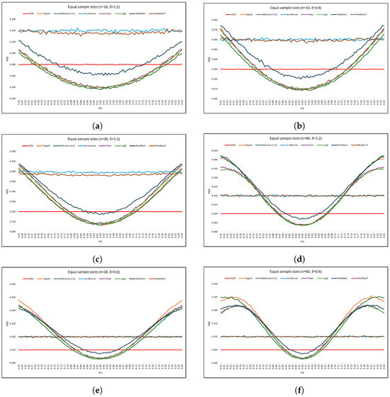
To evaluate the performance of the proposed preliminary test estimator (${\widehat{\mu }}_{PT}$) in comparison to the conventional single-stage estimator (${\widehat{\mu }}_{GD}$) using equal sample sizes ($n_1=n_2=n$) and a fixed significance level ($\alpha =0.05$), it is observed that as the sample size (n) increases, the MSE generally decreases. Notably, when μ is closer to the hypothesized mean (${\mu }_0$), the preliminary test estimator outperforms the unbiased estimator across various values of δ. This range of values where the preliminary test estimator excels can be referred to as its effective interval. After reaching a minimum at $\mu =0$, a slight rise in MSE is observed as μ deviates further from ${\mu }_0$. This trend is evident in the results depicted in Figure 1a,b, indicating that for $\delta =1.2$ and $\delta =0.6$, the proposed estimator performs better than the unbiased estimator when $-0.2\le \mu \le 0.2$. Conversely, for $\delta =1.2$ and $\delta =0.6$, the proposed estimator outperforms the unbiased estimator when $-0.12\le \mu \le 0.12$ and $-0.08\le \mu \le 0.08$, respectively (as shown in Figure 1c,e for $n=30$). Again, for $\delta =1.2$ and $\delta =0.6$, the proposed estimator outperforms the unbiased estimator when $-0.12\le \mu \le 0.12$ and $-0.06\le \mu \le 0.06$, respectively (as shown in Figure 1d,f for $n=60$). The preliminary test estimator, employing Tippett, Wilkinson (r = 2), Fisher’s inverse ${\chi }^2$, logit, and modified t tests, demonstrates satisfactory performance within its effective interval, as indicated by MSE values. These findings are consistent with the conclusions drawn by Kifle et al. (2021) regarding the efficacy of Fisher’s inverse ${\chi }^2$ and modified t tests across various sample sizes and significance levels [33].

5. Application in Biological Research

To demonstrate the practical applicability of the proposed preliminary test estimator, we analyzed data from four experiments used to estimate the percentage of albumin in plasma protein of normal human subjects. This dataset is reported in Meier [9] and appears in

Table 4. Albumin in plasma protein.

Experiment	${\mathit{n}}_{\mathit{i}}$	Mean	Variance
A	12	62.30	12.99
B	15	60.30	7.84
C	7	59.50	33.43
D	16	61.50	18.51

. For this dataset, previous studies focusing on the test problem [44,45], have compared the various test procedures for testing $H_1:\mu =59.50$ versus $H_2:\mu \ne 59.50$.

In our scenario, we could consider 59.50 as our non-sample prior information and apply our proposed preliminary test estimator to address this issue. According to the findings presented in

Table 5. The proposed test estimator for albumin in plasma protein with ${\mu }_0=59.50$.

${\widehat{\mathit{\mu }}}_{\mathit{GD}}$	${\widehat{\mathit{\mu }}}_{\mathit{PT}}^{\mathit{T}}$	${\widehat{\mathit{\mu }}}_{\mathit{PT}}^{\mathit{W}(\mathit{r}=2)}$	${\widehat{\mathit{\mu }}}_{\mathit{PT}}^{\mathit{W}(\mathit{r}=3)}$	${\widehat{\mathit{\mu }}}_{\mathit{PT}}^{\mathit{W}(\mathit{r}=4)}$	${\widehat{\mathit{\mu }}}_{\mathit{PT}}^{\mathit{IN}}$	${\widehat{\mathit{\mu }}}_{\mathit{PT}}^{\mathit{F}}$	${\widehat{\mathit{\mu }}}_{\mathit{PT}}^{\mathit{L}}$	${\widehat{\mathit{\mu }}}_{\mathit{PT}}^{\mathit{Mt}}$	${\widehat{\mathit{\mu }}}_{\mathit{PT}}^{\mathit{MF}}$
60.99	59.5	60.99	59.50	59.50	59.50	59.50	60.99	60.99	60.99

T: Tippett’s test, W: Wilkinson’s test, $IN$: Inverse normal test, F: Fisher’s inverse ${\chi }^2$-test. L: The logit test, $Mt$: Modified t test, $MF$: Modified F test.

, the estimated mean (${\widehat{\mu }}_{PT}$) derived from p-value based tests (including Tippett’s, Wilkinson ($r=3$ and $r=4$), Inverse normal, and Fisher’s tests) notably integrates the non-sample prior information.

In our second application of the proposed preliminary test estimator, we analyzed the data from four experiments about non-fat milk powder. This data set is reported by Eberhardt et al. [10] and appears in

Table 6. Selenium in non-fat milk powder.

Methods	${\mathit{n}}_{\mathit{i}}$	Mean	Variance
Atomic absorption spectrometry	8	105.00	85.71
Neutron activation:
(1.) Instrumental	12	109.75	20.75
(2.) Radiochemical	14	109.50	2.73
Isotope dilution mass spectrometry	8	113.25	33.64

. We can compute values of ${\mu }_{PT}$ for different values of ${\mu }_0$ with fixed sampling values, based on P-value and modified exact tests. The resulting values are shown in

Table 7. The proposed test estimator for selenium in non-fat milk powder for various values of ${\mu }_0$.

${\mathit{\mu }}_0$	${\widehat{\mathit{\mu }}}_{\mathit{GD}}$	${\widehat{\mathit{\mu }}}_{\mathit{PT}}^{\mathit{T}}$	${\widehat{\mathit{\mu }}}_{\mathit{PT}}^{\mathit{W}(\mathit{r}=2)}$	${\widehat{\mathit{\mu }}}_{\mathit{PT}}^{\mathit{W}(\mathit{r}=3)}$	${\widehat{\mathit{\mu }}}_{\mathit{PT}}^{\mathit{W}(\mathit{r}=4)}$	${\widehat{\mathit{\mu }}}_{\mathit{PT}}^{\mathit{IN}}$	${\widehat{\mathit{\mu }}}_{\mathit{PT}}^{\mathit{F}}$	${\widehat{\mathit{\mu }}}_{\mathit{PT}}^{\mathit{L}}$	${\widehat{\mathit{\mu }}}_{\mathit{PT}}^{\mathit{Mt}}$	${\widehat{\mathit{\mu }}}_{\mathit{PT}}^{\mathit{MF}}$
90.00	109.60	109.60	109.60	109.60	109.60	109.60	109.60	109.60	109.60	109.60
100.00	109.60	109.60	109.60	109.60	109.60	109.60	109.60	109.60	109.60	109.60
110.00	109.60	110.00	110.00	110.00	110.00	109.60	110.00	110.00	109.60	109.60
110.50	109.60	110.50	110.50	110.50	110.50	109.60	110.50	110.50	109.60	109.60
111.00	109.60	109.60	111.00	111.00	109.60	109.60	109.60	109.60	109.60	111.00

T: Tippett’s test, W: Wilkinson’s test, $IN$: Inverse normal test, F: Fisher’s inverse ${\chi }^2$-test. L: The logit test, $Mt$: Modified t test, $MF$: Modified F test.

.

The findings presented in Table 7 suggest that when ${\mu }_0$ is below 110.00, ${\widehat{\mu }}_{PT}={\widehat{\mu }}_{GD}$. However, when ${\mu }_0$ falls within the range of 110.00 to 110.50, tests including Tippett’s, Wilkinson’s ($r=2$, $r=3$, and $r=4$), Fisher’s, and the logit tests do not reject the null hypothesis ($H_0$), indicating an estimated common mean $\left(\mu \right)$ of equal to 110.00, whereas other tests reject $H_0$, estimating the common mean $\mu$ equal to 109.60. For ${\mu }_0=111.00$, tests based on Wilkinson’s ($r=2$ and $r=3$) and the modified F tests also fail to reject $H_0$, with an estimated $\mu$ equal to 110.00. Both the Inverse normal test and the Modified t test accepted the null hypothesis for various values of ${\mu }_0$. This may be because the Inverse normal test transforms p-values into z-scores and combines them, whereas the Modified t test adjusts the traditional t test procedure to address specific issues such as heteroscedasticity or small sample sizes.

From the above results, we do not intend to make any broad conclusions here, but our simulation results suggest that our proposed preliminary test estimator based on Tippett’s, Wilkinson’s ($r=2$, $r=3$, and $r=4$), Fisher’s, and the logit tests are feasible and could be applied to this specific case if prior information about the population mean is available.

6. Conclusions

The past decade has witnessed increased interest in estimating unknown quantities using data from multiple independent yet non-homogeneous samples. This approach finds application across various domains, as evidenced by the diverse range of applications discussed in the most recent book by Sinah et al. [2]. In this study, we introduce a preliminary test estimator that integrates non-sample prior information. Our simulations indicate that this proposed estimator exhibits distinct advantages in certain scenarios, particularly when dealing with very small sample sizes and situations where ${\sigma }_2^2$ exceeds ${\sigma }_1^2$. Notably, the proposed estimator significantly reduces MSE values compared to traditional unbiased estimators, especially when $\mu$ is in proximity to ${\mu }_0$. Moreover, the performance of the proposed estimator, when based on Tippett’s, Wilkinson’s ($r=2$, $r=3$, and $r=4$), Fisher’s, and logit tests, surpasses that of ${\widehat{\mu }}_{GD}$, particularly in cases involving very small sample sizes. For substantial sample sizes, the effectiveness of the suggested estimator, deploying Inverse normal and modified F tests, appeared to demonstrate consistent and dependable performance, MSE discrepancy of less than $0.02$ compared to the MSE of the unbiased estimator. Consequently, we advocate for the adoption of the proposed estimator to enhance the accuracy of $\mu$ estimation. Nevertheless, no universally optimal estimator performs best across all scenarios. Consequently, it becomes crucial to select an appropriate estimator tailored to each specific scenario. The decision on which estimator to employ relies on the objectives of the research, making it challenging to devise a purely statistical strategy for selection. Our findings in this article suggest that through careful application to real meta-analyses, the proposed estimator exhibits promising potential.

This article primarily considered the scenario under the general preliminary test estimator whereby ${\alpha }_1={\alpha }_2=\alpha$. Extensions of this work could explore cases where ${\alpha }_1=0$ and ${\alpha }_2=1$ through the introduction of a randomized test, where the probability function $q(·)$ is treated as a shrinkage parameter. Consequently, the proposed estimator would transition to a non-randomized form [25]. Additionally, it’s pertinent to highlight that this study focuses on the univariate common mean of multiple normal populations. Future extensions could broaden the scope to encompass multiple responses, such as bivariate common mean.

References

- Wang, X.M.; Zhang, X.R.; Li, Z.H.; Zhong, W.F.; Yang, P.; Mao, C. A brief introduction of meta-analyses in clinical practice and research. J. Gene Med. 2021, 23, e3312. [Google Scholar] [CrossRef] [PubMed]
- Sinha, B.K.; Hartung, J.; Knapp, G. Statistical Meta-Analysis with Applications; John Wiley & Sons: Hoboken, NJ, USA, 2011. [Google Scholar]
- Haidich, A.B. Meta-analysis in medical research. Hippokratia 2010, 14, 29. [Google Scholar] [PubMed]
- Glass, G.V. Primary, secondary, and meta-analysis of research. Educ. Res. 1976, 5, 3–8. [Google Scholar] [CrossRef]
- DerSimonian, R.; Laird, N. Evaluating the effect of coaching on SAT scores: A meta-analysis. Harv. Educ. Rev. 1983, 53, 1–15. [Google Scholar] [CrossRef]
- Hedges, L.V. Advances in statistical methods for meta-analysis. New Dir. Program Eval. 1984, 24, 25–42. [Google Scholar] [CrossRef]
- Liu, Q.; Qin, C.; Liu, M.; Liu, J. Effectiveness and safety of SARS-CoV-2 vaccine in real-world studies: A systematic review and meta-analysis. Infect. Dis. Poverty 2021, 10, 132. [Google Scholar] [CrossRef]
- Watanabe, A.; Kani, R.; Iwagami, M.; Takagi, H.; Yasuhara, J.; Kuno, T. Assessment of efficacy and safety of mRNA COVID-19 vaccines in children aged 5 to 11 years: A systematic review and meta-analysis. JAMA Pediatr. 2023, 177, 384–394. [Google Scholar] [CrossRef]
- Meier, P. Variance of a weighted mean. Biometrics 1953, 9, 59–73. [Google Scholar] [CrossRef]
- Eberhardt, K.R.; Reeve, C.P.; Spiegelman, C.H. A minimax approach to combining means, with practical examples. Chemom. Intell. Lab. Syst. 1989, 5, 129–148. [Google Scholar] [CrossRef]
- Graybill, F.A.; Deal, R. Combining unbiased estimators. Biometrics 1959, 15, 543–550. [Google Scholar] [CrossRef]
- Kubokawa, T. Admissible minimax estimation of a common mean of two normal populations. Ann. Stat. 1987, 1245–1256. [Google Scholar] [CrossRef]
- Brown, L.D.; Cohen, A. Point and confidence estimation of a common mean and recovery of interblock information. Ann. Stat. 1974, 2, 963–976. [Google Scholar] [CrossRef]
- Cohen, A.; Sackrowitz, H.B. On estimating the common mean of two normal distributions. Ann. Stat. 1974, 1274–1282. [Google Scholar] [CrossRef]
- Moore, B.; Krishnamoorthy, K. Combining independent normal sample means by weighting with their standard errors. J. Stat. Comput. Simul. 1997, 58, 145–153. [Google Scholar] [CrossRef]
- Huang, H. Combining estimators in interlaboratory studies and meta-analyses. Res. Synth. Methods 2023, 14, 526–543. [Google Scholar] [CrossRef] [PubMed]
- Dong, Y.F.; Chen, W.X.; Xie, M.Y. Best linear unbiased estimators of location and scale ranked set parameters under moving extremes sampling design. Acta Math. Appl. Sin. Engl. Ser. 2023, 39, 222–231. [Google Scholar] [CrossRef]
- Khatun, H.; Tripathy, M.R.; Pal, N. Hypothesis testing and interval estimation for quantiles of two normal populations with a common mean. Commun. Stat.-Theory Methods 2022, 51, 5692–5713. [Google Scholar] [CrossRef]
- Marić, N.; Graybill, F.A. Evaluation of a method for setting confidence intervals on the common mean of two normal populations. Commun. Stat.-Simul. Comput. 1979, 8, 53–60. [Google Scholar] [CrossRef]
- Pagurova, V.I.; Gurskii, V. A confidence interval for the common mean of several normal distributions. Theory Probab. Appl. 1980, 24, 882–888. [Google Scholar] [CrossRef]
- Krishnamoorthy, K.; Moore, B.C. Combining information for prediction in linear regression. Metrika 2002, 56, 73–81. [Google Scholar] [CrossRef]
- Bancroft, T.A. On biases in estimation due to the use of preliminary tests of significance. Ann. Math. Stat. 1944, 15, 190–204. [Google Scholar] [CrossRef]
- Stein, C. Inadmissibility of the usual estimator for the mean of a multivariate normal distribution. In Proceedings of the Third Berkeley Symposium on Mathematical Statistics and Probability, Volume 1: Contributions to the Theory of Statistic, 26–31 December 1954; University of California Press: Berkeley, CA, USA, 1956; Volume 3, pp. 197–207. [Google Scholar]
- Khan, S.; Saleh, A.M.E. On the comparison of the pre-test and shrinkage estimators for the univariate normal mean. Stat. Pap. 2001, 42, 451–473. [Google Scholar] [CrossRef]
- Shih, J.H.; Konno, Y.; Chang, Y.T.; Emura, T. A class of general pretest estimators for the univariate normal mean. Commun. Stat.-Theory Methods 2023, 52, 2538–2561. [Google Scholar] [CrossRef]
- Taketomi, N.; Konno, Y.; Chang, Y.T.; Emura, T. A meta-analysis for simultaneously estimating individual means with shrinkage, isotonic regression and pretests. Axioms 2021, 10, 267. [Google Scholar] [CrossRef]
- Thompson, J.R. Some shrinkage techniques for estimating the mean. J. Am. Stat. Assoc. 1968, 63, 113–122. [Google Scholar] [CrossRef]
- Mphekgwana, P.M.; Kifle, Y.G.; Marange, C.S. Shrinkage Testimator for the Common Mean of Several Univariate Normal Populations. Mathematics 2024, 12, 1095. [Google Scholar] [CrossRef]
- Pal, N.; Lin, J.J.; Chang, C.H.; Kumar, S. A revisit to the common mean problem: Comparing the maximum likelihood estimator with the Graybill–Deal estimator. Comput. Stat. Data Anal. 2007, 51, 5673–5681. [Google Scholar] [CrossRef]
- Khatri, C.; Shah, K. Estimation of location parameters from two linear models under normality. Commun. Stat.-Theory Methods 1974, 3, 647–663. [Google Scholar]
- Sinha, B.K. Unbiased estimation of the variance of the Graybill-Deal estimator of the common mean of several normal populations. Can. J. Stat. 1985, 13, 243–247. [Google Scholar] [CrossRef]
- Hartung, J. An alternative method for meta-analysis. Biom. J. J. Math. Methods Biosci. 1999, 41, 901–916. [Google Scholar] [CrossRef]
- Kifle, Y.G.; Moluh, A.M.; Sinha, B.K. Comparison of local powers of some exact tests for a common normal mean with unequal variances. In Methodology and Applications of Statistics; Springer: Berlin/Heidelberg, Germany, 2021; pp. 77–101. [Google Scholar]
- Kifle, Y.G.; Moluh, A.M.; Sinha, B.K. Inference about a Common Mean Vector from Several Independent Multinormal Populations with Unequal and Unknown Dispersion Matrices. Mathematics 2024, 12, 2723. [Google Scholar] [CrossRef]
- Cohen, A.; Sackrowitz, H. Exact tests that recover interblock information in balanced incomplete blocks designs. J. Am. Stat. Assoc. 1989, 84, 556–559. [Google Scholar] [CrossRef]
- Tippett, L.H.C. The Methods of Statistics: An Introduction Mainly for Workers in the Biological Sciences; Williams & Norgate: London, UK, 1931. [Google Scholar]
- Wilkinson, B. A statistical consideration in psychological research. Psychol. Bull. 1951, 48, 156. [Google Scholar] [CrossRef] [PubMed]
- Stouffer, S.A.; Suchman, E.A.; DeVinney, L.C.; Star, S.A.; Williams, R.M., Jr. The American Soldier: Adjustment during Army Life. (Studies in Social Psychology in World War ii); Princeton University Press: Princeton, NJ, USA, 1949; Volume 1. [Google Scholar]
- Fisher, R. Statistical Methods for Research Workers, 4th ed.; Oliver and Boyd: Edinburgh, Scotland; London, UK, 1932. [Google Scholar]
- George, E.O.; Mudholkar, G.S. The Logit Method for Combining Tests; Technical Report; Department of Statistics, Rochester University: Rochester, NY, USA, 1979. [Google Scholar]
- Fairweather, W.R. A method of obtaining an exact confidence interval for the common mean of several normal populations. J. R. Stat. Soc. Ser. (Appl. Stat.) 1972, 21, 229–233. [Google Scholar] [CrossRef]
- Jordan, S.M.; Krishnamoorthy, K. Exact confidence intervals for the common mean of several normal populations. Biometrics 1996, 52, 77–86. [Google Scholar] [CrossRef]
- R Core Team. R: A Language and Environment for Statistical Computing; R Foundation for Statistical Computing: Vienna, Austria, 2021. [Google Scholar]
- Chang, C.H.; Pal, N. Testing on the common mean of several normal distributions. Comput. Stat. Data Anal. 2008, 53, 321–333. [Google Scholar] [CrossRef]
- Li, X.; Williamson, P.P. Testing on the common mean of normal distributions using Bayesian methods. J. Stat. Comput. Simul. 2014, 84, 1363–1380. [Google Scholar] [CrossRef]
Disclaimer/Publisher’s Note: The statements, opinions and data contained in all publications are solely those of the individual author(s) and contributor(s) and not of MDPI and/or the editor(s). MDPI and/or the editor(s) disclaim responsibility for any injury to people or property resulting from any ideas, methods, instructions or products referred to in the content. |
© 2024 by the authors. Licensee MDPI, Basel, Switzerland. This article is an open access article distributed under the terms and conditions of the Creative Commons Attribution (CC BY) license (https://creativecommons.org/licenses/by/4.0/).