A New Methodology for the Development of Efficient Multistep Methods for First–Order IVPs with Oscillating Solutions IV: The Case of the Backward Differentiation Formulae

Abstract

A theory for the calculation of the phase–lag and amplification–factor for explicit and implicit multistep techniques for first–order differential equations was recently established by the author. His presentation also covered how the approaches’ efficacy is affected by the elimination of the phase–lag and amplification–factor derivatives. This paper will apply the theory for computing the phase–lag and amplification–factor, originally developed for implicit multistep methods, to a subset of implicit methods, called backward differentiation formulae (BDF), and will examine the impact of the phase–lag and amplification–factor derivatives on the efficiency of these strategies. Next, we will show you the stability zones of these brand-new approaches. Lastly, we will discuss the results of numerical experiments and draw some conclusions about the established approaches.

1. Introduction

An equation or system of equations that looks like this:

$${\mathsf{\Psi }}^{\prime }\left(\mathbf{t}\right)=\mathbf{Q}(\mathbf{t},\mathsf{\Psi }),\mathsf{\Psi }\left({\mathbf{t}}_{\mathbf{0}}\right)={\mathsf{\Psi }}_{\mathbf{0}}.$$

(1)

Astrophysics, electronics, materials science, chemistry, physics, and nanotechnology are just a few of the fields that make use of these compounds. See references [1,2] for further information on the class of equations with oscillatory or periodic solutions.

Over the last two decades, several efforts have been made to determine the numerical solution to the specified problem or set of equations (for instances, refer to [3,4,5,6,7], and the cited works therein). Refer to [3,4], and the cited works for a more in-depth analysis of the techniques used to solve (1) with solutions that display oscillating behavior; for example, Quinlan and Tremaine [5]. Certain characteristics define the numerical strategies found in the literature for solving (1), the most prominent of which is that they are either multistep or hybrid approaches. Additionally, the majority of these techniques were developed for numerically solving second-order differential equations. Along with their corresponding bibliographies, the following theoretical frameworks for research are discussed:

• Runge–Kutta and Runge–Kutta-Nyström methods with minimal phase–lag, as well as exponentially–fitted, trigonometrically–fitted, phase–fitted, and amplification–fitted variations of these methods (see [8,9,10,11,12,13,14,15])
• Amplification–Fitted Multistep Methods, Multistep Methods with Minimal Phase–Lag, Phase–Fitted Methods and Methods that are Trigonometrically or Exponentially Fitted (see [16,17,18,19,20,21,22,23,24,25,26])

Recently, Simos developed the theory for building first–order IVPs using multistep procedures with minimal phase–lag or phase–fitted methods in his publications [27,28,29]. More specifically, he developed his theory for estimating the phase–lag and amplification error of multistep techniques for first–order IVPs (explicit [27], implicit [28]) and the effect of removing the derivatives of the phase–lag and amplification–factor on the efficacy of the method [29]. On the topic of backward differentiation formulae ($BDF$) for second–order IVPs with oscillating solutions, Saadat et al. [30] has also recently put forward a theory. In particular, $BDF$ techniques are known to be implicit and built for stiff issues. It is possible to use the phase–fitted and amplification–fitted techniques to very long integration intervals. None of the instances in the study [30] had integration areas larger than $\left[0,10\pi \right]$. The behavior of the specified approaches in intervals $\left[0,50000\pi \right]$ or $\left[0,100000\pi \right]$ would be interesting to see.

In this study, we will utilize the theory that has been established for implicit multistep methods for first-order IVPs [28] to analyze BDF approaches and create efficient algorithms for this specific type of implicit multistep method. Additionally, we will examine the impact of phase–lag and amplification–factor derivatives on the efficacy of BDF methods for first-order IVPs.

Here is how the paper is structured:

• The theory for determining the phase–lag and amplification–factor of backward differentiation formulae (BDF) was established in Section 2. The theory presented in [28] will serve as the foundation for the development of the general theory since these techniques belong to a specific class of implicit multistep methods. We shall generate the direct equations for the phase–lag and amplification–factor calculations here.
• Section 3 presents the methodologies which will be used for the development of the new backward differentiation formulae (BDF).
• Section 4 introduces the Backward Differentiation Formula that will be used to examine.
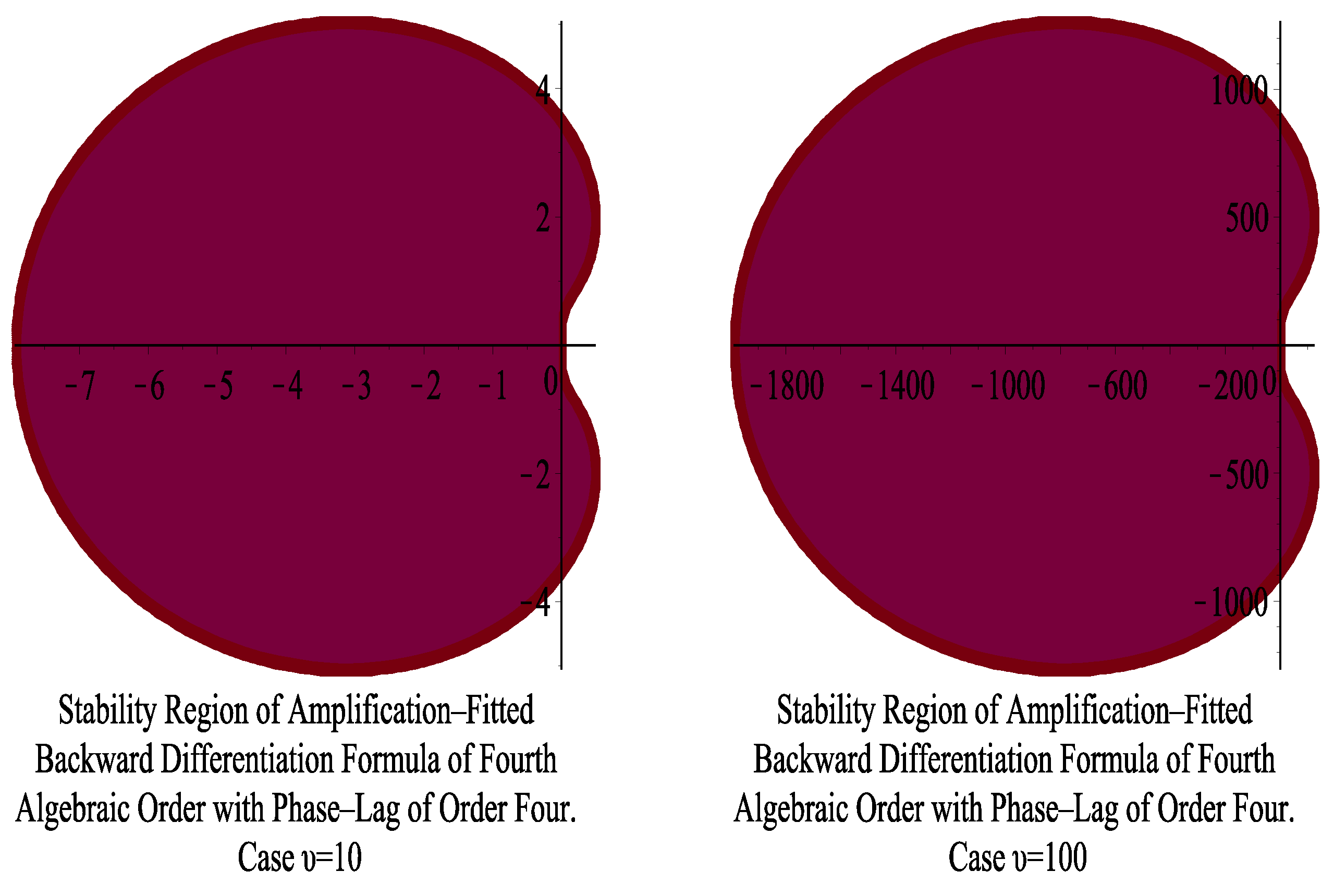
• Section 5 studies the amplification–fitted backward differentiation formula of fourth algebraic order with phase–lag of order four.
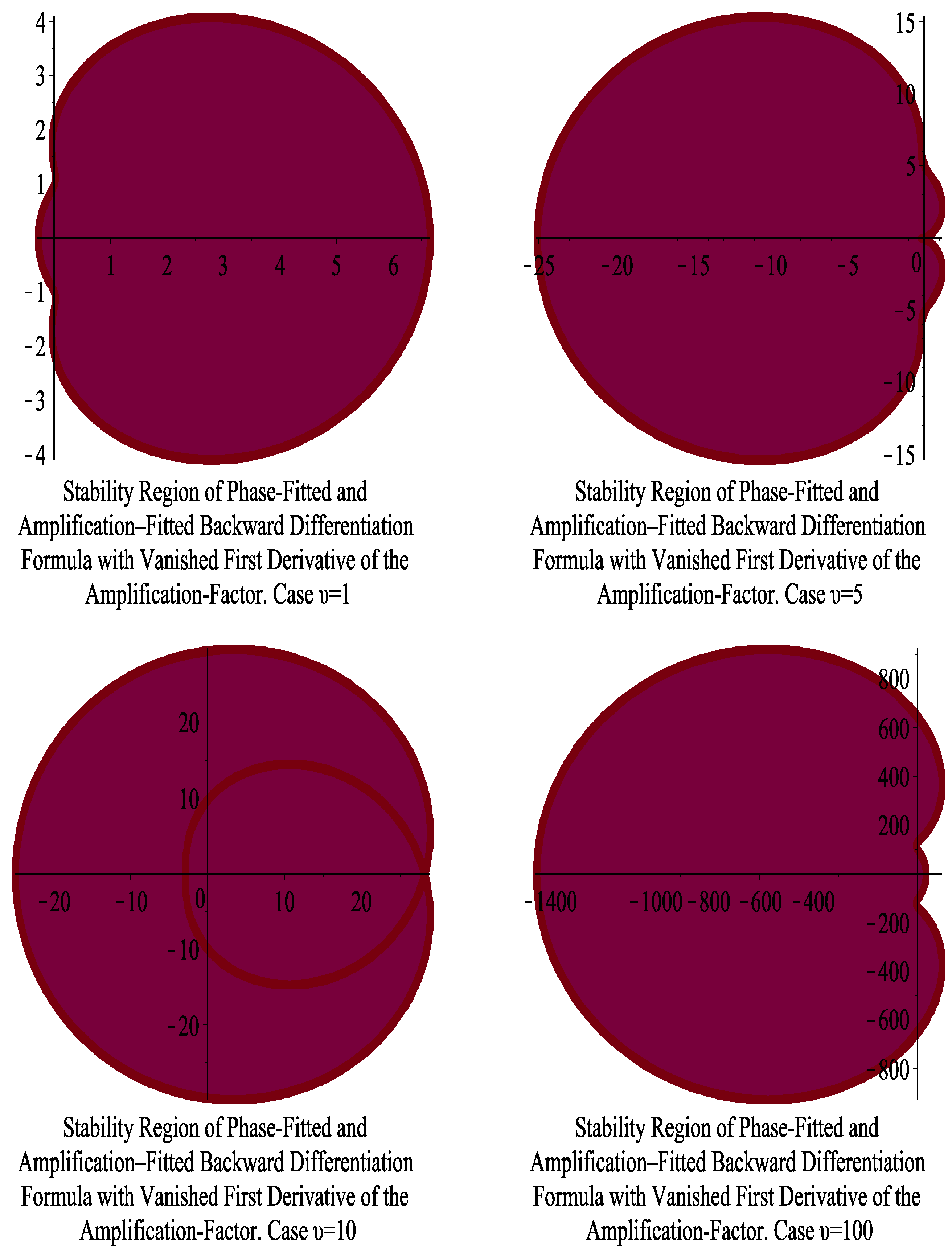
• Section 6 studies the phase–fitted and amplification–fitted backward differentiation formula of fourth algebraic order with elimination of the first derivative of the amplification–factor.
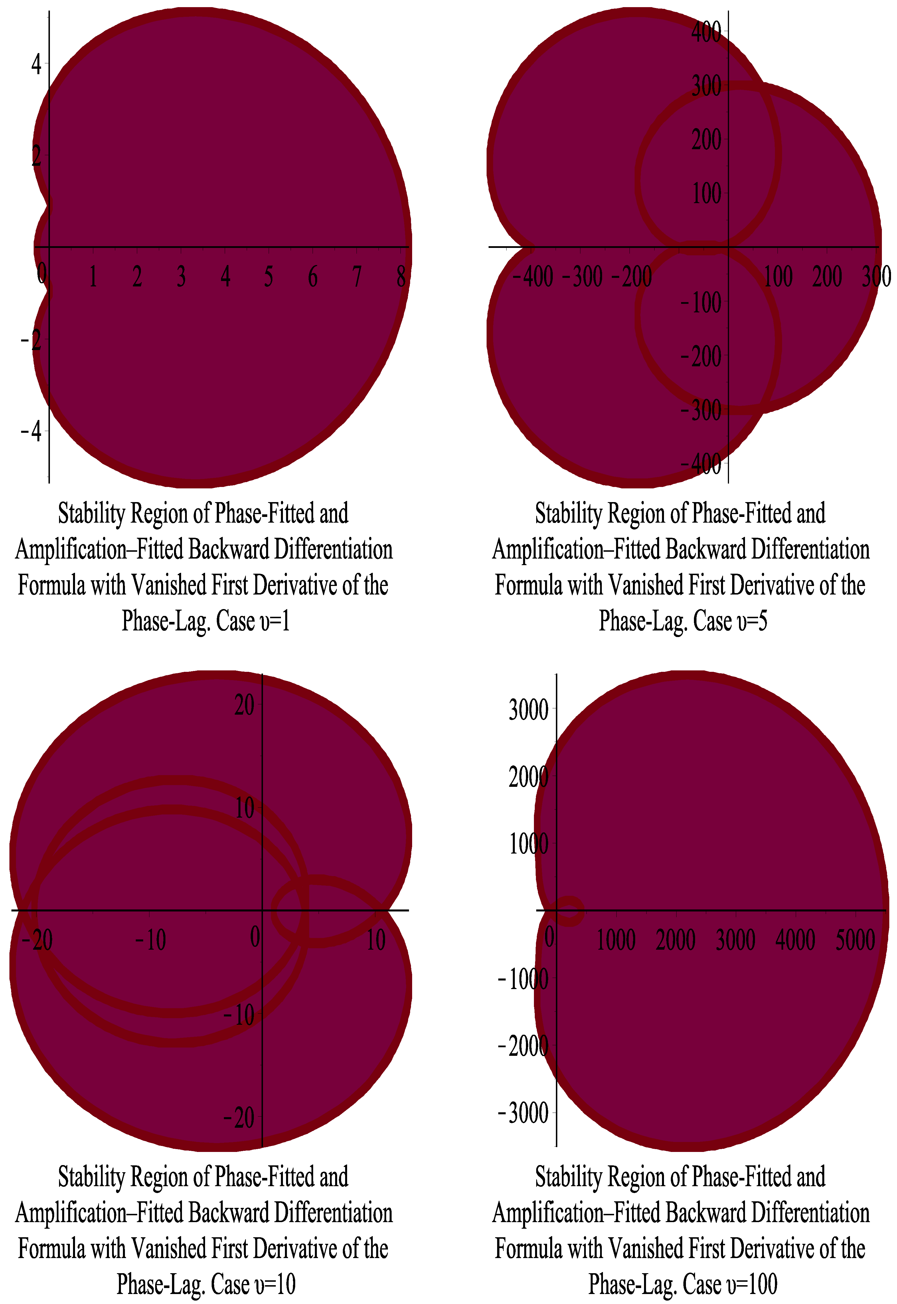
• Section 7 studies the phase–fitted and amplification–fitted backward differentiation formula of fourth algebraic order with the elimination of the first derivative of the phase–lag.
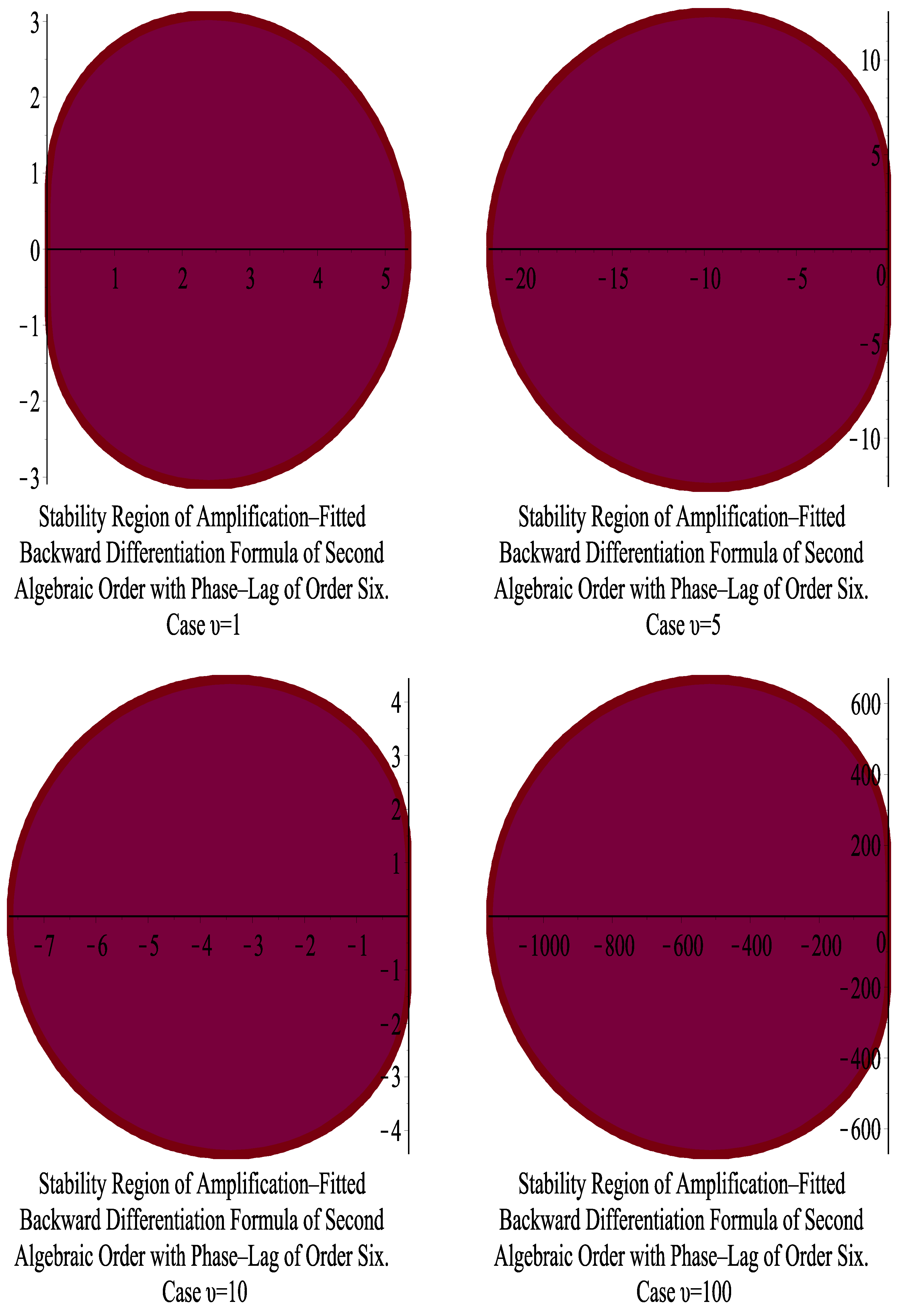
• Section 8 studies the amplification–fitted backward differentiation formula of second algebraic order with phase–lag of order six.
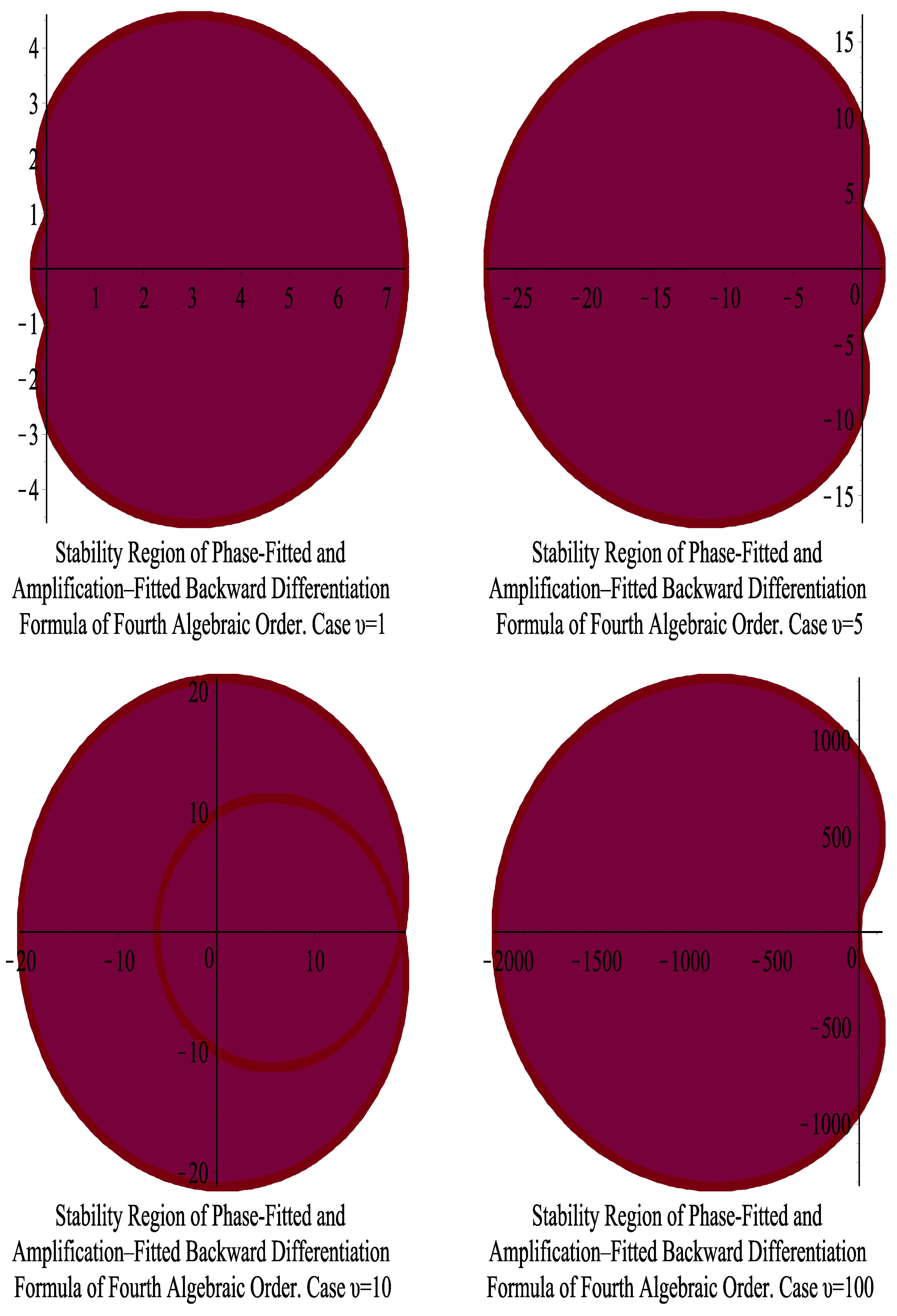
• Section 9 studies the phase–fitted and amplification–fitted backward differentiation formula of fourth algebraic order.
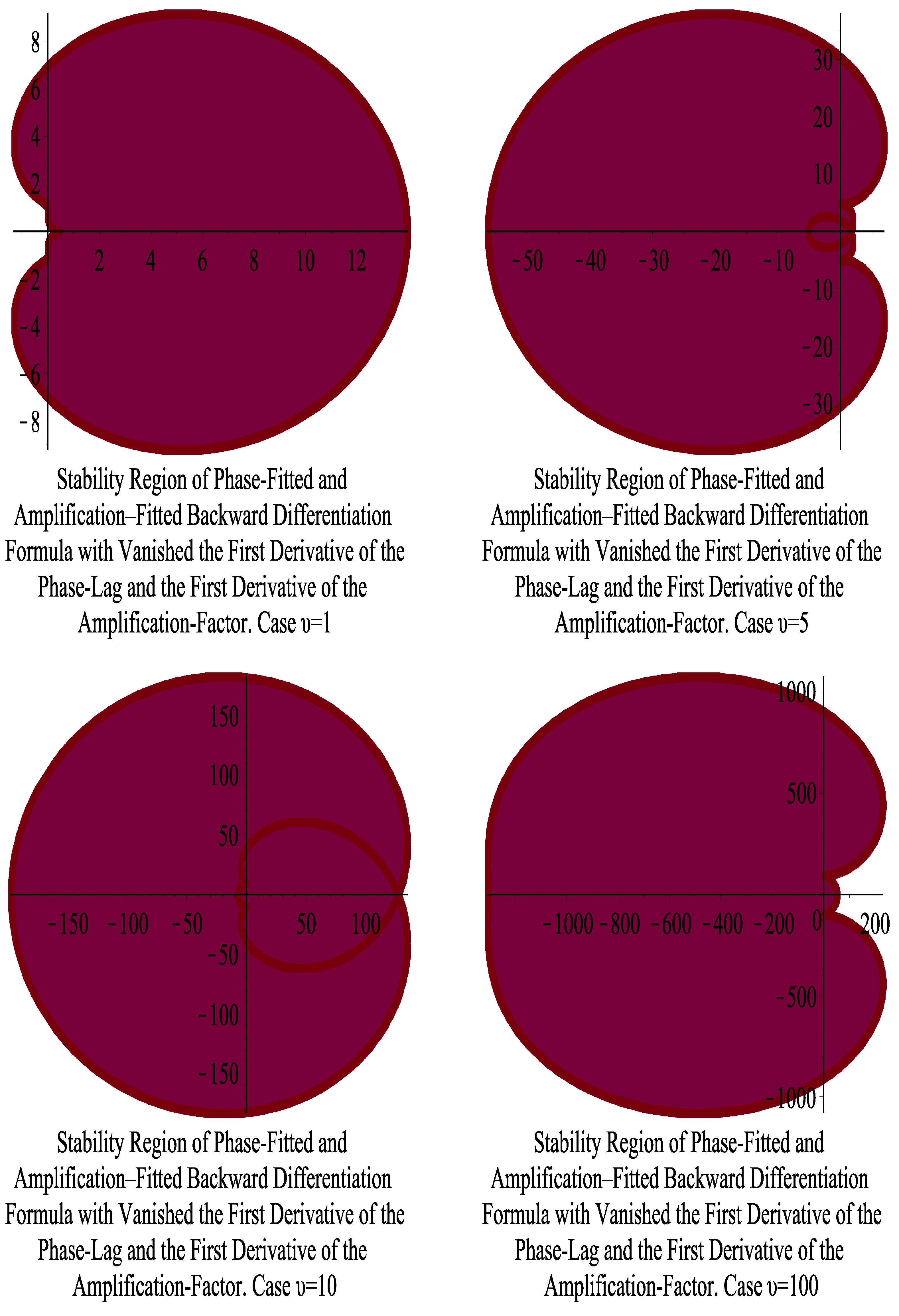
• Section 10 studies the phase–fitted and amplification–fitted backward differentiation formula of fourth algebraic order with the elimination of the first derivative of the phase–lag and the first derivative of the amplification–factor.
• In Section 11, we examine the stability of the newly acquired algorithms.
• In Section 12, we present several numerical examples and we comment on the numerical results.
• We provide the numerical results and conclusions in Section 13.

2. The Theory

2.1. Direct Formulae for Computation of the Phase–Lag and Amplification–Factor of Backward Differentiation Formulae

The theory for the development of direct formulae for the calculation of the phase–lag and amplification–factor of Backward Differentiation Formulae is based on the theory developed in the papers [27,28].

We consider the general form of the Backward Differentiation Formulae (BDF):

$$\sum _{j=0}^m{a}_j{\mathsf{\Psi }}_{n+j}=h{A}_m{\mathsf{\Psi }}_{n+m}^{\prime }.$$

(2)

We may analyze the phase–lag of the implicit multistep techniques (2) for the issues (1) using the scalar test equation that follows.

$${\mathsf{\Psi }}^{\prime }\left(t\right)=I\omega \mathsf{\Psi }\left(t\right).$$

(3)

where h is the step size of the integration, and $I=\sqrt{-1}$

The following formula may be used to solve this problem:

$$\mathsf{\Psi }\left(t\right)=exp\left(I\omega t\right).$$

(4)

Applying Formula (2) to Equation (3) we obtain:

$$\sum _{j=0}^m{a}_j{\mathsf{\Psi }}_{n+j}=hI\omega A_m\left(\omega h\right){\mathsf{\Psi }}_{n+m}.$$

(5)

Considering:

$$\upsilon =\omega h,$$

(6)

Equation (5) gives:

$$\left(a_m-I\upsilon A_m\left(\upsilon \right)\right){\mathsf{\Psi }}_{n+m}+\sum _{j=0}^{m-1}{a}_j{\mathsf{\Psi }}_{n+j}=0.$$

(7)

The difference equation described in (7) has the following characteristic equation:

$$\left[a_m-I\upsilon A_{n+m}\left(\upsilon \right)\right]{\lambda }^m+\sum _{j=0}^{m-1}{a}_j{\lambda }_j=0.$$

(8)

Definition 1. 

Given that the theoretical solution of the scalar test Equation (3) for $t=h$ is $exp\left(I\omega h\right)$, which can also be expressed as $exp\left(I\upsilon \right)$ (see (6)), and the numerical solution of the scalar test Equation (3) for $t=h$ is $exp\left(I\theta \left(\upsilon \right)\right)$, we can define the phase–lag in the following way:

$$\mathsf{\Phi }=\upsilon -\theta \left(\upsilon \right).$$

(9)

Given that $\upsilon ⟶0$, the phase–lag order is q if and only if $\mathsf{\Phi }=O\left({\upsilon }^{q+1}\right)$, and $\theta \left(\upsilon \right)$ is an approximated value of υ produced by the numerical solution.

Taking into account what is below:

$${\lambda }^n={exp}^{nI\theta \left(\upsilon \right)}=cos\left[n\theta \left(\upsilon \right)\right]+Isin\left[n\theta \left(\upsilon \right)\right]n=1,2,\dots ,$$

(10)

we obtain:

$$\begin{array}{c}\hfill \left[a_m-I\upsilon A_m\left(\upsilon \right)\right]\left\{cos\left[m\theta \left(\upsilon \right)\right]+Isin\left[m\theta \left(\upsilon \right)\right]\right\}\\ \hfill +\sum _{j=0}^{m-1}{a}_j\left\{cos\left[j\theta \left(\upsilon \right)\right]+Isin\left[j\theta \left(\upsilon \right)\right]\right\}=0.\end{array}$$

(11)

It is necessary to apply the following lemmas to comprehend the connection provided in the Formula (11).

Lemma 1. 

These relations are true:

$$cos\left[\theta \left(\upsilon \right)\right]=cos\left(\upsilon \right)+c{\upsilon }^{q+2}+O\left({\upsilon }^{q+4}\right).$$

(12)

$$sin\left[\theta \left(\upsilon \right)\right]=sin\left(\upsilon \right)-c{\upsilon }^{q+1}+O\left({\upsilon }^{q+3}\right).$$

(13)

For the proof, see [27].

Lemma 2. 

This relation holds:

$$\begin{array}{c}\hfill cos\left[j\theta \left(\upsilon \right)\right]=cos\left(j\upsilon \right)+c{j}^2{\upsilon }^{q+2}+O\left({\upsilon }^{q+4}\right).\end{array}$$

(14)

$$\begin{array}{c}\hfill sin\left[j\theta \left(\upsilon \right)\right]=sin\left(j\upsilon \right)-cj{\upsilon }^{q+1}+O\left({\upsilon }^{q+3}\right).\end{array}$$

(15)

For the proof, see [27].

When the relations (14) and (15) are considered, the relation (11) shifts to:

$$\begin{array}{c}\hfill \left\{cos\left(m\upsilon \right)+c{m}^2{\upsilon }^{q+2}+I\left[sin\left(m\upsilon \right)-cm{\upsilon }^{q+1}\right]\right\}\left(a_m-I\upsilon A_m\left(\upsilon \right)\right)\\ \hfill +\sum _{j=0}^{m-1}{a}_j\left\{cos\left(j\upsilon \right)+c{j}^2{\upsilon }^{q+2}+I\left[sin\left(j\upsilon \right)-cj{\upsilon }^{q+1}\right]\right\}=0.\end{array}$$

(16)

Dividing the previously given connection (16) into two halves, real and imaginary, is obviously conceivable.

2.1.1. The Real Part

The real part gives:

$$\begin{array}{c}\hfill a_{m}cos\left(m\upsilon \right)+a_{m}c{m}^2{v}^{q+2}+\upsilon A_m\left(\upsilon \right)sin\left(m\upsilon \right)\\ \hfill -\upsilon A_m\left(\upsilon \right)cm{\upsilon }^{q+1}+\sum _{j=0}^{m-1}{a}_{j}cos\left(j\upsilon \right)+\sum _{j=0}^{m-1}{a}_{j}c{j}^2{\upsilon }^{q+2}=0.\end{array}$$

(17)

The relation (17) gives:

$$\begin{array}{c}\hfill a_{m}cos\left(m\upsilon \right)+\upsilon A_m\left(\upsilon \right)sin\left(m\upsilon \right)+\sum _{j=0}^{m-1}{a}_{j}cos\left(j\upsilon \right)\\ \hfill =-c{\upsilon }^{q+2}\left[a_m{m}^2-m{A}_m\left(\upsilon \right)+\sum _{j=0}^{m-1}{a}_j{j}^2\right]⟹\\ \hfill -c{\upsilon }^{q+2}={\displaystyle \frac{a_{m}cos\left(m\upsilon \right)+\upsilon A_m\left(\upsilon \right)sin\left(m\upsilon \right)+{\sum }_{j=0}^{m-1}{a}_{j}cos\left(j\upsilon \right)}{a_m{m}^2-m{A}_m\left(\upsilon \right)+{\sum }_{j=0}^{m-1}{a}_j{j}^2}}.\end{array}$$

(18)

Ref. (2) states that this is the direct formula for determining the phase–lag of the Backward Differentiation Formulae. We will describe how to determine the phase–lag of the method (2) in the next sections.

2.1.2. The Imaginary Part

The imaginary part gives:

$$\begin{array}{c}\hfill a_{m}sin\left(m\upsilon \right)-a_{m}cm{\upsilon }^{q+1}-\upsilon A_m\left(\upsilon \right)cos\left(m\upsilon \right)\\ \hfill -\upsilon A_m\left(\upsilon \right)c{m}^2{\upsilon }^{q+2}+\sum _{j=0}^{m-1}{a}_j\left[sin\left(j\upsilon \right)-cj{\upsilon }^{q+1}\right]=0.\end{array}$$

(19)

The relation (19) gives:

$$\begin{array}{c}\hfill a_{m}sin\left(m\upsilon \right)+\sum _{j=0}^{m-1}{a}_{j}sin\left(j\upsilon \right)-\upsilon A_m\left(\upsilon \right)cos\left(m\upsilon \right)\\ \hfill =-c{\upsilon }^{q+1}\left[-a_{m}m-\sum _{j=0}^{m-1}{a}_{j}j-A_m{m}^2{\upsilon }^2\right]⟹\\ \hfill -c{\upsilon }^{q+1}={\displaystyle \frac{a_{m}sin\left(m\upsilon \right)+{\sum }_{j=0}^{m-1}{a}_{j}sin\left(j\upsilon \right)-\upsilon A_m\left(\upsilon \right)cos\left(m\upsilon \right)}{-a_{m}m-{\sum }_{j=0}^{m-1}{a}_{j}j-A_m{m}^2{\upsilon }^2}}.\end{array}$$

(20)

Ref. (2) states that this is the direct formula for determining the amplification–factor of the Backward Differentiation Formulae. We will describe how to determine the amplification–factor of the method (2) in the next sections.

Definition 2. 

We refer to the algorithm that has eliminated phase–lag as the phase–fitted method.

Definition 3. 

The technique where the amplification–factor has disappeared is referred to as the amplification–fitted approach.

2.2. The Role of the Derivatives of the Phase–Lag and Derivatives of the Amplification–Factor on the Efficiency of BDF Algorithms

For the role of the derivatives of the phase–lag and amplification–factor on the efficiency of generally multistep methods (and consequently, of Backward Differentiation Formulae), one can see in [29].

We use the following approach to vanish of the phase–lag and amplification–factor derivatives:

• We determine the method’s phase–lag and amplification–factor using Formula (18) and (20), respectively.
• The formulae generated in the prior stage are differentiated on $\upsilon$.
• For the derivatives of the phase–lag and the amplification–factor that were generated in the preceding stages, we request that they be set equal to zero.

We provide straightforward equations in Appendix A for calculating the derivatives of the phase–lag and the amplification–factor. These formulae were developed by differentiating the Formulae (18) and (20) on $\upsilon$.

3. Minimizing or Eliminating the Phase–Lag and the Amplification–Factor and the Derivatives of the Phase–Lag and the Amplification–Factor

Methodologies for eliminating the phase–lag and the amplification–factor as well as methodologies for eliminating phase–lag and amplification–factor derivatives will be presented in this paper.

To be more precise, we will be presenting methodologies for:

• Minimization of the phase–lag
• Eliminating the phase–lag
• Eliminating the amplification–factor
• Eliminating the derivative of the phase–lag
• Eliminating the derivative of the amplification–factor
• Eliminating the derivatives of the phase–lag and the amplification–factor

We note here that all the above methodologies lead to an amplification–fitted method.

4. Backward Differentiation Formulae (BDF)

In this section, we present the Backward Differentiation Formula on which we will present the methodologies for eliminating the phase–lag, amplification–factor, derivative of the phase–lag, and derivative of the amplification–factor.

We will analyze the backward differentiation formula of the form:

$${\mathsf{\Psi }}_{n+2}+{\kappa }_3{\mathsf{\Psi }}_{n+1}+{\kappa }_2{\mathsf{\Psi }}_n+{\kappa }_1{\mathsf{\Psi }}_{n-1}+{\kappa }_0{\mathsf{\Psi }}_{n-2}=h\varrho {\mathsf{\Psi }}_{n+2}^{\prime }.$$

(21)

In the case where:

$$\begin{array}{ccc}\hfill {\kappa }_3& =& -{\displaystyle \frac{48}{25}},{\kappa }_2={\displaystyle \frac{36}{25}}\hfill \\ \hfill {\kappa }_1& =& -{\displaystyle \frac{16}{25}},{\kappa }_0={\displaystyle \frac{3}{25}}\hfill \\ \hfill \varrho & =& {\displaystyle \frac{12}{25}},\hfill \end{array}$$

(22)

we have the well known case of backward differentiation formula (which we call from now Classical Case)

The Classical Case has a local truncation error ($LTE$) given by:

$$LTE=-{\displaystyle \frac{12}{125}}{h}^5{\mathsf{\Psi }}^{\left\{\left(5\right)\right\}}\left(t\right)+O\left(h^6\right).$$

(23)

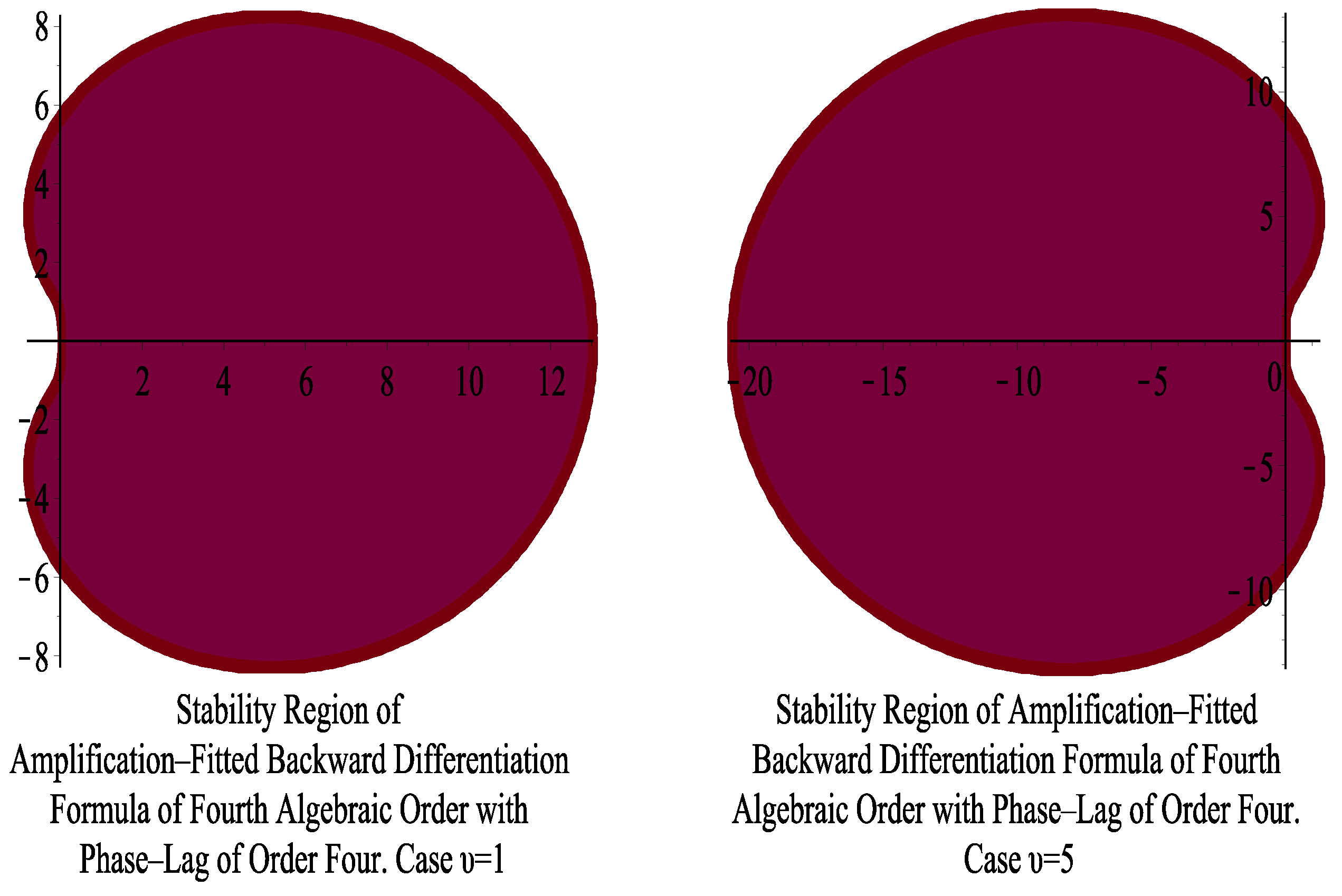
5. Amplification–Fitted Backward Differentiation Formula of Fourth Algebraic Order with Phase–Lag of Order Four

Let us consider the method (21) with:

$$\begin{array}{ccc}\hfill {\kappa }_3& =& -{\displaystyle \frac{48}{25}},{\kappa }_2={\displaystyle \frac{36}{25}}\hfill \\ \hfill {\kappa }_0& =& {\displaystyle \frac{3}{25}}.\hfill \end{array}$$

(24)

5.1. An Approach to Reducing Phase–Lag

This is the process that reduces the phase–lag

• Elimination of the Amplification–Factor.
• Using the coefficient obtained in the previous step, perform the phase–lag calculation.
• Expansion of the previously determined phase–lag via the use of Taylor series.
• Determining the system of equations that reduces the phase–lag.
• Determine the revised coefficients.

Applying the above procedure, we obtain the following:

5.2. Eliminating the Amplification Factor

Applying the direct formula for the computation of the amplification–factor (20) to the method (21) with coefficients given by (24), we obtain the following result:

$$AmplF={\displaystyle \frac{25\upsilon \varrho cos\left(4\upsilon \right)-36sin\left(2\upsilon \right)-25sin\left(4\upsilon \right)+48sin\left(3\upsilon \right)-25{\kappa }_{1}sin\left(\upsilon \right)}{400{\upsilon }^2\varrho +25{\kappa }_1-188}},$$

(25)

where the Amplification–Factor is represented by $AmplF$.

Requesting the elimination of the amplification–factor, or requesting $AmplF=0$, we obtain:

$$\varrho ={\displaystyle \frac{1}{25}}{\displaystyle \frac{25{\kappa }_{1}sin\left(\upsilon \right)+25sin\left(4\upsilon \right)+36sin\left(2\upsilon \right)-48sin\left(3\upsilon \right)}{\upsilon cos\left(4\upsilon \right)}}.$$

(26)

Applying the coefficients ${\kappa }_i,i=0,2,3$ given by (22) and the coefficient $\varrho$ obtained in (24) to the direct formula for computation of the phase–lag given by (18), we achieve the following:

$$PhErr={\displaystyle \frac{Pa{r}_3}{Pa{r}_4}},$$

(27)

where:

$$\begin{array}{ccc}\hfill Pa{r}_3& =& [24{\left(cos\left(\upsilon \right)\right)}^4+100{\left(cos\left(\upsilon \right)\right)}^3{\kappa }_1\hfill \\ & +& 48{\left(cos\left(\upsilon \right)\right)}^2-75{\kappa }_{1}cos\left(\upsilon \right)-48cos\left(\upsilon \right)-8]\upsilon \hfill \end{array}$$

(28)

$$\begin{array}{ccc}\hfill Pa{r}_4& =& 200{\left(cos\left(\upsilon \right)\right)}^4\upsilon {\kappa }_1+896{\left(cos\left(\upsilon \right)\right)}^4\upsilon \hfill \\ & -& 200{\left(cos\left(\upsilon \right)\right)}^2\upsilon {\kappa }_1+768sin\left(\upsilon \right){\left(cos\left(\upsilon \right)\right)}^2\hfill \\ & -& 896{\left(cos\left(\upsilon \right)\right)}^2\upsilon +112sin\left(\upsilon \right)cos\left(\upsilon \right)\hfill \\ & -& 100{\kappa }_{1}sin\left(\upsilon \right)+25\upsilon {\kappa }_1+112\upsilon \hfill \\ & -& 192sin\left(\upsilon \right)-800sin\left(\upsilon \right){\left(cos\left(\upsilon \right)\right)}^3,\hfill \end{array}$$

(29)

and $PhErr$ represents the phase–lag.

We may obtain the following by expanding the Formula (27) using the Taylor series:

$$\begin{array}{ccc}\hfill PhErr& =& -{\displaystyle \frac{25{\kappa }_1+16}{75{\kappa }_1}}-{\displaystyle \frac{v^2}{75{\kappa }_1}}\left(-72-{\displaystyle \frac{225{\kappa }_1}{2}}+{\displaystyle \frac{25{\kappa }_1+16}{75{\kappa }_1}}\left(-{\displaystyle \frac{550{\kappa }_1}{3}}-{\displaystyle \frac{1504}{3}}\right)\right)\hfill \\ & -& {\displaystyle \frac{v^4}{75{\kappa }_1}}[54+{\displaystyle \frac{675{\kappa }_1}{8}}+{\displaystyle \frac{25{\kappa }_1+16}{75{\kappa }_1}}\left({\displaystyle \frac{1595{\kappa }_1}{6}}+{\displaystyle \frac{10376}{15}}\right)\hfill \\ & -& {\displaystyle \frac{78125{{\kappa }_1}^2+125200{\kappa }_1+48128}{33750{{\kappa }_1}^2}}\left(-{\displaystyle \frac{550{\kappa }_1}{3}}-{\displaystyle \frac{1504}{3}}\right)]\hfill \\ & -& {\displaystyle \frac{v^6}{75{\kappa }_1}}[-{\displaystyle \frac{101}{5}}-{\displaystyle \frac{405{\kappa }_1}{16}}+{\displaystyle \frac{25{\kappa }_1+16}{75{\kappa }_1}}\hfill \\ & & \left(-{\displaystyle \frac{11945{\kappa }_1}{84}}-{\displaystyle \frac{5876}{15}}\right)-{\displaystyle \frac{78125{{\kappa }_1}^2+125200{\kappa }_1+48128}{33750{{\kappa }_1}^2}}\hfill \\ & & \left({\displaystyle \frac{1595{\kappa }_1}{6}}+{\displaystyle \frac{10376}{15}}\right)+{\displaystyle \frac{Pa{r}_5}{30375000{{\kappa }_1}^3}}\left(-{\displaystyle \frac{550{\kappa }_1}{3}}-{\displaystyle \frac{1504}{3}}\right)]+\dots .\hfill \end{array}$$

(30)

where

$$Pa{r}_5=241934375{{\kappa }_1}^3+883662000{{\kappa }_1}^2+918850560{\kappa }_1+289538048$$

(31)

The following equation is obtained by requesting that the phase–lag be minimized:

$$-{\displaystyle \frac{25{\kappa }_1+16}{75{\kappa }_1}}=0⟹{\kappa }_1=-{\displaystyle \frac{16}{25}}.$$

(32)

This innovative algorithm has the following characteristics:

$$\begin{array}{ccc}\hfill {\kappa }_3& =& -{\displaystyle \frac{48}{25}},\hfill \\ \hfill {\kappa }_2& =& {\displaystyle \frac{36}{25}},\hfill \\ \hfill {\kappa }_1& =& -{\displaystyle \frac{16}{25}},\hfill \\ \hfill {\kappa }_0& =& {\displaystyle \frac{3}{25}},\hfill \\ \hfill \varrho & =& {\displaystyle \frac{1}{25}}{\displaystyle \frac{-16sin\left(\upsilon \right)+25sin\left(4\upsilon \right)+36sin\left(2\upsilon \right)-48sin\left(3\upsilon \right)}{\upsilon cos\left(4\upsilon \right)}},\hfill \\ \hfill LTE& =& -{\displaystyle \frac{12}{125}}{h}^5\left({\mathsf{\Psi }}^{\left\{\left(5\right)\right\}}\left(t\right)-{\omega }^4{\mathsf{\Psi }}^{\prime }\left(t\right)\right)+O\left(h^6\right),\hfill \\ \hfill PhErr& =& -{\displaystyle \frac{1}{12}}{v}^6-{\displaystyle \frac{59}{96}}{v}^8+\dots ,\hfill \\ \hfill AmplF& =& 0.\hfill \end{array}$$

(33)

We mention that $\varrho$ may be expressed as a Taylor series expansion:

$$\varrho ={\displaystyle \frac{12}{25}}-{\displaystyle \frac{12{\upsilon }^4}{125}}-{\displaystyle \frac{86{\upsilon }^6}{175}}-{\displaystyle \frac{4601{\upsilon }^8}{1500}}+\dots .$$

(34)

Remark 1. 

The outcome will be identical to what was stated before if we choose 3 free parameters, such as ${\kappa }_j,j=0\left(1\right)2$.

6. Phase–Fitted and Amplification–Fitted Backward Differentiation Formula of Algebraic Order Four with the Elimination of the First Derivative of the Amplification–Factor

Let us consider the method (21) with coefficients:

$${\kappa }_3=-{\displaystyle \frac{48}{25}},{\kappa }_1=-{\displaystyle \frac{16}{25}}$$

(35)

Methodology for the Vanishing of the First Derivative of the Amplification–Factor

• We apply the Formula (20) to the specific method (35). Thus, we obtain the formula of the Amplification–Factor, let us say $AmplF$.
• We calculate the first derivative of the above formula, i.e., ${\displaystyle \frac{\partial AmplF}{\partial \upsilon }}$.
• We request the formula of the previous step to be equal to zero, i.e., ${\displaystyle \frac{\partial AmplF}{\partial \upsilon }}=0$.

Based on the above methodology, and using the Formulae (18) and (20) to determine the phase–lag, amplification–factor, we obtain the Formulae (44) and (45).

The derivative of the amplification–factor gives the following result:

$${\displaystyle \frac{\partial AmplF}{\partial \upsilon }}=-{\displaystyle \frac{1}{4}}{\displaystyle \frac{Pa{r}_{22}}{{\left(100{\upsilon }^2\varrho +25{\kappa }_2-87\right)}^2}},$$

(36)

where the formula $Pa{r}_{22}$ is in Appendix D.

Requesting the elimination of the phase–lag, the amplification–factor, and the derivative of the amplification–factor, i.e., requesting $PhErr=0$, $AmplF=0$, and ${\displaystyle \frac{\partial AmplF}{\partial \upsilon }}=0$ we obtain:

$$\begin{array}{ccc}\hfill {\kappa }_2& =& {\displaystyle \frac{Pa{r}_{23}}{Pa{r}_{24}}}\hfill \end{array}$$

(37)

$$\begin{array}{ccc}\hfill {\kappa }_0& =& {\displaystyle \frac{Pa{r}_{25}}{Pa{r}_{26}}}\hfill \end{array}$$

(38)

$$\begin{array}{ccc}\hfill \varrho & =& {\displaystyle \frac{-48sin\left(5\upsilon \right)+192sin\left(\upsilon \right)+50sin\left(6\upsilon \right)-150sin\left(2\upsilon \right)+16sin\left(3\upsilon \right)}{50\upsilon cos\left(6\upsilon \right)-150\upsilon cos\left(2\upsilon \right)+25sin\left(6\upsilon \right)-25sin\left(2\upsilon \right)}},\hfill \end{array}$$

(39)

where the formulae $Pa{r}_j,j=23\left(1\right)26$ are in Appendix E.

The following is the result of applying the Taylor series to the previously stated formulae:

$$\begin{array}{ccc}\hfill {\kappa }_0& =& {\displaystyle \frac{3}{25}}-{\displaystyle \frac{18{\upsilon }^2}{1375}}-{\displaystyle \frac{7641{\upsilon }^4}{1058750}}-{\displaystyle \frac{1014751{\upsilon }^6}{116462500}}\hfill \\ & -& {\displaystyle \frac{5154660383{\upsilon }^8}{358704500000}}-{\displaystyle \frac{10843023989719{\upsilon }^{10}}{512947435000000}}\hfill \\ & -& {\displaystyle \frac{615072100312758827{\upsilon }^{12}}{21328354347300000000}}+\cdots \hfill \end{array}$$

(40)

$$\begin{array}{ccc}\hfill {\kappa }_2& =& {\displaystyle \frac{36}{25}}+{\displaystyle \frac{18{\upsilon }^2}{1375}}-{\displaystyle \frac{75519{\upsilon }^4}{1058750}}+{\displaystyle \frac{11556491{\upsilon }^6}{116462500}}\hfill \\ & +& {\displaystyle \frac{33843209503{\upsilon }^8}{358704500000}}+{\displaystyle \frac{61617963722379{\upsilon }^{10}}{512947435000000}}\hfill \\ & +& {\displaystyle \frac{3295535984888285107{\upsilon }^{12}}{21328354347300000000}}+\cdots \hfill \end{array}$$

(41)

$$\begin{array}{ccc}\hfill \varrho & =& {\displaystyle \frac{12}{25}}+{\displaystyle \frac{36{\upsilon }^2}{1375}}-{\displaystyle \frac{24699{\upsilon }^4}{529375}}-{\displaystyle \frac{4594589{\upsilon }^6}{58231250}}\hfill \\ & -& {\displaystyle \frac{19274549037{\upsilon }^8}{179352250000}}-{\displaystyle \frac{326113634777069{\upsilon }^{10}}{2308263457500000}}\hfill \\ & -& {\displaystyle \frac{1967731067173147153{\upsilon }^{12}}{10664177173650000000}}+\cdots \hfill \end{array}$$

(42)

This novel algorithm has the following features:

$$\begin{array}{ccc}\hfill {\kappa }_2& \mathrm{is}\mathrm{given}\mathrm{by}& \left(37\right)\hfill \\ \hfill {\kappa }_0& \mathrm{is}\mathrm{given}\mathrm{by}& \left(38\right)\hfill \\ \hfill \varrho & \mathrm{is}\mathrm{given}\mathrm{by}& \left(39\right)\hfill \\ \hfill LTE& =& -{\displaystyle \frac{108}{1375}}{h}^4\left({\omega }^4{\mathsf{\Psi }}^{\left\{\left(4\right)\right\}}\left(t\right)+{\omega }^2{\mathsf{\Psi }}^{″}\left(t\right)\right)+O\left(h^5\right),\hfill \\ \hfill PhErr& =& 0\hfill \\ \hfill AmplF& =& 0\hfill \\ \hfill {\displaystyle \frac{\partial AmplF}{\partial \upsilon }}& =& 0.\hfill \end{array}$$

(43)

7. Phase–Fitted and Amplification–Fitted Backward Differentiation Formula of Algebraic Order Four with the Elimination of the First Derivative of the Phase–Lag

Let us consider the method (21) with coefficients given by (35).

Methodology for the Vanishing of the First Derivative of the Phase–Lag

• We apply the Formula (18) to the specific method (35). Thus, we obtain the formula of the phase–lag, let say $PhErr$.
• We calculate the first derivative of the above formula, i.e., ${\displaystyle \frac{\partial PhErr}{\partial \upsilon }}$.
• We request the formula of the previous step to be equal to zero, i.e., ${\displaystyle \frac{\partial PhErr}{\partial \upsilon }}=0$.

Based on the above methodology, and using the Formulae (18) and (20) to determine the phase–lag, amplification–factor, and the derivative of the phase–lag, yields the following result:

$$\begin{array}{ccc}\hfill PhErr& =& {\displaystyle \frac{Pa{r}_{15}}{-48-100\varrho +100{\kappa }_2}}\hfill \end{array}$$

(44)

$$\begin{array}{ccc}\hfill AmplF& =& {\displaystyle \frac{Pa{r}_{16}}{400{\upsilon }^2\varrho +100{\kappa }_2-348}}\hfill \end{array}$$

(45)

$$\begin{array}{ccc}\hfill {\displaystyle \frac{\partial PhErr}{\partial \upsilon }}& =& {\displaystyle \frac{Pa{r}_{17}}{-48-100\varrho +100{\kappa }_2}},\hfill \end{array}$$

(46)

where

$$\begin{array}{ccc}\hfill Pa{r}_{15}& =& 25\upsilon \varrho sin\left(4\upsilon \right)+25cos\left(4\upsilon \right)-48cos\left(3\upsilon \right)\hfill \\ & -& 16cos\left(\upsilon \right)+25{\kappa }_{2}cos\left(2\upsilon \right)+25{\kappa }_0\hfill \end{array}$$

(47)

$$\begin{array}{ccc}\hfill Pa{r}_{16}& =& 25\upsilon \varrho cos\left(4\upsilon \right)-25{\kappa }_{2}sin\left(2\upsilon \right)+16sin\left(\upsilon \right)\hfill \\ & -& 25sin\left(4\upsilon \right)+48sin\left(3\upsilon \right)\hfill \end{array}$$

(48)

$$\begin{array}{ccc}\hfill Pa{r}_{17}& =& 100\upsilon \varrho cos\left(4\upsilon \right)-50{\kappa }_{2}sin\left(2\upsilon \right)+25\varrho sin\left(4\upsilon \right)\hfill \\ & +& 16sin\left(\upsilon \right)-100sin\left(4\upsilon \right)+144sin\left(3\upsilon \right).\hfill \end{array}$$

(49)

Requesting the elimination of the phase–lag, the amplification–factor and the derivative of the phase–lag, i.e., requesting $PhErr=0$, $AmplF=0$, and ${\displaystyle \frac{\partial PhErr}{\partial \upsilon }}=0$ we obtain:

$$\begin{array}{ccc}\hfill {\kappa }_2& =& {\displaystyle \frac{Pa{r}_{18}}{Pa{r}_{19}}}\hfill \end{array}$$

(50)

$$\begin{array}{ccc}\hfill {\kappa }_0& =& {\displaystyle \frac{Pa{r}_{20}}{Pa{r}_{21}}}\hfill \end{array}$$

(51)

$$\begin{array}{ccc}\hfill \varrho & =& {\displaystyle \frac{50sin\left(4\upsilon \right)-48sin\left(3\upsilon \right)+16sin\left(\upsilon \right)}{50\upsilon cos\left(4\upsilon \right)+25sin\left(4\upsilon \right)}},\hfill \end{array}$$

(52)

where the formulae $Pa{r}_k,k=18\left(1\right)21$ are in Appendix C.

The following is the result of applying the Taylor series to the previously stated formulae:

$$\begin{array}{ccc}\hfill {\kappa }_0& =& {\displaystyle \frac{3}{25}}+{\displaystyle \frac{6}{125}}{\upsilon }^4+{\displaystyle \frac{431}{2625}}{\upsilon }^6+{\displaystyle \frac{475163}{945000}}{\upsilon }^8\hfill \\ & +& {\displaystyle \frac{286895963}{187110000}}{\upsilon }^{10}+{\displaystyle \frac{14344436937211}{3064861800000}}{\upsilon }^{12}+\cdots \hfill \end{array}$$

(53)

$$\begin{array}{ccc}\hfill {\kappa }_2& =& {\displaystyle \frac{36}{25}}-{\displaystyle \frac{6}{125}}{\upsilon }^4+{\displaystyle \frac{149}{525}}{\upsilon }^6+{\displaystyle \frac{754417}{945000}}{\upsilon }^8\hfill \\ & +& {\displaystyle \frac{456321589}{187110000}}{\upsilon }^{10}+{\displaystyle \frac{22821441228569}{3064861800000}}{\upsilon }^{12}+\cdots \hfill \end{array}$$

(54)

$$\begin{array}{ccc}\hfill \varrho & =& {\displaystyle \frac{12}{25}}-{\displaystyle \frac{24}{125}}{\upsilon }^4-{\displaystyle \frac{1648}{2625}}{\upsilon }^6-{\displaystyle \frac{455713}{236250}}{\upsilon }^8\hfill \\ & -& {\displaystyle \frac{3939379}{668250}}{\upsilon }^{10}-{\displaystyle \frac{13795647774791}{766215450000}}{\upsilon }^{12}+\cdots \hfill \end{array}$$

(55)

This novel algorithm has the following features:

$$\begin{array}{ccc}\hfill {\kappa }_2& \mathrm{is}\mathrm{given}\mathrm{by}& \left(50\right)\hfill \\ \hfill {\kappa }_0& \mathrm{is}\mathrm{given}\mathrm{by}& \left(51\right)\hfill \\ \hfill \varrho & \mathrm{is}\mathrm{given}\mathrm{by}& \left(52\right)\hfill \\ \hfill LTE& =& -{\displaystyle \frac{12}{125}}{h}^5\left({\mathsf{\Psi }}^{\left\{\left(5\right)\right\}}\left(t\right)-{\omega }^4{\mathsf{\Psi }}^{\prime }\left(t\right)\right)+O\left(h^6\right),\hfill \\ \hfill PhErr& =& 0\hfill \\ \hfill AmplF& =& 0\hfill \\ \hfill {\displaystyle \frac{\partial PhErr}{\partial \upsilon }}& =& 0.\hfill \end{array}$$

(56)

where $PhErr$ is the phase–lag, $AmplF$ is the amplification–factor, and ${\displaystyle \frac{\partial PhErr}{\partial \upsilon }}$ is the first derivative of the phase–lag.

8. Amplification–Fitted Backward Differentiation Formula of Second Algebraic Order with Phase–Lag of Order Six

Let us consider the method (21) with all the coefficients free.

Following the algorithm given in Section 5.1, we have:

Eliminating the Amplification Factor

Applying the direct formula for the computation of the amplification–factor (20) to the method (21), we obtain the following result:

$$AmplF={\displaystyle \frac{sin\left(4\upsilon \right)+{\kappa }_{1}sin\left(\upsilon \right)+{\kappa }_{2}sin\left(2\upsilon \right)+{\kappa }_{3}sin\left(3\upsilon \right)-\upsilon \varrho cos\left(4\upsilon \right)}{-16{\upsilon }^2\varrho -{\kappa }_1-4{\kappa }_2-9{\kappa }_3-4}},$$

(57)

Requesting the elimination of the amplification–factor, or requesting $AmplF=0$, we obtain:

$$\varrho ={\displaystyle \frac{{\kappa }_{1}sin\left(\upsilon \right)+{\kappa }_{2}sin\left(2\upsilon \right)+{\kappa }_{3}sin\left(3\upsilon \right)+sin\left(4\upsilon \right)}{\upsilon cos\left(4\upsilon \right)}}.$$

(58)

Applying the coefficient $\varrho$ obtained in (57) to the direct formula for computation of the phase–lag given by (18), we achieve the following:

$$PhErr={\displaystyle \frac{Pa{r}_6}{Pa{r}_7}},$$

(59)

where:

$$\begin{array}{ccc}\hfill Pa{r}_6& =& [8{\left(cos\left(\upsilon \right)\right)}^4{\kappa }_0+4{\left(cos\left(\upsilon \right)\right)}^3{\kappa }_1-8{\left(cos\left(\upsilon \right)\right)}^2{\kappa }_0\hfill \\ & +& 2{\left(cos\left(\upsilon \right)\right)}^2{\kappa }_2-3{\kappa }_{1}cos\left(\upsilon \right)\hfill \\ & +& {\kappa }_{3}cos\left(\upsilon \right)+{\kappa }_0-{\kappa }_2+1]\upsilon \hfill \end{array}$$

(60)

$$\begin{array}{ccc}\hfill Pa{r}_7& =& 8{\left(cos\left(\upsilon \right)\right)}^4\upsilon {\kappa }_1+32{\left(cos\left(\upsilon \right)\right)}^4\upsilon {\kappa }_2+72{\left(cos\left(\upsilon \right)\right)}^4\upsilon {\kappa }_3\hfill \\ & +& 128{\left(cos\left(\upsilon \right)\right)}^4\upsilon -32sin\left(\upsilon \right){\left(cos\left(\upsilon \right)\right)}^3-16{\left(cos\left(\upsilon \right)\right)}^{2}sin\left(\upsilon \right){\kappa }_3\hfill \\ & -& 8{\left(cos\left(\upsilon \right)\right)}^2\upsilon {\kappa }_1-32{\left(cos\left(\upsilon \right)\right)}^2\upsilon {\kappa }_2-72{\left(cos\left(\upsilon \right)\right)}^2\upsilon {\kappa }_3\hfill \\ & -& 8{\kappa }_{2}sin\left(\upsilon \right)cos\left(\upsilon \right)+16sin\left(\upsilon \right)cos\left(\upsilon \right)-4{\kappa }_{1}sin\left(\upsilon \right)\hfill \\ & +& 4sin\left(\upsilon \right){\kappa }_3+\upsilon {\kappa }_1+4\upsilon {\kappa }_2+9\upsilon {\kappa }_3+16\upsilon -128{\left(cos\left(\upsilon \right)\right)}^2\upsilon .\hfill \end{array}$$

(61)

We may obtain the following by expanding the Formula (59) using the Taylor series:

$$\begin{array}{ccc}\hfill PhErr& =& Pa{r}_8+Pa{r}_9{\upsilon }^2+Pa{r}_{10}{\upsilon }^4+Pa{r}_{11}{\upsilon }^6+Pa{r}_{12}{\upsilon }^8+\dots ,\hfill \end{array}$$

(62)

where $Pa{r}_i,i=8\left(1\right)12$ are given in the Appendix B.

The following system of equations is obtained by requesting that the phase–lag be minimized:

$$\begin{array}{ccc}\hfill Pa{r}_8& =& 0\hfill \\ \hfill Pa{r}_9& =& 0\hfill \\ \hfill Pa{r}_{10}& =& 0\hfill \\ \hfill Pa{r}_{11}& =& 0\hfill \\ \hfill Pa{r}_{12}& =& 0\hfill \end{array}$$

(63)

The solution of the above system of equations is given by:

$$\begin{array}{ccc}\hfill {\kappa }_0& =& {\displaystyle \frac{1}{35}},{\kappa }_1=-{\displaystyle \frac{8}{35}},\hfill \\ \hfill {\kappa }_2& =& {\displaystyle \frac{4}{5}},{\kappa }_3=-{\displaystyle \frac{8}{5}}.\hfill \end{array}$$

(64)

This innovative algorithm has the following characteristics:

$$\begin{array}{ccc}\hfill {\kappa }_3& =& -{\displaystyle \frac{8}{5}},\hfill \\ \hfill {\kappa }_2& =& {\displaystyle \frac{4}{5}},\hfill \\ \hfill {\kappa }_1& =& -{\displaystyle \frac{8}{35}},\hfill \\ \hfill {\kappa }_0& =& {\displaystyle \frac{1}{35}},\hfill \\ \hfill \varrho & =& {\displaystyle \frac{1}{35}}{\displaystyle \frac{-8sin\left(\upsilon \right)+28sin\left(2\upsilon \right)-56sin\left(3\upsilon \right)+35sin\left(4\upsilon \right)}{\upsilon cos\left(4\upsilon \right)}},\hfill \\ \hfill LTE& =& -{\displaystyle \frac{8}{105}}{h}^3\left({\mathsf{\Psi }}^{\left\{\left(3\right)\right\}}\left(t\right)-{\omega }^2{\mathsf{\Psi }}^{\prime }\left(t\right)\right)+O\left(h^4\right),\hfill \\ \hfill PhErr& =& -{\displaystyle \frac{1}{160}}{v}^8+{\displaystyle \frac{39}{800}}{v}^{10}+\dots ,\hfill \\ \hfill AmplF& =& 0.\hfill \end{array}$$

(65)

We mention that $\varrho$ may be expressed as a Taylor series expansion:

$$\varrho ={\displaystyle \frac{4}{7}}+{\displaystyle \frac{8}{105}}{\upsilon }^2+{\displaystyle \frac{2}{105}}{\upsilon }^4+{\displaystyle \frac{151}{11025}}{\upsilon }^6+{\displaystyle \frac{1517}{31752}}{\upsilon }^8+\dots .$$

(66)

9. Phase–Fitted and Amplification–Fitted Backward Differentiation Formula of Algebraic Order Four

Let us consider the method (21) with:

$$\begin{array}{ccc}\hfill {\kappa }_3& =& -{\displaystyle \frac{48}{25}},{\kappa }_1=-{\displaystyle \frac{16}{25}}\hfill \\ \hfill {\kappa }_0& =& {\displaystyle \frac{3}{25}}.\hfill \end{array}$$

(67)

Using the Formulae (18) and (20) to determine the phase–lag and amplification–factor, respectively, yields the following result:

$$\begin{array}{ccc}\hfill PhErr& =& {\displaystyle \frac{Pa{r}_{13}}{-48-100\varrho +100{\kappa }_2}}\hfill \end{array}$$

(68)

$$\begin{array}{ccc}\hfill AmplF& =& {\displaystyle \frac{Pa{r}_{14}}{400{\upsilon }^2\varrho +100{\kappa }_2-348}},\hfill \end{array}$$

(69)

where

$$\begin{array}{ccc}\hfill Pa{r}_{13}& =& 25\upsilon \varrho sin\left(4\upsilon \right)+25{\kappa }_{2}cos\left(2\upsilon \right)+25cos\left(4\upsilon \right)\hfill \\ & -& 16cos\left(\upsilon \right)-48cos\left(3\upsilon \right)+3\hfill \end{array}$$

(70)

$$\begin{array}{ccc}\hfill Pa{r}_{14}& =& 25\upsilon \varrho cos\left(4\upsilon \right)-25{\kappa }_{2}sin\left(2\upsilon \right)-25sin\left(4\upsilon \right)\hfill \\ & +& 16sin\left(\upsilon \right)+48sin\left(3\upsilon \right).\hfill \end{array}$$

(71)

and $AmplF$ stands for the Amplification Factor, while $PhErr$ is the phase–lag.

Requesting the elimination of the phase–lag and the amplification–factor, i.e., requesting $PhErr=0$ and $AmplF=0$, we obtain:

$$\begin{array}{ccc}\hfill {\kappa }_2& =& {\displaystyle \frac{1}{25}}{\displaystyle \frac{-25-3cos\left(4\upsilon \right)+48cos\left(\upsilon \right)+16cos\left(3\upsilon \right)}{cos\left(2\upsilon \right)}}\hfill \end{array}$$

(72)

$$\begin{array}{ccc}\hfill \varrho & =& {\displaystyle \frac{1}{25}}{\displaystyle \frac{22sin\left(2\upsilon \right)-32sin\left(\upsilon \right)}{cos\left(2\upsilon \right)\upsilon }}.\hfill \end{array}$$

(73)

The following is the result of applying the Taylor series to the previously stated formulae:

$$\begin{array}{ccc}\hfill {\kappa }_2& =& {\displaystyle \frac{36}{25}}+{\displaystyle \frac{4}{25}}{\upsilon }^6+{\displaystyle \frac{11}{50}}{\upsilon }^8+{\displaystyle \frac{179}{500}}{\upsilon }^{10}+{\displaystyle \frac{219259}{378000}}{\upsilon }^{12}+\cdots \hfill \end{array}$$

(74)

$$\begin{array}{ccc}\hfill \varrho & =& {\displaystyle \frac{12}{25}}-{\displaystyle \frac{12}{125}}{\upsilon }^4-{\displaystyle \frac{6}{35}}{\upsilon }^6-{\displaystyle \frac{421}{1500}}{\upsilon }^8-{\displaystyle \frac{63131}{138600}}{\upsilon }^{10}-{\displaystyle \frac{1344073}{1820000}}{\upsilon }^{12}+\cdots \hfill \end{array}$$

(75)

This innovative algorithm has the following characteristics:

$$\begin{array}{ccc}\hfill {\kappa }_3& =& -{\displaystyle \frac{48}{25}},\hfill \\ \hfill {\kappa }_2& \mathrm{see}& \left(72\right),\hfill \\ \hfill {\kappa }_1& =& -{\displaystyle \frac{16}{25}},\hfill \\ \hfill {\kappa }_0& =& {\displaystyle \frac{3}{25}},\hfill \\ \hfill \varrho & \mathrm{see}& \left(73\right),\hfill \\ \hfill LTE& =& -{\displaystyle \frac{12}{125}}{h}^5\left({\mathsf{\Psi }}^{\left\{\left(5\right)\right\}}\left(t\right)-{\omega }^4{\mathsf{\Psi }}^{\prime }\left(t\right)\right)+O\left(h^6\right),\hfill \\ \hfill PhErr& =& 0,\hfill \\ \hfill AmplF& =& 0.\hfill \end{array}$$

(76)

10. Phase–Fitted and Amplification–Fitted Backward Differentiation Formula of Algebraic Order Four with the Elimination of the First Derivative of the Phase–Lag and the First Derivative of the Amplification–Factor

Let us consider the method (21) with:

$${\kappa }_3=-{\displaystyle \frac{48}{25}}$$

(77)

Methodology for the Vanishing of the First Derivative of the Phase–Lag and the First Derivative of the Amplification–Factor

• We apply the Formula (18) to the specific method (78). Thus, we obtain the formula of the Phase–Lag, let say $PhErr$.
• We calculate the first derivative of the above formula, i.e., ${\displaystyle \frac{\partial PhErr}{\partial \upsilon }}$.
• We apply the Formula (20) to the specific method (78). Thus, we obtain the formula of the Amplification–Factor, let say $AmplF$.
• We calculate the first derivative of the above formula, i.e., ${\displaystyle \frac{\partial AmplF}{\partial \upsilon }}$.
• We request the formulae of the previous steps to be equal to zero, i.e., ${\displaystyle \frac{\partial PhErr}{\partial \upsilon }}=0$, and ${\displaystyle \frac{\partial AmplF}{\partial \upsilon }}=0$.

Based on the above methodology, and using the Formulae (18) and (20) to determine the phase–lag, amplification–factor, we obtain:

$$\begin{array}{ccc}\hfill PhErr& =& {\displaystyle \frac{Pa{r}_{27}}{-32-100\varrho +25{\kappa }_1+100{\kappa }_2}}\hfill \end{array}$$

(78)

$$\begin{array}{ccc}\hfill AmplF& =& {\displaystyle \frac{Pa{r}_{28}}{400{\upsilon }^2\varrho +25{\kappa }_1+100{\kappa }_2-332}}\hfill \end{array}$$

(79)

$$\begin{array}{ccc}\hfill {\displaystyle \frac{\partial PhErr}{\partial \upsilon }}& =& {\displaystyle \frac{Pa{r}_{29}}{-32-100\varrho +25{\kappa }_1+100{\kappa }_2}}\hfill \end{array}$$

(80)

$$\begin{array}{ccc}\hfill {\displaystyle \frac{\partial AmplF}{\partial \upsilon }}& =& {\displaystyle \frac{Pa{r}_{30}}{Pa{r}_{31}}},\hfill \end{array}$$

(81)

where the formulae $Pa{r}_q,q=27\left(1\right)31$ are in Appendix F.

Requesting the elimination of the phase–lag, the amplification–factor, the derivative of the phase–lag, and the derivative of the amplification–factor, i.e., requesting $PhErr=0$, $AmplF=0$, ${\displaystyle \frac{\partial PhErr}{\partial \upsilon }}=0$, and ${\displaystyle \frac{\partial AmplF}{\partial \upsilon }}=0$ we obtain:

$$\begin{array}{ccc}\hfill {\kappa }_2& =& {\displaystyle \frac{Pa{r}_{32}}{100cos\left(2\upsilon \right)\upsilon -50cos\left(4\upsilon \right)\upsilon +25sin\left(2\upsilon \right)-25sin\left(4\upsilon \right)}}\hfill \end{array}$$

(82)

$$\begin{array}{ccc}\hfill {\kappa }_1& =& {\displaystyle \frac{Pa{r}_{33}}{100cos\left(2\upsilon \right)\upsilon -50cos\left(4\upsilon \right)\upsilon +25sin\left(2\upsilon \right)-25sin\left(4\upsilon \right)}}\hfill \end{array}$$

(83)

$$\begin{array}{ccc}\hfill {\kappa }_0& =& {\displaystyle \frac{Pa{r}_{34}}{100cos\left(2\upsilon \right)\upsilon -50cos\left(4\upsilon \right)\upsilon +25sin\left(2\upsilon \right)-25sin\left(4\upsilon \right)}}\hfill \end{array}$$

(84)

$$\begin{array}{ccc}\hfill \varrho & =& {\displaystyle \frac{-50sin\left(4\upsilon \right)+100sin\left(2\upsilon \right)+48sin\left(3\upsilon \right)-144sin\left(\upsilon \right)}{100cos\left(2\upsilon \right)\upsilon -50cos\left(4\upsilon \right)\upsilon +25sin\left(2\upsilon \right)-25sin\left(4\upsilon \right)}},\hfill \end{array}$$

(85)

where the formulae $Pa{r}_i,i=32\left(1\right)34$ are in Appendix G.

This novel algorithm has the following features:

$$\begin{array}{ccc}\hfill {\kappa }_2& \mathrm{is}\mathrm{given}\mathrm{by}& \left(82\right)\hfill \\ \hfill {\kappa }_2& \mathrm{is}\mathrm{given}\mathrm{by}& \left(83\right)\hfill \\ \hfill {\kappa }_0& \mathrm{is}\mathrm{given}\mathrm{by}& \left(84\right)\hfill \\ \hfill \varrho & \mathrm{is}\mathrm{given}\mathrm{by}& \left(85\right)\hfill \\ \hfill LTE& =& -{\displaystyle \frac{12}{125}}{h}^5\left({\mathsf{\Psi }}^{\left\{\left(5\right)\right\}}\left(t\right)+2{\omega }^2{\mathsf{\Psi }}^{\left\{\left(3\right)\right\}}\left(t\right)+{\omega }^4{\mathsf{\Psi }}^{\prime }\left(t\right)\right)+O\left(h^6\right),\hfill \\ \hfill PhErr& =& 0\hfill \\ \hfill AmplF& =& 0\hfill \\ \hfill {\displaystyle \frac{\partial AmplF}{\partial \upsilon }}& =& 0.\hfill \end{array}$$

(86)

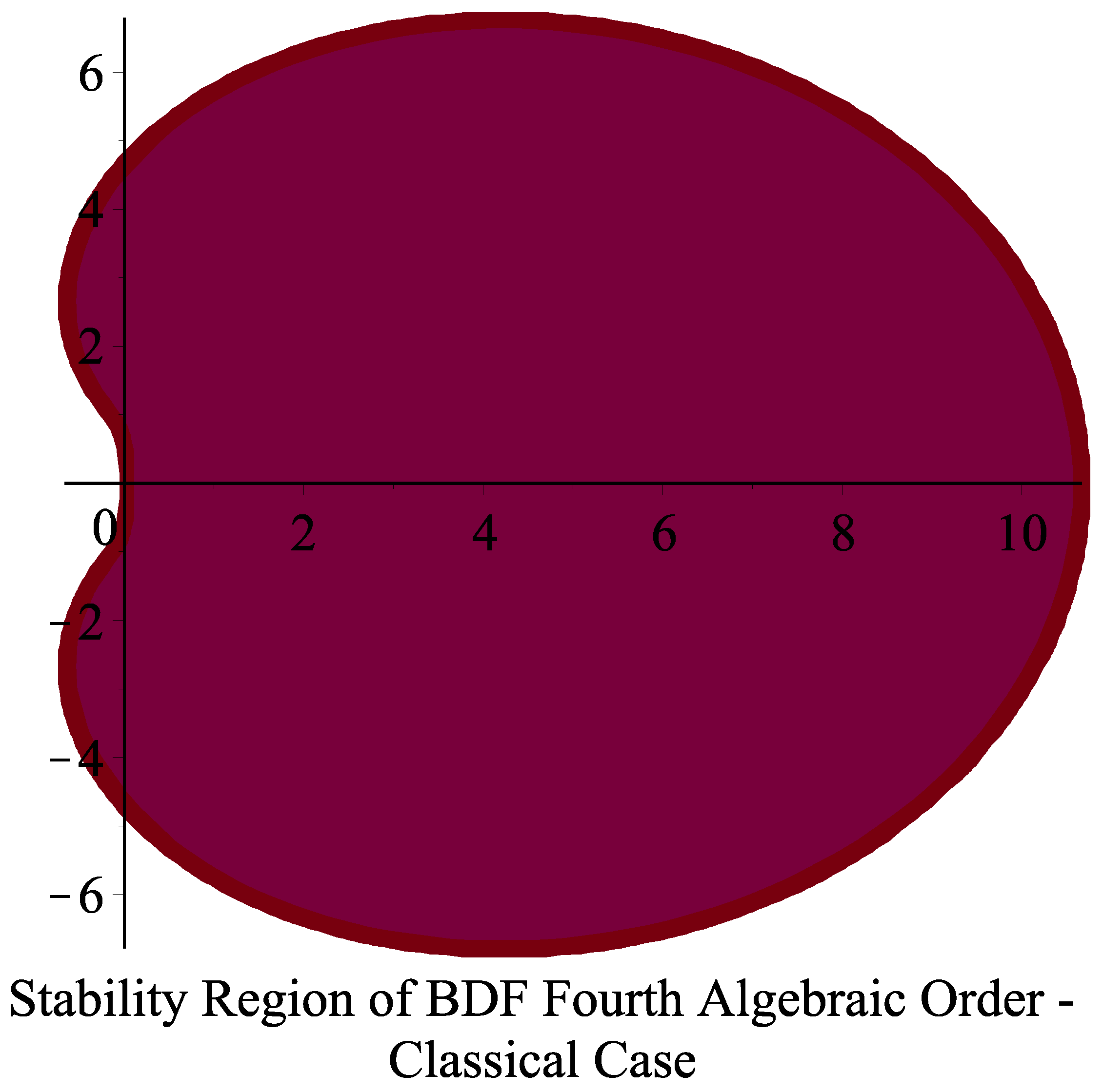
11. Stability Analysis

The Backward Differentiation Formula which studied in this paper has the general form:

$${\mathsf{\Psi }}_{n+2}+{\mathsf{\Lambda }}_3{\mathsf{\Psi }}_{n+1}+{\mathsf{\Lambda }}_2{\mathsf{\Psi }}_n+{\mathsf{\Lambda }}_1{\mathsf{\Psi }}_{n-1}+{\mathsf{\Lambda }}_0{\mathsf{\Psi }}_{n-2}=h\mathsf{\Omega }{\mathsf{\Xi }}_{n+2}.$$

(87)

where ${\mathsf{\Xi }}_{n+2}={\mathsf{\Psi }}_{n+2}^{\prime }$.

The method (87) encompasses the methods that were created in Section 4, Section 5, Section 6, Section 7, Section 8, Section 9 and Section 10, namely the methods (22), (33), (43), (56), (65), (76), and (86).

Based on the scalar test equation:

$${\mathsf{\Psi }}^{\prime }=\lambda \mathsf{\Psi }\mathrm{where}\lambda \in \mathcal{C},$$

(88)

we can obtain the following difference equation by implementing the scheme (A21).

$${\mathsf{\Gamma }}_4{\mathsf{\Psi }}_{n+2}+{\mathsf{\Gamma }}_3{\mathsf{\Psi }}_{n+1}+{\mathsf{\Gamma }}_2{\mathsf{\Psi }}_n+{\mathsf{\Gamma }}_1{\mathsf{\Psi }}_{n-1}+{\mathsf{\Gamma }}_0{\mathsf{\Psi }}_{n-2}=0.$$

(89)

where

$$\begin{array}{c}\hfill {\mathsf{\Gamma }}_4\left(Z\right)=1-\mathsf{\Omega }Z,{\mathsf{\Gamma }}_3\left(Z\right)={\mathsf{\Lambda }}_3,{\mathsf{\Gamma }}_2\left(Z\right)={\mathsf{\Lambda }}_2,{\mathsf{\Gamma }}_1\left(V\right)={\mathsf{\Lambda }}_1,{\mathsf{\Gamma }}_0\left(V\right)={\mathsf{\Lambda }}_0.\end{array}$$

(90)

and $Z=\lambda h$

The characteristic equation of (A22) is given by

$${\mathsf{\Gamma }}_4\left(Z\right)q^4+{\mathsf{\Gamma }}_3\left(Z\right)q^3+{\mathsf{\Gamma }}_2\left(Z\right)q^2+{\mathsf{\Gamma }}_1\left(Z\right)q+{\mathsf{\Gamma }}_0\left(Z\right)=0.$$

(91)

It is possible to determine the stability regions for $\zeta \in [0,2\pi ]$ by solving the above Equation (91) in Z and replacing q with $q=exp\left(i\zeta \right)$, where $i=\sqrt{-1}$. Figure 1 illustrates the stability of the Backward Differentiation Formula stated in Section 4 Classical Case with constant coefficients. The stability regions of the algorithms derived from Section 5, Section 6, Section 8, Section 9 and Section 10 are shown in Figure 2, Figure 3, Figure 4, Figure 5, Figure 6, Figure 7, Figure 8 and Figure 9. For these cases we present the stability regions for $v=1$, $v=5$, $v=10$, and $v=100$.

12. Numerical Results

For the below mentioned problems, and in the case that we have second order differential equations or systems of second order differential equations, we analyze them to systems of first order differential equations using the techniques presented in the literature (for example see the book [33], chapter 7). For all the examples which are presented below, we use a step length of ${\displaystyle \frac{1}{2^q}}$ for several values of q.

12.1. Problem of Stiefel and Bettis

The following nearly periodic orbit problem was studied by Stiefel and Bettis [31] and is taken into account here:

$$\begin{array}{ccc}\hfill {\mathsf{\Psi }}_1^{″}\left(t\right)& =& -{\mathsf{\Psi }}_1\left(t\right)+0.001cos\left(t\right),{\mathsf{\Psi }}_1\left(0\right)=1,{\mathsf{\Psi }}_1^{\prime }\left(0\right)=0,\hfill \\ \hfill {\mathsf{\Psi }}_2^{″}\left(t\right)& =& -{\mathsf{\Psi }}_2\left(t\right)+0.001sin\left(t\right),{\mathsf{\Psi }}_2\left(0\right)=0,{\mathsf{\Psi }}_2^{\prime }\left(0\right)=0.9995.\hfill \end{array}$$

(92)

The exact solution is

$$\begin{array}{c}\hfill {\mathsf{\Psi }}_1\left(t\right)=cos\left(t\right)+0.0005tsin\left(t\right),\\ \hfill {\mathsf{\Psi }}_2\left(t\right)=sin\left(t\right)-0.0005tcos\left(t\right).\end{array}$$

(93)

For this problem, we use $\omega =1$.

The problem (92) has numerical solutions for $0\le t\le$ 100,000 that have been determined by using the corresponding methods:

• The Backward Differentiation Formula presented in Section 4 (Classical Case), which is mentioned as Comput. Algorith. I
• The Runge–Kutta Dormand and Prince fourth order method [14], which is mentioned as Comput. Algorith. II
• The Runge–Kutta Dormand and Prince fifth order method [14], which is mentioned as Comput. Algorith. III
• The Runge–Kutta Fehlberg fourth order method [34], which is mentioned as Comput. Algorith. IV
• The Runge–Kutta Fehlberg fifth order method [34], which is mentioned as Comput. Algorith. V
• The Runge–Kutta Cash and Karp fifth order method [35], which is mentioned as Comput. Algorith. VI
• The Amplification–Fitted Backward Differentiation Formula with Phase–Lag of order 4, which is developed in Section 5, and which is mentioned as Comput. Algorith. VII
• The Phase–Fitted and Amplification–Fitted Backward Differentiation Formula with vanished the first derivative of the amplification–factor which is developed in Section 6, and which is mentioned as Comput. Algorith. VIII
• The Phase–Fitted and Amplification–Fitted Backward Differentiation Formula with vanished the first derivative of the phase–lag which is developed in Section 7, and which is mentioned as Comput. Algorith. IX
• The Amplification–Fitted Backward Differentiation Formula with Phase–Lag of order 6, which is developed in Section 8, and which is mentioned as Comput. Algorith. X
• The Phase–Fitted and Amplification–Fitted Backward Differentiation Formula which is developed in Section 9, and which is mentioned as Comput. Algorith. XI
• The Phase–Fitted and Amplification–Fitted Backward Differentiation Formula with vanished the first derivative of the phase–lag and vanished the first derivative of the amplification–factor which is developed in Section 10, which is mentioned as Comput. Algorith. XII

Figure 8 displays the maximum absolute error of the solutions derived from the Stiefel and Bettis [31] problem using each of the numerical techniques previously described.

Figure 8 provides the data that enable us to see the following:

• Comput. Algorith. X is more efficient than Comput. Algorith. III
• Comput. Algorith. I is more efficient than Comput. Algorith. V
• Comput. Algorith. VI has the same, generally, behavior with Comput. Algorith. I
• Comput. Algorith. V is more efficient than Comput. Algorith. I
• Comput. Algorith. IV has the same, generally, behavior with Comput. Algorith. V
• Comput. Algorith. II is more efficient than Comput. Algorith. V
• Comput. Algorith. VII is more efficient than Comput. Algorith. II
• Comput. Algorith. VIII gives mixed results. For big step sizes is more efficient than Comput. Algorith. VII. For small step sizes is less efficient than Comput. Algorith. VII.
• Comput. Algorith. XI has the same, generally, behavior with Comput. Algorith. IX
• Comput. Algorith. XI is more efficient than Comput. Algorith. VIII
• Finally, Comput. Algorith. XII, is the most efficient one.

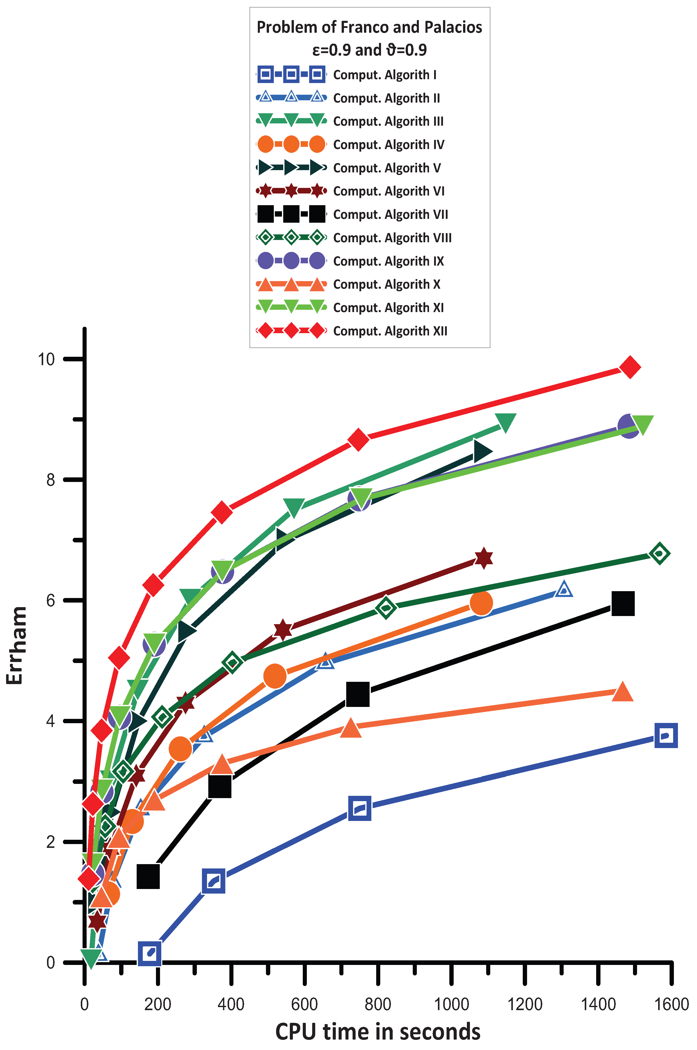
12.2. Problem of Franco and Palacios [32]

The following problem was examined by Franco and Palacios [32] and is taken into account here:

$$\begin{array}{ccc}\hfill {\mathsf{\Psi }}_1^{″}\left(t\right)& =& -{\mathsf{\Psi }}_1\left(t\right)+\epsilon cos\left(\vartheta t\right),{\mathsf{\Psi }}_1\left(0\right)=1,{\mathsf{\Psi }}_1^{\prime }\left(0\right)=0,\hfill \\ \hfill {\mathsf{\Psi }}_2^{″}\left(t\right)& =& -{\mathsf{\Psi }}_2\left(t\right)+\epsilon sin\left(\vartheta t\right),{\mathsf{\Psi }}_2\left(0\right)=0,{\mathsf{\Psi }}_2^{\prime }\left(0\right)=1.\hfill \end{array}$$

(94)

The exact solution is

$$\begin{array}{c}\hfill {\mathsf{\Psi }}_1\left(t\right)={\displaystyle \frac{1-\epsilon -{\vartheta }^2}{1-{\vartheta }^2}}cos\left(t\right)+{\displaystyle \frac{\epsilon }{1-{\vartheta }^2}}cos\left(\vartheta t\right),\\ \hfill {\mathsf{\Psi }}_2\left(t\right)={\displaystyle \frac{1-\epsilon \vartheta -{\vartheta }^2}{1-{\vartheta }^2}}sin\left(t\right)+{\displaystyle \frac{\epsilon }{1-{\vartheta }^2}}sin\left(\vartheta t\right),\end{array}$$

(95)

where $\epsilon =0.9$ and $\vartheta =0.9$. For this problem, we use $\omega =max\left(1,\left|\vartheta \right|\right)$.

We have discovered the numerical solution to the system of Equation (94) for $0\le t\le$ 1,000,000 by using the procedures described in Section 12.1.

Figure 9 provides the data that enable us to see the following:

• Comput. Algorith. X is more efficient than Comput. Algorith. I.
• Comput. Algorith. VII gives mixed results. For small step sizes is more efficient than Comput. Algorith. X. For big step sizes is less efficient than Comput. Algorith. X.
• Comput. Algorith. II is more efficient than Comput. Algorith. VII.
• Comput. Algorith. IV has the same, generally, behavior with Comput. Algorith. II.
• Comput. Algorith. VIII is more efficient than Comput. Algorith. IV.
• Comput. Algorith. VI gives mixed results. For small step sizes is more efficient than Comput. Algorith. VIII. For big step sizes is less efficient than Comput. Algorith. VIII.
• Comput. Algorith. V is more efficient than Comput. Algorith. VI and Comput. Algorith. VIII.
• Comput. Algorith. XI is more efficient than Comput. Algorith. V. For very small step sizes Comput. Algorith. XI is less efficient than Comput. Algorith. V.
• Comput. Algorith. IX has the same, generally, behavior with Comput. Algorith. XI.
• Comput. Algorith. III has the same, generally, behavior with Comput. Algorith. XI. For small step sizes Comput. Algorith. XI is less efficient than Comput. Algorith. III.
• Finally, Comput. Algorith. XII, is the most efficient one.

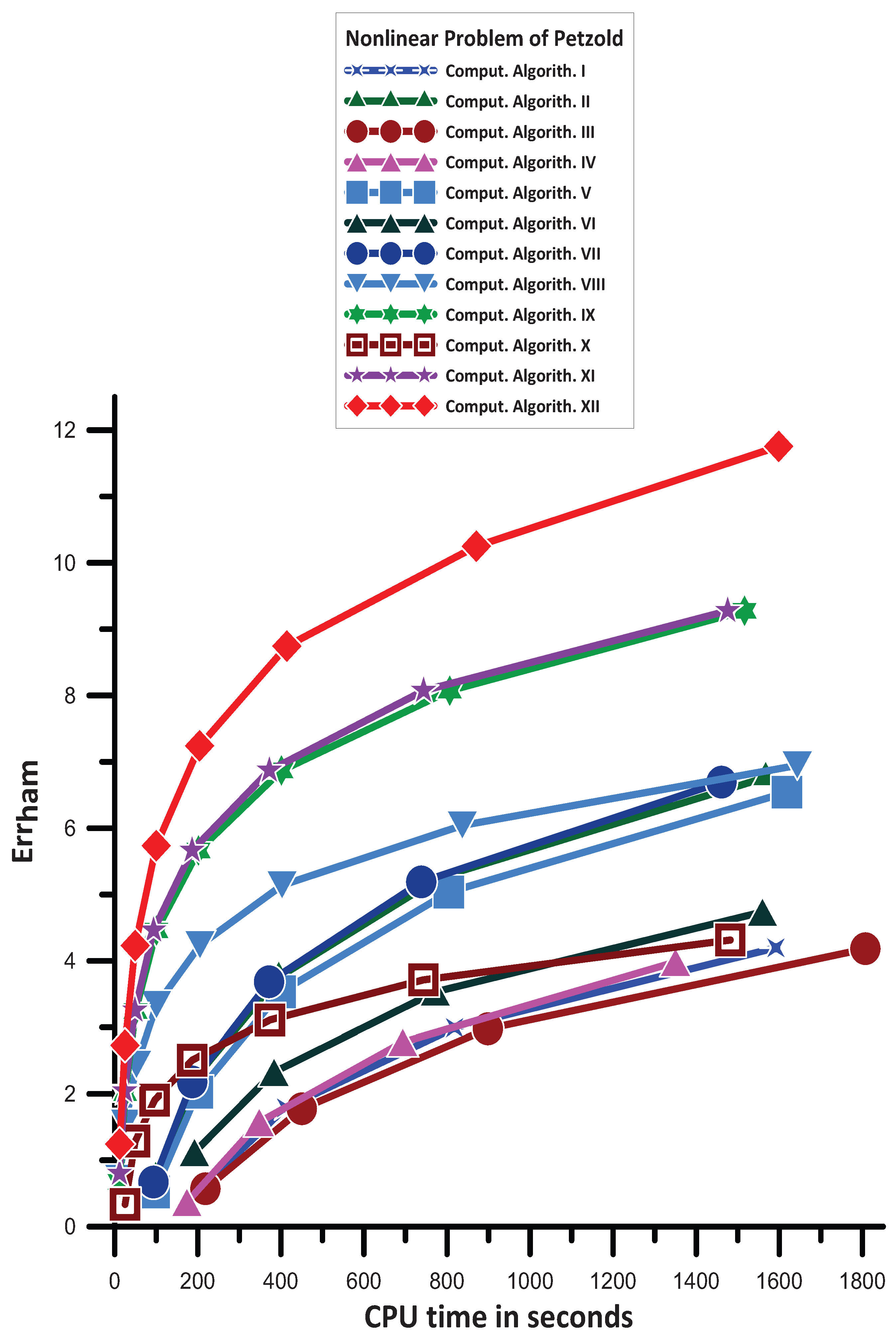
12.3. Nonlinear Problem of Petzold [36]

The following nonlinear problem was examined by Petzold [36] and is taken into account here:

$$\begin{array}{c}\hfill {\mathsf{\Psi }}_1^{\prime }\left(t\right)=\lambda {\mathsf{\Psi }}_2\left(t\right),{\mathsf{\Psi }}_1\left(0\right)=1,\\ \hfill {\mathsf{\Psi }}_2^{\prime }\left(t\right)=-\lambda {\mathsf{\Psi }}_1\left(t\right)+{\displaystyle \frac{\alpha }{\lambda }}sin\left(\lambda x\right),{\mathsf{\Psi }}_2\left(0\right)=-{\displaystyle \frac{\alpha }{2{\lambda }^2}}.\end{array}$$

(96)

The exact solution is

$$\begin{array}{c}\hfill {\mathsf{\Psi }}_1\left(t\right)=\left(1-{\displaystyle \frac{\alpha }{2\lambda }}t\right)cos\left(\lambda t\right),\\ \hfill {\mathsf{\Psi }}_2\left(t\right)=-\left(1-{\displaystyle \frac{\alpha }{2\lambda }}t\right)sin\left(\lambda t\right)-{\displaystyle \frac{\alpha }{2{\lambda }^2}}cos\left(\lambda x\right),\end{array}$$

(97)

where $\lambda =1000$, $\alpha =100$. For this problem, we use $\omega =1000$.

We have discovered the numerical solution to the system of Equation (96) for $0\le t\le 1000$ by using the procedures described in Section 12.1.

Figure 10 provides the data that enable us to see the following:

• Comput. Algorith. I and Comput. Algorith. IV is more efficient than Comput. Algorith. III.
• Comput. Algorith. IV has the same, generally, behavior with Comput. Algorith. I.
• Comput. Algorith. VI is more efficient than Comput. Algorith. IV.
• Comput. Algorith. X gives mixed results. For big step sizes is more efficient than Comput. Algorith. V, Comput. Algorith. VI, and Comput. Algorith. VII. For medium step sizes is more efficient than Comput. Algorith. VI. For very small step sizes is less efficient than Comput. Algorith. VI.
• Comput. Algorith. V gives mixed results. For very big step sizes is less efficient than Comput. Algorith. X. For small step sizes is more efficient than Comput. Algorith. X.
• Comput. Algorith. II has the same, generally, behavior with Comput. Algorith. VII.
• Comput. Algorith. VII is more efficient than Comput. Algorith. V.
• Comput. Algorith. VIII is more efficient than Comput. Algorith. VII.
• Comput. Algorith. IX is more efficient than Comput. Algorith. VIII.
• Comput. Algorith. XI has the same, generally, behavior with Comput. Algorith. IX.
• Finally, Comput. Algorith. XII, is the most efficient one.

12.4. A Nonlinear Orbital Problem [37]

The following nonlinear orbital problem was examined by Simos in [37] and is taken into account here:

$$\begin{array}{ccc}\hfill {\mathsf{\Psi }}_1^{″}\left(t\right)& =& -{\phi }^2{\mathsf{\Psi }}_1\left(t\right)+{\displaystyle \frac{2{\mathsf{\Psi }}_1\left(t\right){\mathsf{\Psi }}_2\left(t\right)-sin\left(2\phi t\right)}{{\left({\mathsf{\Psi }}_1{\left(t\right)}^2+{\mathsf{\Psi }}_2{\left(t\right)}^2\right)}^{\frac{3}{2}}}},{\mathsf{\Psi }}_1\left(0\right)=1,{\mathsf{\Psi }}_1^{\prime }\left(0\right)=0,\hfill \\ \hfill {\mathsf{\Psi }}_2^{″}\left(t\right)& =& -{\phi }^2{\mathsf{\Psi }}_2\left(t\right)+{\displaystyle \frac{{\mathsf{\Psi }}_1{\left(t\right)}^2-{\mathsf{\Psi }}_2{\left(t\right)}^2-cos\left(2\phi t\right)}{{\left({\mathsf{\Psi }}_1{\left(t\right)}^2+{\mathsf{\Psi }}_2{\left(t\right)}^2\right)}^{\frac{3}{2}}}},{\mathsf{\Psi }}_2\left(0\right)=0,{\mathsf{\Psi }}_2^{\prime }\left(0\right)=\phi .\hfill \end{array}$$

(98)

The exact solution is

$${\mathsf{\Psi }}_1\left(t\right)=cos\left(\phi t\right),{\mathsf{\Psi }}_2\left(t\right)=sin\left(\phi t\right).$$

(99)

where $\phi =1000$. For this problem, we use $\omega =1000$.

We have discovered the numerical solution to the system of Equation (99) for $0\le t\le$ 1,000,000 by using the procedures described in Section 12.1.

Figure 11 provides the data that enable us to see the following:

• Comput. Algorith. I, Comput. Algorith. II, Comput. Algorith. III, Comput. Algorith. IV, Comput. Algorith. V, Comput. Algorith. VI, Comput. Algorith. VII, and Comput. Algorith. X are not convergent.
• Comput. Algorith. VIII, Comput. Algorith. IX, Comput. Algorith. XI, and Comput. Algorith. XII have approximately the same behavior and are very efficient.

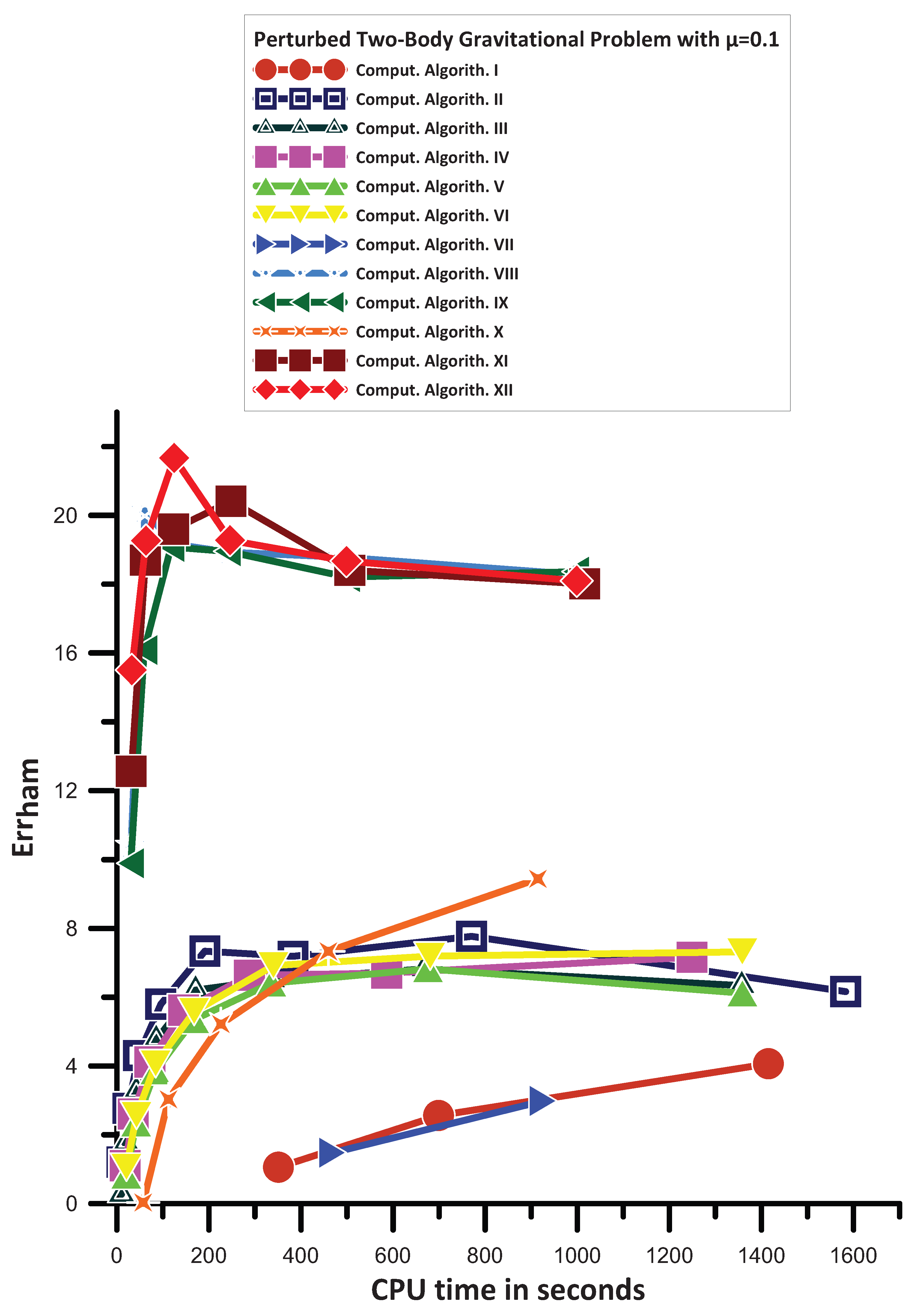
12.5. Perturbed Two–Body Gravitational Problem

We take into account the perturbed two-body Kepler’s problem:

$$\begin{array}{c}\hfill {\mathsf{\Psi }}_1^{″}\left(x\right)=-{\displaystyle \frac{{\mathsf{\Psi }}_1\left(x\right)}{{\left({\mathsf{\Psi }}_1{\left(x\right)}^2+{\mathsf{\Psi }}_2{\left(x\right)}^2\right)}^{\frac{3}{2}}}}-\mu \left(\mu +2\right){\displaystyle \frac{{\mathsf{\Psi }}_1\left(x\right)}{{\left({\mathsf{\Psi }}_1{\left(x\right)}^2+{\mathsf{\Psi }}_2{\left(x\right)}^2\right)}^{\frac{5}{2}}}},\\ \hfill {\mathsf{\Psi }}_1\left(0\right)=1,{\mathsf{\Psi }}_1^{\prime }\left(0\right)=0\\ \hfill {\mathsf{\Psi }}_2^{″}\left(x\right)=-{\displaystyle \frac{{\mathsf{\Psi }}_2\left(x\right)}{{\left({\mathsf{\Psi }}_1{\left(x\right)}^2+{\mathsf{\Psi }}_2{\left(x\right)}^2\right)}^{\frac{3}{2}}}}-\mu \left(\mu +2\right){\displaystyle \frac{{\mathsf{\Psi }}_2\left(x\right)}{{\left({\mathsf{\Psi }}_1{\left(x\right)}^2+{\mathsf{\Psi }}_2{\left(x\right)}^2\right)}^{\frac{5}{2}}}},\\ \hfill {\mathsf{\Psi }}_2\left(0\right)=0,{\mathsf{\Psi }}_2^{\prime }\left(0\right)=1+\mu .\end{array}$$

(100)

The exact solution is

$$\begin{array}{c}\hfill {\mathsf{\Psi }}_1\left(x\right)=cos(x+\mu x),\\ \hfill {\mathsf{\Psi }}_2\left(x\right)=sin(x+\mu x).\end{array}$$

(101)

To solve this problem, we set $\omega ={\displaystyle \frac{\sqrt{1+\mu \left(\mu +2\right)}}{{\left({\mathsf{\Phi }}_1{\left(x\right)}^2+{\mathsf{\Phi }}_2{\left(x\right)}^2\right)}^{\frac{3}{4}}}}$.

Figure 11. Numerical results for the nonlinear orbital problem of [37].

Figure 11. Numerical results for the nonlinear orbital problem of [37].

12.5.1. The Case of $\mu =0.1$

We have discovered the numerical solution to the system of Equation (100) for $0\le t\le$ 100,000 by using the procedures described in Section 12.1.

Figure 12 provides the data that enable us to see the following:

• Comput. Algorith. I has the same, generally, behavior with Comput. Algorith. VII. We note here that Comput. Algorith. I converge to the solution faster than Comput. Algorith. VII
• Comput. Algorith. X gives mixed results. For big step sizes is less efficient than Comput. Algorith. II, Comput. Algorith. II, Comput. Algorith. IV, Comput. Algorith. V, Comput. Algorith. VI, Comput. Algorith. VIII, Comput. Algorith. IX, Comput. Algorith. X, Comput. Algorith. XI, and Comput. Algorith. XII, and is more efficient than Comput. Algorith. I, and Comput. Algorith. VII. For medium step sizes has the same, approximately, accuracy with Comput. Algorith. II, Comput. Algorith. III, Comput. Algorith. IV, Comput. Algorith. V, and Comput. Algorith. VI. For small step sizes is more efficient than all the algorithms except Comput. Algorith. VIII, Comput. Algorith. IX, Comput. Algorith. XI, and Comput. Algorith. XII.
• Comput. Algorith. V is more efficient than Comput. Algorith. I, and Comput. Algorith. VII.
• Comput. Algorith. IV is more efficient than Comput. Algorith. V
• Comput. Algorith. III gives mixed results. For big step sizes is more efficient than Comput. Algorith. V. For small step sizes has the same, generally, behavior with Comput. Algorith. V.
• Comput. Algorith. II is more efficient than Comput. Algorith. III.
• Comput. Algorith. IX gives mixed results. For very big step sizes has the same, generally, behavior with Comput. Algorith. XI. For medium step sizes is less efficient than Comput. Algorith. XI. For small step sizes has the same, generally, behavior with Comput. Algorith. XI.
• Comput. Algorith. VIII has the same, generally, behavior with Comput. Algorith. IX.
• Comput. Algorith. XII for big step sizes is the most efficient one. For medium step sizes is less efficient than Comput. Algorith. XI. For small step sizes has the same, generally, behavior with Comput. Algorith. VIII, Comput. Algorith. IX, Comput. Algorith. XI.

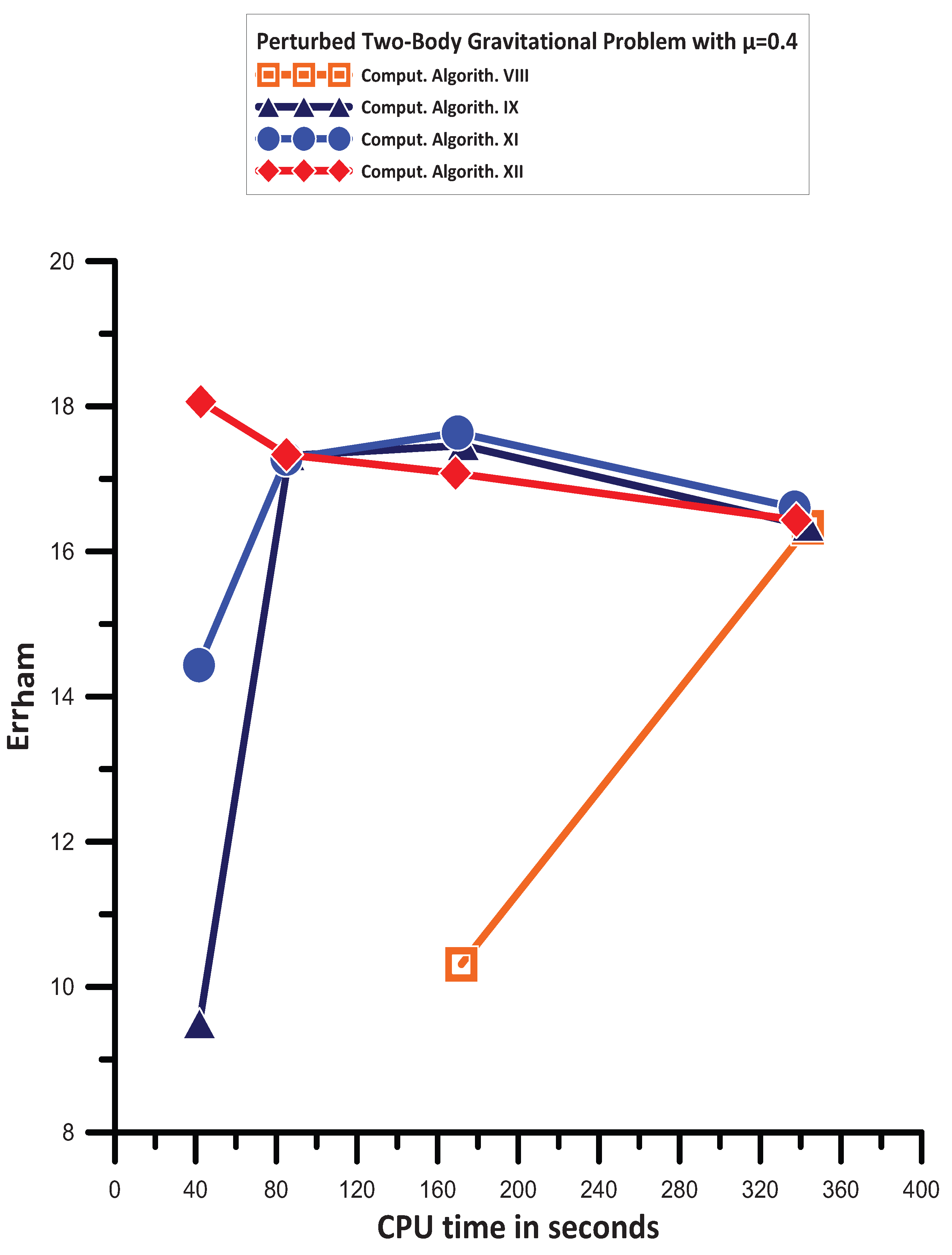
12.5.2. The Case of $\mu =0.4$

We have discovered the numerical solution to the system of Equation (100) for $0\le t\le$ 100,000 by using the procedures described in Section 12.1.

Figure 13 provides the data that enable us to see the following:

• Comput. Algorith. I, Comput. Algorith. II, Comput. Algorith. III, Comput. Algorith. IV, Comput. Algorith. V, Comput. Algorith. VI, Comput. Algorith. VII, and Comput. Algorith. X are not convergent.
• Comput. Algorith. IX is more efficient than Comput. Algorith. VIII.
• Comput. Algorith. XI is more efficient than Comput. Algorith. IX.
• Comput. Algorith. XII for big step sizes is the most efficient one. For medium step sizes is less efficient than Comput. Algorith. IX, and Comput. Algorith. XI. For small step sizes has the same, generally, behavior with Comput. Algorith. VIII, Comput. Algorith. IX, Comput. Algorith. XI.

The best algorithms presented here are based on a careful assessment of all factors:

• The algorithm described in Section 10 has as its primary goals the elimination of the phase–lag and the amplification–factor (phase–fitted and amplification–fitted method) and the vanishing of their first derivatives.
• The algorithm described in Section 9 has as its primary goals the elimination of the phase–lag and the amplification–factor (phase–fitted and amplification–fitted method).
• The algorithm described in Section 7 is centered on the elimination of the phase–lag and amplification–factor (the phase–fitted and amplification–fitted method) and the first derivative of the phase–lag simultaneously.
• The algorithm described in Section 6 is centered on the elimination of the phase–lag and amplification–factor (the phase–fitted and amplification–fitted method) and the first derivative of the amplification–factor simultaneously.

Recently developed frequency-dependent algorithms rely on finding the optimum value of the parameter $\omega$ to assess their effectiveness. This choice is defined explicitly in the issue model for many problems. The parameter $\omega$ may be found using techniques suggested in the literature for cases when this is not easy to accomplish (refer to [38,39]).

Figure 12. Numerical results for perturbed two–body gravitational problem (perturbed Kepler’s problem) with $\mu =0.1$.

Figure 12. Numerical results for perturbed two–body gravitational problem (perturbed Kepler’s problem) with $\mu =0.1$.

Figure 13. Numerical results for perturbed two–body gravitational problem (perturbed Kepler’s problem) with $\mu =0.4$.

Figure 13. Numerical results for perturbed two–body gravitational problem (perturbed Kepler’s problem) with $\mu =0.4$.

12.6. High–Order Ordinary Differential Equations and Partial Differential Equations

Always keep in mind that there are well-established methods for reducing systems of high-order ordinary differential equations to first-order differential equations before attempting to solve them using the newly devised approaches. According to Boyce et al. [33], there are several ways that may be used in this context, such as changing the variables, introducing new variables, rebuilding the system with new variables for each derivative, and so on.

Prior to mentioning the newly introduced techniques, it is worth mentioning that there are already known ways to reduce a system of partial differential equations to a system of first-order differential equations, like the characteristics method (see [40]).

13. Conclusions

Based on the theory and the methodologies for the proofs of the relevant formulae, which we developed in our previous papers [27,28,29], we developed the direct formulae for the computation of the phase–lag and amplification–factor of the Backward Differentiation Formulae (BDF). Using the approach of minimizing or eliminating the phase–lag and amplification–factor to find Backward Differentiation Formulae (BDF) was our main objective in this study. We also looked at how the efficiency of the aforementioned approaches changed when the phase–lag and amplification–factor derivatives were removed. We then detailed several ways to efficiently create methods using the phase–lag and/or amplification–factor and its derivatives, taking into consideration the above. In particular, we developed the following methodologies:

• Methodology for the elimination of the amplification–factor.
• Methodology for the elimination of the amplification–factor and minimization of the phase–lag.
• Methodology for the elimination of the phase–lag and elimination of the amplification–factor.
• Methodology for the elimination of the phase–lag and elimination of the amplification–factor together with elimination of the derivatives of the phase–lag.
• Methodology for the elimination of the phase–lag and elimination of the amplification–factor together with elimination of the derivatives of the amplification–factor.
• Methodology for the elimination of the phase–lag and elimination of the amplification–factor together with the elimination of the derivatives of the phase–Lag and the derivatives of the amplification–Factor

Based on our theoretical and numerical results we conclude that the most efficient methods are the methods in which the coefficients are defined with the requirement of the elimination of the phase–lag and elimination of the amplification–factor, and methods in which the coefficients are defined with the requirement of the elimination of the phase–lag and elimination of the amplification–factor, together with the elimination of the derivatives of the phase–Lag and the derivatives of the amplification–Factor.

Following the aforementioned procedures, a number of Backward Differentiation Formulae (BDF) were developed. We built our methodology on the fourth-order algebraic backward differentiation formula.

The aforementioned approaches were tested on various problems with oscillating solutions to see how well they worked.

All calculations adhered to the IEEE Standard 754 and were executed on a personal computer featuring an x$86-64$ compatible architecture and utilizing a quadruple precision arithmetic data type consisting of 64 bits.

References

- Landau, L.D.; Lifshitz, F.M. Quantum Mechanics; Pergamon: New York, NY, USA, 1965. [Google Scholar]
- Prigogine, I.; Rice, S. (Eds.) Advances in Chemical Physics; New Methods in Computational Quantum Mechanics; John Wiley & Sons: Berlin/Heidelberg, Germany, 1997; Volume 93. [Google Scholar]
- Simos, T.E. Numerical Solution of Ordinary Differential Equations with Periodical Solution. Ph.D. Thesis, National Technical University of Athens, Athens, Greece, 1990. (In Greek). [Google Scholar]
- Ixaru, L.G. Numerical Methods for Differential Equations and Applications; Reidel: Dordrecht, The Netherlands; Boston, MA, USA; Lancaster, UK, 1984. [Google Scholar]
- Quinlan, G.D.; Tremaine, S. Symmetric multistep methods for the numerical integration of planetary orbits. Astron. J. 1990, 100, 1694–1700. [Google Scholar] [CrossRef]
- Lyche, T. Chebyshevian multistep methods for ordinary differential equations. Numer. Math. 1972, 10, 65–75. [Google Scholar] [CrossRef]
- Konguetsof, A.; Simos, T.E. On the construction of Exponentially-Fitted Methods for the Numerical Solution of the Schrödinger Equation. J. Comput. Meth. Sci. Eng. 2001, 1, 143–165. [Google Scholar] [CrossRef]
- Dormand, J.R.; El-Mikkawy, M.E.A.; Prince, P.J. Families of Runge-Kutta-Nyström formulae. IMA J. Numer. Anal. 1987, 7, 235–250. [Google Scholar] [CrossRef]
- Franco, J.M.; Gomez, I. Some procedures for the construction of high-order exponentially fitted Runge-Kutta-Nyström Methods of explicit type. Comput. Phys. Commun. 2013, 184, 1310–1321. [Google Scholar] [CrossRef]
- Franco, J.M.; Gomez, I. Accuracy and linear Stability of RKN Methods for solving second-order stiff problems. Appl. Numer. Math. 2009, 59, 959–975. [Google Scholar] [CrossRef]
- Chien, L.K.; Senu, N.; Ahmadian, A.; Ibrahim, S.N.I. Efficient Frequency-Dependent Coefficients of Explicit Improved Two-Derivative Runge-Kutta Type Methods for Solving Third- Order IVPs. Pertanika J. Sci. Technol. 2023, 31, 843–873. [Google Scholar] [CrossRef]
- Zhai, W.J.; Fu, S.H.; Zhou, T.C.; Xiu, C. Exponentially-fitted and trigonometrically-fitted implicit RKN methods for solving y′′ = f (t, y). J. Appl. Math. Comput. 2022, 68, 1449–1466. [Google Scholar] [CrossRef]
- Fang, Y.L.; Yang, Y.P.; You, X. An explicit trigonometrically fitted Runge-Kutta method for stiff and oscillatory problems with two frequencies. Int. J. Comput. Math. 2020, 97, 85–94. [Google Scholar] [CrossRef]
- Dormand, J.R.; Prince, P.J. A family of embedded Runge-Kutta formulae. J. Comput. Appl. Math. 1980, 6, 19–26. [Google Scholar] [CrossRef]
- Kalogiratou, Z.; Monovasilis, T.; Psihoyios, G.; Simos, T.E. Runge–Kutta type methods with special properties for the numerical integration of ordinary differential equations. Phys. Rep. 2014, 536, 75–146. [Google Scholar] [CrossRef]
- Anastassi, Z.A.; Simos, T.E. Numerical multistep methods for the efficient solution of quantum mechanics and related problems. Phys. Rep. 2009, 482–483, 1–240. [Google Scholar] [CrossRef]
- Chawla, M.M.; Rao, P.S. A Noumerov-Type Method with Minimal Phase-Lag for the Integration of 2nd Order Periodic Initial-Value Problems. J. Comput. Appl. Math. 1984, 11, 277–281. [Google Scholar] [CrossRef]
- Ixaru, L.G.; Rizea, M. A Numerov-like scheme for the numerical solution of the Schrödinger equation in the deep continuum spectrum of energies. Comput. Phys. Commun. 1980, 19, 23–27. [Google Scholar] [CrossRef]
- Raptis, A.D.; Allison, A.C. Exponential-fitting Methods for the numerical solution of the Schrödinger equation. Comput. Phys. Commun. 1978, 14, 1–5. [Google Scholar] [CrossRef]
- Wang, Z.; Zhao, D.; Dai, Y.; Wu, D. An improved trigonometrically fitted P-stable Obrechkoff Method for periodic initial-value problems. Proc. R. Soc. A-Math. Phys. Eng. Sci. 2005, 461, 1639–1658. [Google Scholar] [CrossRef]
- Wang, C.; Wang, Z. A P-stable eighteenth-order six-Step Method for periodic initial value problems. Int. J. Mod. Phys. C 2007, 18, 419–431. [Google Scholar] [CrossRef]
- Shokri, A.; Khalsaraei, M.M. A new family of explicit linear two-step singularly P-stable Obrechkoff methods for the numerical solution of second-order IVPs. Appl. Math. Comput. 2020, 376, 125116. [Google Scholar] [CrossRef]
- Abdulganiy, R.I.; Ramos, H.; Okunuga, S.A.; Majid, Z.A. A trigonometrically fitted intra-step block Falkner method for the direct integration of second-order delay differential equations with oscillatory solutions. Afr. Mat. 2023, 34, 36. [Google Scholar] [CrossRef]
- Lee, K.C.; Senu, N.; Ahmadian, A.; Ibrahim, S.N.I. High-order exponentially fitted and trigonometrically fitted explicit two-derivative Runge-Kutta-type methods for solving third-order oscillatory problems. Math. Sci. 2022, 16, 281–297. [Google Scholar] [CrossRef]
- Fang, Y.L.; Huang, T.; You, X.; Zheng, J.; Wang, B. Two-frequency trigonometrically-fitted and symmetric linear multi-step methods for second-order oscillators. J. Comput. Appl. Math. 2021, 392, 113312. [Google Scholar] [CrossRef]
- Chun, C.; Neta, B. Trigonometrically-Fitted Methods: A Review. Mathematics 2019, 7, 1197. [Google Scholar] [CrossRef]
- Simos, T.E. A New Methodology for the Development of Efficient Multistep Methods for First–Order IVPs with Oscillating Solutions. Mathematics 2024, 12, 504. [Google Scholar] [CrossRef]
- Simos, T.E. Efficient Multistep Algorithms for First–Order IVPs with Oscillating Solutions: II Implicit and Predictor—Corrector Algorithms. Symmetry 2024, 16, 508. [Google Scholar] [CrossRef]
- Simos, T.E. A new methodology for the development of efficient multistep methods for first–order IVPs with oscillating solutions: III The Role of the Derivative of the Phase–Lag and the Derivative of the Amplification–Factor. Axioms 2024, 13, 514. [Google Scholar] [CrossRef]
- Saadat, H.; Kiyadeh, S.H.H.; Karim, R.G.; Safaie, A. Family of phase fitted 3-step second-order BDF methods for solving periodic and orbital quantum chemistry problems. J. Math. Chem. 2024, 62, 1223–1250. [Google Scholar] [CrossRef]
- Stiefel, E.; Bettis, D.G. Stabilization of Cowell’s method. Numer. Math. 1969, 13, 154–175. [Google Scholar] [CrossRef]
- Franco, J.M.; Palacios, M. High-order P-stable multistep methods. J. Comput. Appl. Math. 1990, 30, 1–10. [Google Scholar] [CrossRef]
- Boyce, W.E.; DiPrima, R.C.; Meade, D.B. Elementary Differential Equations and Boundary Value Problems, 11th ed.; John Wiley & Sons: Hoboken, NJ, USA, 2017. [Google Scholar]
- Fehlberg, E. Classical Fifth-, Sixth-, Seventh-, and Eighth-order Runge-Kutta Formulas with Stepsize Control. NASA Technical Report 287. 1968. Available online: https://ntrs.nasa.gov/api/citations/19680027281/downloads/19680027281.pdf (accessed on 15 June 2024).
- Cash, J.R.; Karp, A.H. A variable order Runge–Kutta method for initial value problems with rapidly varying right-hand sides. ACM Trans. Math. Softw. 1990, 16, 201–222. [Google Scholar] [CrossRef]
- Petzold, L.R. An efficient numerical method for highly oscillatory ordinary differential equations. SIAM J. Numer. Anal. 1981, 18, 455–479. [Google Scholar] [CrossRef]
- Simos, T.E. New Open Modified Newton Cotes Type Formulae as Multilayer Symplectic Integrators. Appl. Math. Model. 2013, 37, 1983–1991. [Google Scholar] [CrossRef]
- Ramos, H.; Vigo-Aguiar, J. On the frequency choice in trigonometrically fitted methods. Appl. Math. Lett. 2010, 23, 1378–1381. [Google Scholar] [CrossRef]
- Ixaru, L.G.; Vanden Berghe, G.; De Meyer, H. Frequency evaluation in exponential fitting multistep algorithms for ODEs. J. Comput. Appl. Math. 2002, 140, 423–434. [Google Scholar] [CrossRef]
- Evans, L.C. Partial Differential Equations, 2nd ed.; American Mathematical Society: Providence, RI, USA, 2010; Chapter 3; pp. 91–135. [Google Scholar]
Disclaimer/Publisher’s Note: The statements, opinions and data contained in all publications are solely those of the individual author(s) and contributor(s) and not of MDPI and/or the editor(s). MDPI and/or the editor(s) disclaim responsibility for any injury to people or property resulting from any ideas, methods, instructions or products referred to in the content. |
© 2024 by the author. Licensee MDPI, Basel, Switzerland. This article is an open access article distributed under the terms and conditions of the Creative Commons Attribution (CC BY) license (https://creativecommons.org/licenses/by/4.0/).
Share and Cite
Simos, T.E. A New Methodology for the Development of Efficient Multistep Methods for First–Order IVPs with Oscillating Solutions IV: The Case of the Backward Differentiation Formulae. Axioms 2024, 13, 649. https://doi.org/10.3390/axioms13090649
Simos TE. A New Methodology for the Development of Efficient Multistep Methods for First–Order IVPs with Oscillating Solutions IV: The Case of the Backward Differentiation Formulae. Axioms. 2024; 13(9):649. https://doi.org/10.3390/axioms13090649
Chicago/Turabian StyleSimos, Theodore E. 2024. "A New Methodology for the Development of Efficient Multistep Methods for First–Order IVPs with Oscillating Solutions IV: The Case of the Backward Differentiation Formulae" Axioms 13, no. 9: 649. https://doi.org/10.3390/axioms13090649
APA StyleSimos, T. E. (2024). A New Methodology for the Development of Efficient Multistep Methods for First–Order IVPs with Oscillating Solutions IV: The Case of the Backward Differentiation Formulae. Axioms, 13(9), 649. https://doi.org/10.3390/axioms13090649