Approximation Results: Szász–Kantorovich Operators Enhanced by Frobenius–Euler–Type Polynomials

Abstract

This research focuses on the approximation properties of Kantorovich-type operators using Frobenius–Euler–Simsek polynomials. The test functions and central moments are calculated as part of this study. Additionally, uniform convergence and the rate of approximation are analyzed using the classical Korovkin theorem and the modulus of continuity for Lebesgue measurable and continuous functions. A Voronovskaja-type theorem is also established to approximate functions with first- and second-order continuous derivatives. Numerical and graphical analyses are presented to support these findings. Furthermore, a bivariate sequence of these operators is introduced to approximate a bivariate class of Lebesgue measurable and continuous functions in two variables. Finally, numerical and graphical representations of the error are provided to check the rapidity of convergence.

1. Introduction and Preliminaries

Bernstein (1913) [1] introduced a sequence of polynomials to present the simplest proof for an elegant theorem on the basis of Weierstrass (1885) [2], which is termed the Weierstrass approximation theorem in terms of a binomial probability distribution as follows:

$$\begin{array}{c}\hfill {\mathbf{B}}_n(f;y)={\displaystyle \sum _{k=0}^n}{}_{n,k}\left(y\right)f\left({\displaystyle \frac{k}{n}}\right),\mathrm{n}\in \mathbb{N},\end{array}$$

(1)

where ${}_{n,k}\left(y\right)=\left({\displaystyle \genfrac{}{}{0pt}{}{n}{k}}\right)y^k{(1-y)}^{n-k}$ and $y\in [0,1]$. He found that ${\mathbf{B}}_n(f;.)\rightrightarrows f$ for every bounded function f defined on $[0,1]$, where ⇉ depicts the convergence, is uniform.

Kantorovich [3] extended (1) to approximating Lebesgue measurable functions. For $n\in \mathbb{N}$ and $f\in L^p[0,1]$ where $1\le p<\infty$, the Kantorovich operators $K_n:L^p\left([0,1]\right)\to L^p\left([0,1]\right)$ are defined as

$$K_n(f;y)=(n+1)\sum _{k=0}^n{}_{n,k}\left(y\right){\int }_{{\displaystyle \frac{k}{n+1}}}^{{\displaystyle \frac{k+1}{n+1}}}f\left(t\right)dt,$$

(2)

where ${}_{n,k}\left(y\right)=\left({\displaystyle \genfrac{}{}{0pt}{}{n}{k}}\right)y^k{(1-y)}^{n-k}$ and the Kantorovich operators converge almost everywhere with a function on $[0,1]$. Nowadays, operator theory connects various disciplines of science like engineering and medical sciences such as robotics, CAGD, HIV research, etc. [4,5,6,7,8,9]. In the past decade, many mathematicians have constructed various modifications of the operators defined by (1) to achieve better flexibility in the approximation properties over bounded and unbounded intervals in various functional spaces, e.g., $\ddot{\mathrm{O}}$zger et al. [10,11], Cai et al. [12,13], Aslan [14,15], Acu et al. [16,17,18], Mohiuddine et al. [19,20], Mursaleen et al. [21,22], Bustamante [23], Ozsarac et al. [24], Khan et al. [25], Nasiruzzaman [26], Braha et al. [27], Rao et al. [28,29], and Çetin et al. [30,31]. In view of polynomial classes, which are an active field of research as a special function field, we recall a class of polynomials by Simsek [32] which are termed Frobenius–Euler–Simsek-type numbers and polynomials ${\left\{l_k(y;v)\right\}}_{k=0}^{\infty }$ associated with the generating function as

$$F_l(y;w,v):={\displaystyle \frac{w^v}{{\displaystyle \prod _{j=0}^{v-1}}(e^w-j)}}{e}^{wy}=\sum _{k=0}^{\infty }{l}_k(y;v){\displaystyle \frac{w^k}{k!}}.$$

(3)

For $y=0$, we yield Frobenius–Euler–Simsek-type numbers as

$$F_l(0;w,v):={\displaystyle \frac{w^v}{{\displaystyle \prod _{j=0}^{v-1}}(e^w-j)}}=\sum _{k=0}^{\infty }{l}_k(0;v){\displaystyle \frac{w^k}{k!}}.$$

Putting $v=2$ into the above equation, we acquire

$$F_l(y;w,2):={\displaystyle \frac{w^2}{e^w(e^w-1)}}{e}^{wy}=\sum _{k=0}^{\infty }{l}_k(y;2){\displaystyle \frac{w^k}{k!}}.$$

(4)

For detailed information and applications, see [33,34]. Motivated by the above development in the literature, we introduce a new connection to Kantorovich-type operators involving Frobenius–Euler–Simsek-type numbers as follows:

$$K_n(f;y)={\displaystyle \frac{n}{c_n}}(e^2-e)e^{-{\displaystyle \frac{n}{c_n}}y}\sum _{k=0}^{\infty }{\displaystyle \frac{l_k\left(\frac{n}{c_n}y;2\right)}{k!}}{\int }_{{\displaystyle \frac{k}{n}}{c}_n}^{{\displaystyle \frac{(k+1)}{n}}{c}_n}f\left(t\right)dt,f\in L^p[0,\infty ),$$

(5)

where $1\le p<\infty$ and ${\left\{c_n\right\}}_1^{\infty }$ is a positive increasing sequence of real numbers such that $\underset{n\to \infty }{lim}{c}_n=\infty$ and $\underset{n\to \infty }{lim}{\displaystyle \frac{c_n}{n}}=0$. Now, we discuss some preliminary results to investigate the approximation properties of $K_n(.;.)$ in (5) as follows:

Lemma 1

([35]). In view of (4), one has

$$\begin{array}{ccc}\hfill {\displaystyle \frac{d}{dw}}{F}_l(y;w,2)& =& {\displaystyle \frac{w{e}^{w(y-1)}(-yw+e^w(wy-2w+2)+w-2)}{{(e^w-1)}^2}};\hfill \\ \hfill {\displaystyle \frac{d^2}{d{w}^2}}{F}_l(y;w,2)& =& {\displaystyle \frac{e^{w(y-1)}}{{(e^w-1)}^3}}[w^2{(y-1)}^2+w{e}^2(w^2{(y-2)}^2+4w(y-2)+2)\hfill \\ & +& 4w(y-1)+2-e^w(w^2(2y^2-6y+3)+4w(2y-3)+4)].\hfill \end{array}$$

Lemma 2.

In light of the generating function introduced in (4), we yield

$$\begin{array}{cc}\hfill {\displaystyle \sum _{k=0}^{\infty }}{\displaystyle \frac{l_k\left(\frac{n}{c_n}y;2\right)}{k!}}& ={\displaystyle \frac{e^{\frac{n}{c_n}y}}{e^2-e}},\hfill \\ \hfill {\displaystyle \sum _{k=0}^{\infty }}k{\displaystyle \frac{l_k\left(\frac{n}{c_n}y;2\right)}{k!}}& ={\displaystyle \frac{ny{e}^{\frac{n}{c_n}y}}{c_n(e^2-e)}}-{\displaystyle \frac{e^{\frac{n}{c_n}y}}{e{(e-1)}^2}},\hfill \\ \hfill {\displaystyle \sum _{k=0}^{\infty }}{k}^2{\displaystyle \frac{l_k\left(\frac{n}{c_n}y;2\right)}{k!}}& ={\left({\displaystyle \frac{n}{c_n}}\right)}^2{\displaystyle \frac{e^{\frac{n}{c_n}y}{y}^2}{e(e-1)}}-{\displaystyle \frac{2n}{c_n}}{\displaystyle \frac{e^{\frac{n}{c_n}y}y}{(e-1)}}-{\displaystyle \frac{2e^2-5e+1}{e{(e-1)}^3}}{e}^{{\displaystyle \frac{n}{c_n}}y}.\hfill \end{array}$$

Proof. 

On account of Lemma 1, we can prove Lemma 2 considering $w=1$ and y as ${\displaystyle \frac{n}{c_n}}y$. □

Lemma 3.

Let $f_i\left(t\right)=t^i$, $i\in \{0,1,2\}$. Then, we obtain

$$\begin{array}{cc}\hfill K_n(f_0;y)& =1,\hfill \\ \hfill K_n(f_1,y)& =y-{\displaystyle \frac{c_n}{n}}{\displaystyle \frac{1}{(e-1)}}+{\displaystyle \frac{c_n}{2n}},\hfill \\ \hfill K_n(f_2,y)& =y^2+{\displaystyle \frac{c_n}{n}}(1-2e)y+{\left({\displaystyle \frac{c_n}{n}}\right)}^2\left[{\displaystyle \frac{13-2e-5e^2}{3{(e-1)}^2}}\right].\hfill \end{array}$$

Proof. 

On account of proving Lemma 3 and from the operators $K_n(.;.)$ in (5), we have

$$\begin{array}{c}\hfill K_n(f_i;y)={\displaystyle \frac{n}{c_n}}(e^2-e)e^{-{\displaystyle \frac{n}{c_n}}y}{\displaystyle \sum _{k=0}^{\infty }}{\displaystyle \frac{l_k\left(\frac{n}{c_n}y;2\right)}{k!}}{\int }_{{\displaystyle \frac{k}{n}}{c}_n}^{{\displaystyle \frac{(k+1)}{n}}{c}_n}{t}^{i}dt.\end{array}$$

For $i=0$,

$$\begin{array}{ccc}\hfill K_n(f_0;y)& =& {\displaystyle \frac{n}{c_n}}(e^2-e)e^{-{\displaystyle \frac{n}{c_n}}y}{\displaystyle \sum _{k=0}^{\infty }}{\displaystyle \frac{l_k\left(\frac{n}{c_n}y;2\right)}{k!}}{\int }_{{\displaystyle \frac{k}{n}}{c}_n}^{{\displaystyle \frac{(k+1)}{n}}{c}_n}1dt\hfill \\ & =& {\displaystyle \frac{n}{c_n}}(e^2-e)e^{-{\displaystyle \frac{n}{c_n}}y}{\displaystyle \sum _{k=0}^{\infty }}{\displaystyle \frac{l_k\left(\frac{n}{c_n}y;2\right)}{k!}}\left[{\displaystyle \frac{(k+1)}{n}}{c}_n-{\displaystyle \frac{k}{n}}{c}_n\right]\hfill \\ & =& (e^2-e)e^{-{\displaystyle \frac{n}{c_n}}y}{\displaystyle \sum _{k=0}^{\infty }}{\displaystyle \frac{l_k\left(\frac{n}{c_n}y;2\right)}{k!}}=1.\hfill \end{array}$$

For $i=1$, we yield

$$\begin{array}{ccc}\hfill K_n(f_1;y)& =& {\displaystyle \frac{n}{c_n}}(e^2-e)e^{-{\displaystyle \frac{n}{c_n}}y}{\displaystyle \sum _{k=0}^{\infty }}{\displaystyle \frac{l_k\left(\frac{n}{c_n}y;2\right)}{k!}}{\int }_{{\displaystyle \frac{k}{n}}{c}_n}^{{\displaystyle \frac{(k+1)}{n}}{c}_n}tdt\hfill \\ & =& {\displaystyle \frac{n}{c_n}}(e^2-e)e^{-{\displaystyle \frac{n}{c_n}}y}{\displaystyle \sum _{k=0}^{\infty }}{\displaystyle \frac{l_k\left(\frac{n}{c_n}y;2\right)}{k!}}{\left[{\displaystyle \frac{t^2}{2}}\right]}_{{\displaystyle \frac{k}{n}}{c}_n}^{{\displaystyle \frac{k+1}{n}}{c}_n}\hfill \\ & =& {\displaystyle \frac{n}{c_n}}(e^2-e)e^{-{\displaystyle \frac{n}{c_n}}y}{\displaystyle \sum _{k=0}^{\infty }}{\displaystyle \frac{l_k\left(\frac{n}{c_n}y;2\right)}{k!}}{\displaystyle \frac{1}{2}}\left[{\left({\displaystyle \frac{k+1}{n}}\right)}^2{c}_n^2-{\displaystyle \frac{k^2}{n^2}}{c}_n^2\right]\hfill \\ & =& {\displaystyle \frac{c_n}{n}}(e^2-e)e^{-{\displaystyle \frac{n}{c_n}}y}{\displaystyle \sum _{k=0}^{\infty }}k{\displaystyle \frac{l_k\left(\frac{n}{c_n}y;2\right)}{k!}}\hfill \\ & +& {\displaystyle \frac{c_n}{2n}}(e^2-e)e^{-{\displaystyle \frac{n}{c_n}}y}{\displaystyle \sum _{k=0}^{\infty }}{\displaystyle \frac{l_k\left(\frac{n}{c_n}y;2\right)}{k!}}.\hfill \end{array}$$

In light of Lemma 2, we obtain

$$\begin{array}{ccc}\hfill K_n(f_1;y)& =& y+{\displaystyle \frac{c_n}{n}}\left({\displaystyle \frac{1}{2}}-{\displaystyle \frac{1}{e-1}}\right).\hfill \end{array}$$

For $i=2$,

$$\begin{array}{ccc}\hfill K_n(f_2;y)& =& {\displaystyle \frac{n}{c_n}}(e^2-e)e^{-{\displaystyle \frac{n}{c_n}}y}{\displaystyle \sum _{k=0}^{\infty }}{\displaystyle \frac{l_k\left(\frac{n}{c_n}y;2\right)}{k!}}{\int }_{{\displaystyle \frac{k}{n}}{c}_n}^{{\displaystyle \frac{(k+1)}{n}}{c}_n}{t}^{2}dt\hfill \\ & =& {\displaystyle \frac{n}{c_n}}(e^2-e)e^{-{\displaystyle \frac{n}{c_n}}y}{\displaystyle \sum _{k=0}^{\infty }}{\displaystyle \frac{l_k\left(\frac{n}{c_n}y;2\right)}{k!}}{\left[{\displaystyle \frac{t^3}{3}}\right]}_{{\displaystyle \frac{k}{n}}{c}_n}^{{\displaystyle \frac{k+1}{n}}{c}_n}\hfill \\ & =& {\displaystyle \frac{n}{c_n}}(e^2-e)e^{-{\displaystyle \frac{n}{c_n}}y}{\displaystyle \sum _{k=0}^{\infty }}{\displaystyle \frac{l_k\left(\frac{n}{c_n}y;2\right)}{k!}}{\displaystyle \frac{1}{3}}\left[{\left({\displaystyle \frac{k+1}{n}}\right)}^3{c}_n^3-{\displaystyle \frac{k^3}{n^3}}{c}_n^3\right].\hfill \end{array}$$

Similarly, in light of Lemma 2, we find

$$\begin{array}{cc}\hfill K_n(f_2;y)& =y^2+{\displaystyle \frac{c_n}{n}}(1-2e)y+{\left({\displaystyle \frac{c_n}{n}}\right)}^2\left[{\displaystyle \frac{13-2e-5e^2}{3{(e-1)}^2}}\right].\end{array}$$

□

Remark 1.

The sequence of operators introduced in (5) is linear, i.e., for all $k_1,k_2\in \mathbb{R}$ and $f,g\in L^p[0,\infty )$, we yield

$$\begin{array}{c}\hfill K_n(k_{1}f+k_{2}g;y)=k_1{K}_n(f;y)+k_2{K}_n(g;y).\end{array}$$

Remark 2.

The sequence of operators introduced in (5) is positive, i.e., $K_n(f;y)\ge 0$ for $f\ge 0$.

Lemma 4.

For the sequence of operators given in (5) and $f_i^y\left(t\right)={(t-y)}^i,i\in \{0,1,2\}$, the following equalities hold:

$$\begin{array}{ccc}\hfill K_n(f_o^y;y)& =& 1,\hfill \\ \hfill K_n(f_1^y;y)& =& {\displaystyle \frac{c_n}{n}}\left({\displaystyle \frac{1}{2}}-{\displaystyle \frac{1}{e-1}}\right),\hfill \\ \hfill K_n(f_2^y;y)& =& {\displaystyle \frac{c_n}{n}}{\displaystyle \frac{2(1+e-e^2)}{e-1}}y+{\left({\displaystyle \frac{c_n}{n}}\right)}^2\left({\displaystyle \frac{13-2e-5e^2}{3{(e-1)}^2}}\right).\hfill \end{array}$$

Proof. 

Using (5) and the linearity property, we obtain

$$\begin{array}{ccc}\hfill K_n(f_o^y;y)& =& K_n(f_0;y)=1,\hfill \\ \hfill K_n(f_1^y;y)& =& K_n(t-y;y)=K_n(f_1;y)-y{K}_n(f_0;y),\hfill \\ \hfill K_n(f_2^y;y)& =& K_n({(t-y)}^2;y)=K_n(f_2;y)-2y{K}_n(f_1;y)+y^2{K}_n(f_0;y).\hfill \end{array}$$

In light of Lemma 3, we arrive at the desired result. □

This manuscript presents the approximation results for the operators defined by (5). It covers several key aspects: the uniform convergence and the pointwise and Voronovskaja-type theorems which deal with functions that grow at different rates. It also extends the operators to a bivariate case, analyzing their uniform rate of approximation and approximation order. Finally, it examines how these operators perform in different functional spaces to demonstrate their improved approximation behavior.

2. Approximation Properties—Uniform Convergence and the Approximation Order

Definition 1

([36]). Let $f\in C_B[0,\infty )$ (the space of a bounded and continuous function). Then, the modulus of continuity is introduced as

$$\begin{array}{c}\hfill \omega (f;\tilde{\delta })={\displaystyle \underset{|y_1-y_2|\le \tilde{\delta }}{sup}}|f\left(y_1\right)-f\left(y_2\right)|,y_1,y_2\in [0,\infty ),\end{array}$$

(6)

and

$$\begin{array}{c}\hfill |f\left(y_1\right)-f\left(y_2\right)|\le \left(1+{\displaystyle \frac{|y_1-y_2|}{\tilde{\delta }}}\right)\omega (f;\tilde{\delta }).\end{array}$$

(7)

Theorem 1.

Let $K_n(.;.)$ be given in (5) and for all $f\in L^p[0,\infty )$. Then, $K_n(f;.)$ uniformly converges to f on a closed and bounded subset of $[0,\infty ).$

Proof. 

Based on the classical Korovkin theorem [37], it is enough to show that

$$\begin{array}{c}\hfill K_n(f_i;y)=y^i,i\in \{0,1,2\},\end{array}$$

uniformly on every closed and bounded subset of $[0,\infty )$. Operating Lemma 3, we quickly reach the required result. □

The next result is the study of the order of approximation of (5) in terms of the modulus of continuity in Equation (6) as

Theorem 2.

For $f\in C_B[0,\infty )$ and the sequence of operators $K_n(.;.)$ in Equation (5), we have

$$\begin{array}{c}\hfill |K_n(f;y)-f\left(y\right)|\le 2\omega (f;\tilde{\delta }),\end{array}$$

where $\tilde{\delta }=\sqrt{K_n(f_2^y;y)}$.

Proof. 

With the definition of Equation (5), we yield

$$\begin{array}{ccc}\hfill \left|K_n(f;y)-f\left(y\right)\right|& =& K_n\left(\left|f\right(t)-f(y\left)\right|;y\right).\hfill \end{array}$$

In view of Equation (7), we have

$$\begin{array}{c}\hfill \left|K_n(f;y)-f\left(y\right)\right|\le K_n\left(\left(1+{\displaystyle \frac{|t-y|}{\tilde{\delta }}}\right)\omega (f;\tilde{\delta });y\right)\\ \hfill =\left\{1+{\displaystyle \frac{1}{\tilde{\delta }}}{K}_n\left(\right|t-y\left|\right)\right\}\omega (f;\tilde{\delta }).\end{array}$$

Using the Cauchy–Schwarz inequality, we yield

$$\begin{array}{ccc}\hfill |K_n(f;y)-f\left(y\right)|& \le & \left\{1+{\displaystyle \frac{1}{\tilde{\delta }}}\sqrt{\left(K_n{(t-y)}^2;y\right)}\right\}\omega (f;\tilde{\delta })\hfill \\ & \le & \left\{1+{\displaystyle \frac{\sqrt{K_n(f_2^y;y)}}{\tilde{\delta }}}\right\}\omega (f;\tilde{\delta }).\hfill \end{array}$$

On choosing $\tilde{\delta }=\sqrt{K_n(f_2^y;y)}$, we yield

$$\begin{array}{c}\hfill |K_n(f;y)-f\left(y\right)|\le 2\omega (f;\tilde{\delta }).\end{array}$$

Thus, we prove the required result. □

Now, we introduce the Voronovskaja-type theorem to approximate functions with continuous first- and second-order derivatives, using the operators from (5), as follows:

Theorem 3.

Let $f,f^{\prime },f^{″}\in C^2[0,\infty )\bigcap E=\{f:{\displaystyle \frac{f\left(y\right)}{1+y^2}}$ converge as $y\to \infty \}$ and $y\in [0,\infty ).$ Then, we receive

$$\begin{array}{ccc}\hfill {\displaystyle \underset{n\to \infty }{lim}}{\displaystyle \frac{n}{c_n}}(K_n(f;y)-f\left(y\right))& =& f^{\prime }\left(y\right)\left({\displaystyle \frac{1}{2}}-{\displaystyle \frac{1}{e-1}}\right)+{\displaystyle \frac{f^{″}\left(y\right)}{2!}}\left({\displaystyle \frac{2(1+e-e^2)}{e-1}}\right)y.\hfill \end{array}$$

Proof. 

To approximate the functions, we first recall the Taylor series expansion:

$$\begin{array}{c}\hfill f\left(t\right)=f\left(y\right)+f^{\prime }\left(y\right)(t-y)+f^{″}\left(y\right){\displaystyle \frac{{(t-y)}^2}{2!}}+\xi (t,y){(t-y)}^2,\end{array}$$

(8)

where $\xi (t,y)$ is the Peano remainder such that $\xi (t,y)\in C[0,\infty )\cap E$ and ${lim}_{t\to y}\xi (t,y)=0$. Applying the operators $K_n(.;.)$ defined in Equation (5) to Equation (8), we have

$$\begin{array}{c}\hfill K_n(f;y)=f\left(y\right)+f^{\prime }\left(y\right)K_n(f_1^y;y)+{\displaystyle \frac{f^{″}}{2!}}{K}_n(f_2^y;y)+K_n(\xi (t,y){(t-y)}^2;y).\end{array}$$

(9)

By applying the limit to both sides of the expression in (9), we obtain

$$\begin{array}{ccc}\hfill {\displaystyle \underset{n\to \infty }{lim}}{\displaystyle \frac{n}{c_n}}(K_n(f;y)-f\left(y\right))& =& f^{\prime }\left(y\right){\displaystyle \underset{n\to \infty }{lim}}{\displaystyle \frac{n}{c_n}}{K}_n(f_1^y;y)+{\displaystyle \frac{f^{″}}{2!}}{\displaystyle \underset{n\to \infty }{lim}}{\displaystyle \frac{n}{c_n}}{K}_n(f_2^y;y)\hfill \\ \hfill & +& {\displaystyle \underset{n\to \infty }{lim}}{\displaystyle \frac{n}{c_n}}{K}_n(\xi (t,y){(t-y)}^2;y)\hfill \\ \hfill & =& f^{\prime }\left(y\right)\left({\displaystyle \frac{1}{2}}-{\displaystyle \frac{1}{e-1}}\right)+{\displaystyle \frac{f^{″}\left(y\right)}{2!}}\left({\displaystyle \frac{2(1+e-e^2)}{e-1}}\right)y\hfill \\ & +& {\displaystyle \underset{n\to \infty }{lim}}{\displaystyle \frac{n}{c_n}}{K}_n(\xi (t,y){(t-y)}^2;y).\hfill \end{array}$$

(10)

The last term of the equation is obtained using the Cauchy–Schwarz inequality:

$$\begin{array}{c}\hfill {\displaystyle \frac{n}{c_n}}{K}_n(\xi (t,y){(t-y)}^2;y)\le \sqrt{{\left({\displaystyle \frac{n}{c_n}}\right)}^2{K}_n({(t-y)}^4;y)K_n({\xi }^2(t,y);y)}.\end{array}$$

(11)

From Equations (10) and (11), Lemma 4, and ${lim}_{n\to \infty }{K}_n({\xi }^2(t,y);y)=0$, we yield

$$\begin{array}{ccc}\hfill {\displaystyle \underset{c_n\to \infty }{lim}}{\displaystyle \frac{n}{c_n}}(K_n(f;y)-f\left(y\right))& =& f^{\prime }\left(y\right)\left({\displaystyle \frac{1}{2}}-{\displaystyle \frac{1}{e-1}}\right)\hfill \\ & +& {\displaystyle \frac{f^{″}\left(y\right)}{2!}}\left({\displaystyle \frac{2(1+e-e^2)}{e-1}}\right)y.\hfill \end{array}$$

which proves the required result. □

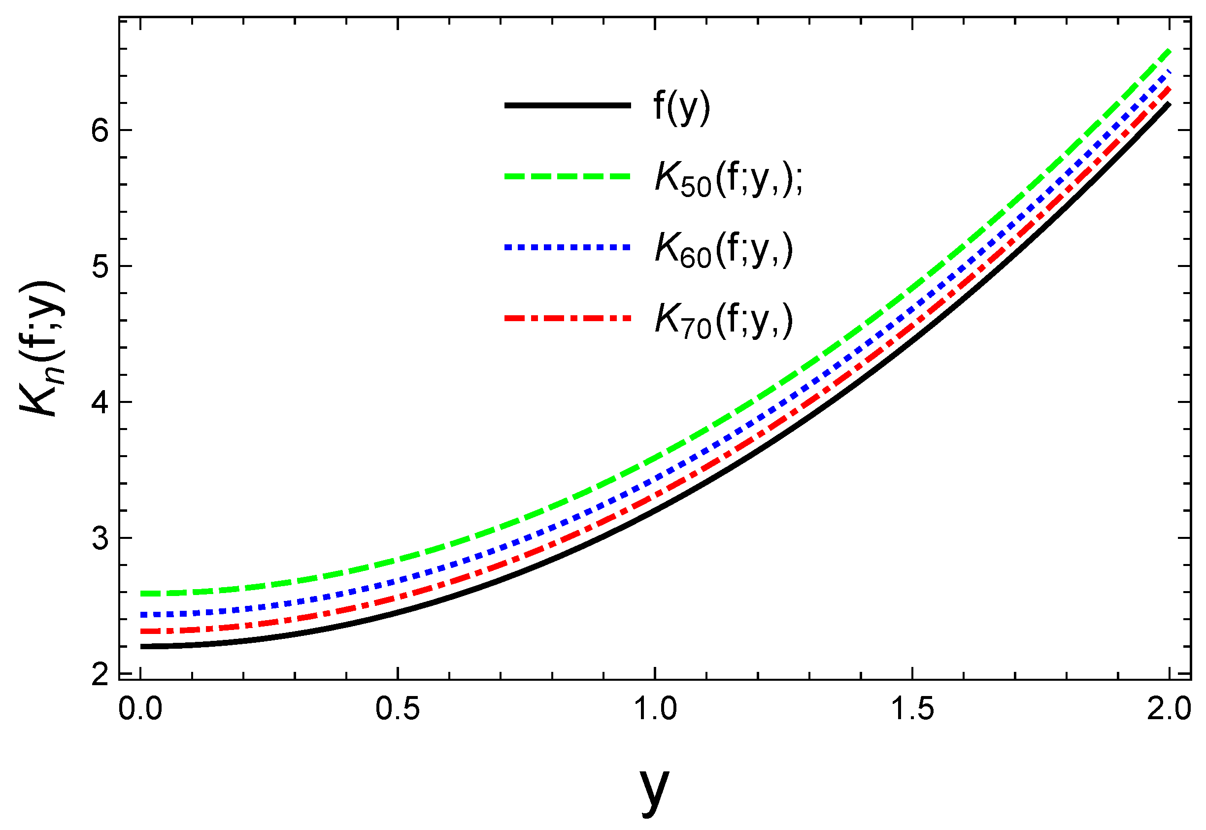
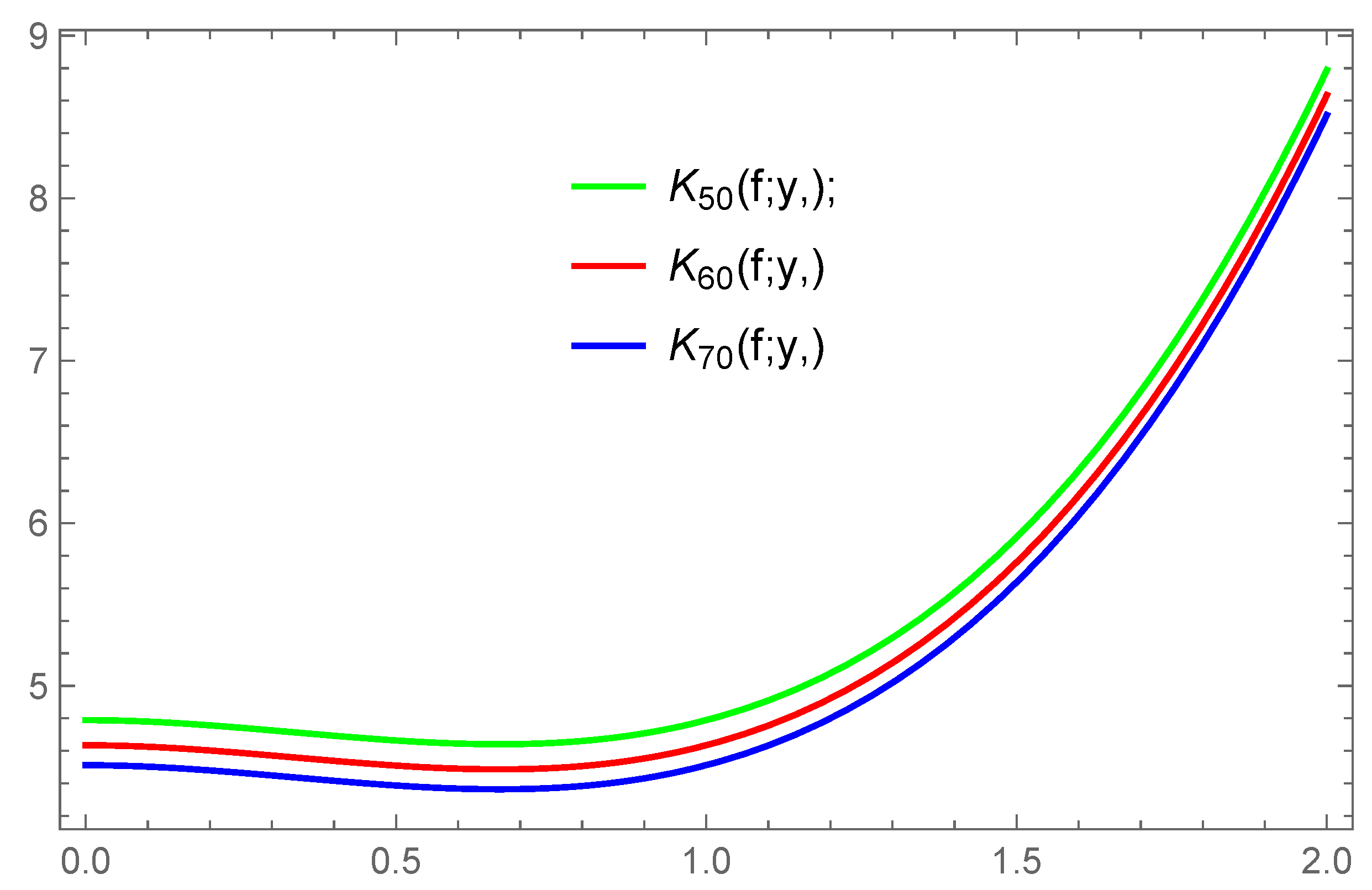
3. Graphical and Numerical Approaches to a Convergence Analysis

In this section, we analyze the convergence properties of the operators defined in (5) for different values of n, specifically $n=50$, $n=60$, and $n=70$. Figure 1 visualizes the convergence behavior, demonstrating the impact of increasing n on the operator’s performance, while Figure 2 illustrates the approximation error trends. The numerical errors, computed using the formula $E_n(f;y)=\left|K_n(f;y)-f\left(y\right)\right|$ for the function $f\left(y\right)=y^2+2$, are presented in

Table 1. The error approximation of the operators $K_n(f;y)$ to $f\left(y\right)$.

y	$|{\mathit{K}}_{50}(\mathit{f};\mathit{y})-\mathit{f}\left(\mathit{y}\right)|$	$|{\mathit{K}}_{60}(\mathit{f};\mathit{y})-\mathit{f}\left(\mathit{y}\right)\left|\right)$	$|{\mathit{K}}_{70}(\mathit{f};\mathit{y})-\mathit{f}\left(\mathit{y}\right)|$
0.2	4.82078	4.66625	4.54366
0.4	4.88478	4.73025	4.60766
0.6	4.93278	4.77825	4.65566
0.8	4.91678	4.77825	4.63966
1.0	4.86978	4.76228	4.59266
1.2	4.78878	4.71525	4.51166
1.4	4.50078	4.63425	4.22366
1.6	4.00478	4.34625	3.72766
1.8	3.25278	3.85025	2.97566
2.0	2.19678	3.09825	1.91966

. These errors provide a quantitative measure of the approximation accuracy for different values of n and highlight the rate of convergence as n increases. From Figure 1, we observe that larger values of n improve the operators’ convergence to $f\left(y\right)$, while Figure 2 shows a consistent reduction in the approximation error, demonstrating the effectiveness of the operators for higher values of n. Table 1 further confirms that the error decreases significantly as n increases, validating the theoretical convergence properties. This numerical analysis not only supports the theoretical findings but also offers a practical understanding of the operator’s behavior. By evaluating the errors across different y values, we gain insights into the robustness and efficiency of the operators in approximating $f\left(y\right)$, which is essential for applications requiring high accuracy.

4. Local Approximation Results

Now, we recall a Lipschitz-type space [38], which is defined as

$$\begin{array}{c}\hfill Li{p}_{\tilde{M}}^{{\phi }_1,{\phi }_2}\left(\tau \right):=\{f\in {\tilde{C}}_{\tilde{B}}[0,\infty ):|f\left(t\right)-f\left(y\right)|\le \tilde{M}{\displaystyle \frac{{|t-y|}^{\tau }}{{(t+{\phi }_{1}y+{\phi }_2{y}^2)}^{\frac{\tau }{2}}}}:y,t\in (0,\infty )\},\end{array}$$

where $\tilde{M}>0$, $0<\tau \le 1$ and ${\phi }_1,{\phi }_2>0$.

Theorem 4.

Let $K_n(.;.)$ be the operator given by (4). Then, for $f\in Li{p}_M^{{\phi }_1,{\phi }_2}\left(\tau \right)$, we have

$$\begin{array}{c}\hfill |K_n(f;y)-f\left(y\right)|\le \tilde{M}{\left({\displaystyle \frac{\lambda \left(y\right)}{{\phi }_{1}y+{\phi }_2{y}^2}}\right)}^{{\displaystyle \frac{\tau }{2}}},\end{array}$$

(12)

where $0<\tau \le 1$, ${\phi }_1,{\phi }_2\in (0,\infty )$ and $\lambda \left(y\right)=K_n(f_2^y;y)$.

Proof. 

For $\tau =1$ and $y>0$, we yield

$$\begin{array}{cc}\hfill |K_n(f;y)-f\left(y\right)|& \le K_n\left(\right|f\left(t\right)-f\left(y\right)|;y)\hfill \\ \hfill & \le \tilde{M}{K}_n\left({\displaystyle \frac{|t-y|}{{(t+{\phi }_{1}y+{\phi }_2{y}^2)}^{\frac{1}{2}}}};y\right).\hfill \end{array}$$

Since ${\displaystyle \frac{1}{t+{\phi }_{1}y+{\phi }_2{y}^2}<\frac{1}{{\phi }_{1}y+{\phi }_2{y}^2}}$, for all $y\in (0,\infty )$, we yield

$$\begin{array}{cc}\hfill |K_n(f;y)-f\left(y\right)|& \le {\displaystyle \frac{\tilde{M}}{{({\phi }_{1}y+{\phi }_2{y}^2)}^{\frac{1}{2}}}}{\left(K_n(f_2;y)\right)}^{{\displaystyle \frac{1}{2}}}\hfill \\ \hfill & \le \tilde{M}{\left({\displaystyle \frac{\lambda \left(y\right)}{{\phi }_{1}y+{\phi }_2{y}^2}}\right)}^{{\displaystyle \frac{1}{2}}}.\hfill \end{array}$$

This implies that Theorem 4 holds for $\tau =1$. Next, we consider a case where $\tau \in (0,1)$, and in view of Hölder’s inequality using $p={\displaystyle \frac{2}{\tau }}$ and $q={\displaystyle \frac{2}{2-\tau }}$, obtain

$$\begin{array}{cc}\hfill |K_n(f;y)-f\left(y\right)|& \le {(K_n{\left(\right|f\left(t\right)-f\left(y\right)|}^{{\displaystyle \frac{2}{\tau }}};y))}^{{\displaystyle \frac{\tau }{2}}}\hfill \\ \hfill & \le \tilde{M}{\left(K_n\left({\displaystyle \frac{{|t-y|}^2}{(t+{\phi }_{1}y+{\phi }_2{y}^2)}};y\right)\right)}^{{\displaystyle \frac{\tau }{2}}}.\hfill \end{array}$$

Since ${\displaystyle \frac{1}{t+{\phi }_{1}y+{\phi }_2{y}^2}<\frac{1}{{\phi }_{1}y+{\phi }_2{y}^2}}$, for all $y\in (0,\infty )$, we have

$$\begin{array}{cc}\hfill |K_n(f;y)-f\left(y\right)|& \le \tilde{M}{\left({\displaystyle \frac{K_n{\left(\right|t-y|}^2;y)}{{\phi }_{1}y+{\phi }_2{y}^2}}\right)}^{{\displaystyle \frac{\tau }{2}}}\le \tilde{M}{\left({\displaystyle \frac{\lambda \left(y\right)}{{\phi }_{1}y+{\phi }_2{y}^2}}\right)}^{{\displaystyle \frac{\tau }{2}}}.\hfill \end{array}$$

Hence, Theorem 4 is proved. □

5. The Bivariate of a Frobenius–Euler–Simsek Polynomial Analog of Szász Operators

In this section, we extend the operators described in (5) to their bivariate form. Let

$$T^2=\left\{(x,y):0\le x<\infty ,0\le y<\infty \right\},$$

and $C\left(T^2\right)$ denotes the class of two variable functions that are continuous on $T^2$, equipped with the supremum norm

$$\begin{array}{c}\hfill {\parallel f\parallel }_{C\left(T^2\right)}=\underset{(x,y)\in T^2}{sup}\left|f(x,y)\right|.\end{array}$$

For all $f\in C\left(T^2\right)$ and $n,m\in \mathbb{N}$, we define a bivariate version of $K_n(.;.)$ as follows:

$$\begin{array}{ccc}\hfill R_{n,m}(f;x,y)& =& {\displaystyle \frac{n}{c_n}}{\displaystyle \frac{m}{c_m}}(e_1^2-e_1)(e_2^2-e_2)e^{-({\displaystyle \frac{n}{c_n}}x+{\displaystyle \frac{m}{c_m}}y)}\hfill \\ \hfill & \times & {\displaystyle \sum _{j=0}^{\infty }}{\displaystyle \sum _{k=0}^{\infty }}{\displaystyle \frac{l_j\left(\frac{n}{c_n}x;2\right)}{j!}}{\displaystyle \frac{l_k\left(\frac{m}{c_m}y;2\right)}{k!}}\hfill \\ & \times & {\int }_{{\displaystyle \frac{j}{n}}{c}_n}^{{\displaystyle \frac{j+1}{n}}{c}_n}{\int }_{{\displaystyle \frac{k}{m}}{c}_m}^{{\displaystyle \frac{k+1}{m}}{c}_m}f\left(t,s\right)dtds,\hfill \end{array}$$

(13)

where ${\left\{c_n\right\}}_1^{\infty },{\left\{c_m\right\}}_1^{\infty }$ are positive increasing sequences of real numbers such that ${lim}_{n\to \infty }{c}_n=\infty ,{lim}_{m\to \infty }{c}_m=\infty$ and ${lim}_{n\to \infty }{\displaystyle \frac{c_n}{n}}=0,{lim}_{m\to \infty }{\displaystyle \frac{c_m}{m}}=0$. We consider the two-dimensional test functions $e_{i,j}=x^i{y}^j$ and the central moments $p_{i,j}^{x,y}(t_1,t_2)={\eta }_{i,j}(t_1,t_2)={(t_1-x)}^i{(t_2-y)}^j$ for $i,j\in \{0,1,2\}$ such that $0\le i+j\le 2$.

Lemma 5.

For $f\in C\left(T^2\right)$ and the operator $R_{n,m}(.;.)$ given by Equation (13), along with the test functions $e_{i,j}(.;.)$, we have

$$\begin{array}{ccc}\hfill R_{n,m}(e_{0,0};x,y)& =& 1,\hfill \\ \hfill R_{n,m}(e_{1,0};x,y)& =& x-{\displaystyle \frac{c_n}{n}}{\displaystyle \frac{1}{(e-1)}}+{\displaystyle \frac{c_n}{2n}},\hfill \\ \hfill R_{n,m}(e_{0,1};x,y)& =& y-{\displaystyle \frac{c_m}{m}}{\displaystyle \frac{1}{(e-1)}}+{\displaystyle \frac{c_m}{2m}},\hfill \\ \hfill R_{n,m}(e_{2,0};x,y)& =& x^2+{\displaystyle \frac{c_n}{n}}(1-2e)x+{\left({\displaystyle \frac{c_n}{n}}\right)}^2\left[{\displaystyle \frac{13-2e-5e^2}{3{(e-1)}^2}}\right],\hfill \\ \hfill R_{n,m}(e_{0,2};x,y)& =& y^2+{\displaystyle \frac{c_m}{m}}(1-2e)y+{\left({\displaystyle \frac{c_m}{m}}\right)}^2\left[{\displaystyle \frac{13-2e-5e^2}{3{(e-1)}^2}}\right].\hfill \end{array}$$

Proof. 

We prove the above lemma using the concept of positive linear operators and by applying Lemma 3, as shown below:

$$\begin{array}{ccc}\hfill R_{n,m}(e_{0,0};x,y)& =& R_{n,m}(e_0;x)R_{n,m}(e_0;y),\hfill \\ \hfill R_{n,m}(e_{1,0};x,y)& =& R_{n,m}(e_1;x)R_{n,m}(e_0;y),\hfill \\ \hfill R_{n,m}(e_{0,1};x,y)& =& R_{n,m}(e_0;x)R_{n,m}(e_1;y),\hfill \\ \hfill R_{n,m}(e_{2,0};x,y)& =& R_{n,m}(e_2;x)R_{n,m}(e_0;y),\hfill \\ \hfill R_{n,m}(e_{0,2};x,y)& =& R_{n,m}(e_0;x)R_{n,m}(e_2;y).\hfill \end{array}$$

From the above equalities and Lemma 3, we can easily prove the lemma. □

Lemma 6.

For $p_{i,j}={(t_1-x)}^i{(t_2-y)}^j$ for $i,j=0,1,2,$ then we have the following equalities:

$$\begin{array}{ccc}\hfill R_{n,m}(t_{0,0};x,y)& =& 1,\hfill \\ \hfill R_{n,m}(t_{1,0};x,y)& =& {\displaystyle \frac{c_n}{n}}\left({\displaystyle \frac{1}{2}}-{\displaystyle \frac{1}{e-1}}\right),\hfill \\ \hfill R_{n,m}(t_{0,1};x,y)& =& {\displaystyle \frac{c_m}{m}}\left({\displaystyle \frac{1}{2}}-{\displaystyle \frac{1}{e-1}}\right),\hfill \\ \hfill R_{n,m}(t_{2,0};x,y)& =& {\displaystyle \frac{c_n}{n}}{\displaystyle \frac{2(1+e-e^2)}{e-1}}x+{\left({\displaystyle \frac{c_n}{n}}\right)}^2\left({\displaystyle \frac{13-2e-5e^2}{3{(e-1)}^2}}\right),\hfill \\ \hfill R_{n,m}(t_{0,2};x,y)& =& {\displaystyle \frac{c_m}{m}}{\displaystyle \frac{2(1+e-e^2)}{e-1}}y+{\left({\displaystyle \frac{c_m}{m}}\right)}^2\left({\displaystyle \frac{13-2e-5e^2}{3{(e-1)}^2}}\right).\hfill \end{array}$$

Proof. 

Using Lemma 5 and the property of linearity, the required result can easily be proven. □

6. Order of Approximation

To analyze the convergence rate of the operators given in (13), we refer to the result established by Volkov [39]. This result provides a framework for addressing the convergence behavior effectively.

Theorem 5.

Let I and J be compact intervals on the real line. Consider the linear positive operators $R_{n,m}:C(I\times J)\to C(I\times J)$, where $(n,m)\in \mathbb{N}\times \mathbb{N}$. If

$$\begin{array}{ccc}\hfill \underset{n,m\to \infty }{lim}{R}_{n,m}\left(e_{ij}\right)& =& e_{i,j}\in \{(0,0),(1,0),(0,1)\}\hfill \end{array}$$

and

$$\begin{array}{ccc}\hfill \underset{n,m\to \infty }{lim}{R}_{n,m}(e_{20}+e_{02})& =& e_{20}+e_{02},\hfill \end{array}$$

and if $\left(R_{n,m}f\right)$ converges uniformly on $I\times J$, then for any $f\in C(I\times J)$, the sequence $\left(R_{n,m}f\right)$ converges uniformly to f on $I\times J$.

Theorem 6.

Let $e_{ij}(x,y)=x^i{y}^j(0\le i+j\le 2,i,j\in \mathbb{N})$ be the test functions restricted on $T^2$. If

$$\begin{array}{c}\hfill \underset{n,m\to \infty }{lim}{R}_{n,m}(e_{ij};x,y)=e_{ij}(x,y)\end{array}$$

and

$$\begin{array}{c}\hfill \underset{n,m\to \infty }{lim}{R}_{n,m}(e_{20}+e_{02};x,y)=e_{20}(x,y)+e_{02}(x,y),\end{array}$$

uniformly on $T^2$, then

$$\begin{array}{c}\hfill \underset{n,m\to \infty }{lim}{R}_{n,m}(f;x,y)=f(x,y),\end{array}$$

uniformly for all $f\in C\left(T^2\right)$.

Proof. 

In light of Equation (5), it is evident for $i=j=0$

$$\begin{array}{c}\hfill \underset{n,m\to \infty }{lim}{R}_{n,m}(e_{00};x,y)=e_{00}(x,y).\end{array}$$

For $i=1$, $j=0$, we obtain

$$\begin{array}{ccc}\hfill \underset{n,m\to \infty }{lim}{R}_{n,m}(e_{10};x,y)& =& x,\hfill \\ \hfill \underset{n,m\to \infty }{lim}{R}_{n,m}(e_{10};x,y)& =& e_{10}(x,y).\hfill \end{array}$$

Similarly,

$$\begin{array}{ccc}\hfill \underset{n,m\to \infty }{lim}{R}_{n,m}(e_{01};x,y)& =& y,\hfill \\ \hfill \underset{n,m\to \infty }{lim}{R}_{n,m}(e_{01};x,y)& =& e_{01}(x,y),\hfill \end{array}$$

and in light of Lemma 5, we obtain

$$\begin{array}{ccc}\hfill \underset{n,m\to \infty }{lim}{R}_{n,m}(e_{20}+e_{02};x,y)& =& x^2+y^2,\hfill \\ & =& e_{20}(x,y)+e_{02}(x,y).\hfill \end{array}$$

Using Theorems 5 and 6, we arrive at the desired result. □

In the last result, we deal with the approximation order of the sequence of operators $R_{n,m}(.;.)$ given by (13) as

Theorem 7

([40]). Let $L:C\left(T^2\right)\to B\left(T^2\right)$ be a linear positive operator. For any $f\in C\left(T^2\right)$, any $(x,y)\in T^2$, and any ${\tilde{\delta }}_1,{\tilde{\delta }}_2>0$, the following inequality

$$\begin{array}{ccc}\hfill \left|\right(Lf\left)\right(x,y)-f(x,y\left)\right|& \le & |L{e}_{0,0}(x,y)-1\left|\right|f(x,y)|+[L{e}_{0,0}(x,y)\hfill \\ & +& {\tilde{\delta }}_1^{-1}\sqrt{L{e}_{0,0}(x,y){\left(L(·-x)\right)}^2(x,y)}\hfill \\ & +& {\tilde{\delta }}_2^{-1}\sqrt{L{e}_{0,0}(x,y){\left(L(\ast -y)\right)}^2(x,y)}\hfill \end{array}$$

$$\begin{array}{ccc}& +& {\tilde{\delta }}_1^{-1}{\tilde{\delta }}_2^{-1}\sqrt{{\left(L{e}_{0,0}\right)}^2(x,y){\left(L(·-x)\right)}^2(x,y){\left(L(\ast -y)\right)}^2(x,y)}]\hfill \\ & \times & {\omega }_{total}(f;{\tilde{\delta }}_1,{\tilde{\delta }}_2),\hfill \end{array}$$

holds.

Theorem 8.

For $f\in C\left(T^2\right)$ and $(x,y)\in T^2$, $(n,m)\in \mathbb{N}\times \mathbb{N}$ and ${\tilde{\delta }}_1,{\tilde{\delta }}_2>0$, one has

$$\begin{array}{c}\hfill |R_{n,m}(f;x,y)-f(x,y)|\le 4{\omega }_{total}(f;{\tilde{\delta }}_1,{\tilde{\delta }}_2)\end{array}$$

where ${\tilde{\delta }}_1=\sqrt{R_{n,m}\left({(t_1-x)}^2;x,y\right)}$ and ${\tilde{\delta }}_2=\sqrt{R_{n,m}\left({(t_2-y)}^2;x,y)\right)}$.

Proof. 

From Theorem 7, we have

$$\begin{array}{ccc}& & |\left(R_{n,m}f\right)(x,y)-f(x,y)|\hfill \\ & \le & [1+{\tilde{\delta }}_1^{-1}\sqrt{R_{n,m}\left({(t_1-x)}^2;x,y\right)}\hfill \\ & +& {\tilde{\delta }}_2^{-1}\sqrt{R_{n,m}\left({(t_2-y)}^2;x,y\right)}\hfill \\ & +& {\tilde{\delta }}_1^{-1}{\tilde{\delta }}_2^{-1}\sqrt{R_{n,m}\left({(t_1-x)}^2;x,y\right)R_{n,m}\left({(t_2-y)}^2;x,y\right)}]\hfill \\ & \times & {\omega }_{total}(f;{\tilde{\delta }}_1,{\tilde{\delta }}_2).\hfill \end{array}$$

Selecting ${\tilde{\delta }}_1=\sqrt{R_{n,m}\left({(t_1-x)}^2;x,y\right)}$ and ${\tilde{\delta }}_2=\sqrt{R_{n,m}\left({(t_2-y)}^2;x,y)\right)}$, we arrive at the required result. □

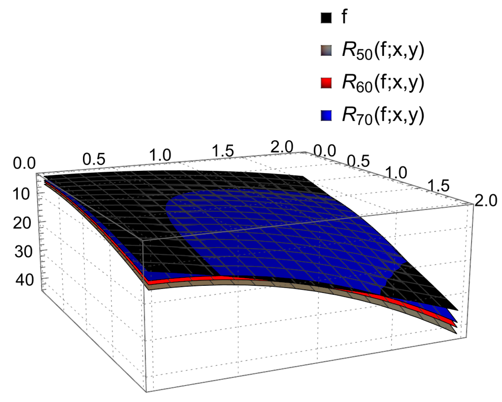
7. Numerical and Graphical Analyses of Bivariate Operators

We present graphical and numerical analyses of the bivariate operators defined in (13) to demonstrate their convergence. Using the test function $f(x,y)=2{(x+y)}^2+4$, the convergence behavior is illustrated in Figure 3. To examine the error approximation, we employ the formula $S_{n,m}(f;x,y)=\left|R_{n,m}(f;x,y)-f(x,y)\right|$, analyzing the error for different values of n and m, specifically $n,m=50,60,$ and 70. The corresponding error approximations are graphically represented in Figure 4 and numerically tabulated in

Table 2. Error approximation table: $S_{n,m}(f;x,y)=\left|R_{n,m}(f;x,y)-f(x,y)\right|$.

$\mathit{x},\mathit{y}$	${\mathit{S}}_{50,50}(\mathit{f};\mathit{x},\mathit{y})$	${\mathit{S}}_{60,60}(\mathit{f};\mathit{x},\mathit{y})$	${\mathit{S}}_{70,70}(\mathit{f};\mathit{x},\mathit{y})$
0.2, 0.2	2.59048	1.80191	1.210319
0.4, 0.4	2.27578	1.45012	0.829109
0.6, 0.6	1.81534	0.927824	0.257771
0.8, 0.8	1.30501	0.331003	0.407696
1.0, 1.0	0.87933	0.205938	1.032911
1.2, 1.2	0.71105	0.510199	1.44504
1.4, 1.4	1.01139	0.370581	1.432913
1.6, 1.6	2.02992	0.462517	0.746917
1.8, 1.8	4.05466	2.277118	0.900942

. Collectively, the figures and the table provide insights into the behavior and accuracy of the operator as n and m increase, confirming its convergence to the target function $f(x,y)$.

8. Conclusions

In this study, we explored the approximation capabilities of Frobenius–Euler–Simsek polynomials analogous to Szász–Kantorovich operators for Lebesgue measurable functions. Through extensive testing and calculation of the test functions and central moments, we analyzed their uniform convergence and order of approximation. Our investigation included the Korovkin theorem and the modulus of continuity, assessing how well these operators approximated the functions within continuous functional spaces. We also examined Voronovskaja-type theorems for functions with continuous derivatives, supported by numerical and graphical analyses of the errors. Additionally, we developed a bivariate sequence of operators for approximating bivariate continuous functions, discussing the numerical and graphical error deviations.

References

1. Bernstein, S.N. Démonstration du théorème de Weierstrass fondée sur le calcul de probabilités. Commun. Soc. Math. Kharkow. 1913, 13, 1–2. [Google Scholar]
2. Weierstrass, K. Über die analytische Darstellbarkeit sogenannter willkürlicher Functionen einer reellen Veränderlichen. Sitzungsberichte KöNiglichen PreußIschen Akad. Wiss. Berl. 1885, 2, 633–639. [Google Scholar]
3. Kantorovich, L.V. Sur certain developpments suivant les polynomes de la forme de S. Bernstein, I, II. C. R. Acad. URSS 1930, 563–568, 595–600. [Google Scholar]
4. Khan, K.; Lobiyal, D.K. Bézier curves based on Lupăs (p,q)-analogue of Bernstein functions in CAGD. Comput. Appl. Math. 2017, 317, 458–477. [Google Scholar] [CrossRef]
5. Raiz, M.; Rao, N.; Mishra, V.N. Szász-type operators involving q-Appell polynomials. In Approximation Theory, Sequence Spaces and Applications; Mohiuddine, S.A., Hazarika, B., Nashine, H.K., Eds.; Industrial and Applied Mathematics; Springer: Singapore, 2022. [Google Scholar] [CrossRef]
6. Khan, K.; Lobiyal, D.K.; Kilicman, A. Bézier curves and surfaces based on modified Bernstein polynomials. Azerb. J. Math. 2019, 9, 102–115. [Google Scholar]
7. Izadbakhsh, A.; Kalat, A.A.; Khorashadizadeh, S. Observer-based adaptive control for HIV infection therapy using the Baskakov operator. Biomed. Signal Process. Control 2021, 65, 102343. [Google Scholar] [CrossRef]
8. Uyan, H.; Aslan, A.O.; Karateke, S.; Büyükyazıcı, İ. Interpolation for neural network operators activated with a generalized logistic-type function. Neural Comput. Appl. 2024, in press. [CrossRef]
9. Zhang, Q.; Mu, M.; Wang, X. A modified robotic manipulator controller based on Bernstein-Kantorovich-Stancu operator. Micromachines 2022, 14, 44. [Google Scholar] [CrossRef]
10. Özger, F. Weighted statistical approximation properties of univariate and bivariate λ-Kantorovich operators. Filomat 2019, 33, 3473–3486. [Google Scholar] [CrossRef]
11. Özger, F.; Ansari, K.J. Statistical convergence of bivariate generalized Bernstein operators via four-dimensional infinite matrices. Filomat 2022, 36, 543–555. [Google Scholar] [CrossRef]
12. Cai, Q.B.; Lian, B.Y.; Zhou, G. Approximation properties of λ-Bernstein operators. J. Inequal. Appl. 2018, 2018, 61. [Google Scholar] [CrossRef] [PubMed]
13. Cai, Q.B.; Zhou, G.; Li, J. Statistical approximation properties of λ-Bernstein operators based on q-integers. Open Math. 2019, 17, 487–498. [Google Scholar]
14. Aslan, R. Rate of approximation of blending type modified univariate and bivariate λ-Schurer-Kantorovich operators. Kuwait J. Sci. 2024, 51, 100168. [Google Scholar]
15. Aslan, R. Approximation properties of univariate and bivariate new class-Bernstein–Kantorovich operators and its associated GBS operators. Comput. Appl. Math. 2023, 42, 34. [Google Scholar] [CrossRef]
16. Acu, A.M.; Gonska, H.; Rașa, I. Grüss-type and Ostrowski-type inequalities in approximation theory. Ukr. Math. J. 2011, 63, 843–864. [Google Scholar]
17. Acu, A.M.; Acar, T.; Radu, V.A. Approximation by modified U n ρ operators. Rev. R. Acad. Cienc. Exactas Fís. Nat. Ser. A Math. 2019, 113, 2715–2729. [Google Scholar]
18. Acu, A.M.; Tachev, G. Yet another new variant of Szász–Mirakyan operator. Symmetry 2021, 13, 2018. [Google Scholar] [CrossRef]
19. Mohiuddine, S.A.; Acar, T.; Alotaibi, A. Construction of a new family of Bernstein-Kantorovich operators. Math. Methods Appl. Sci. 2017, 40, 7749–7759. [Google Scholar]
20. Mohiuddine, S.A.; Ahmad, N.; Özger, F.; Alotaibi, A.; Hazarika, B. Approximation by the parametric generalization of Baskakov–Kantorovich operators linking with Stancu operators. Iran. J. Sci. Technol. Trans. A Math. 2021, 45, 593–605. [Google Scholar] [CrossRef]
21. Mursaleen, M.; Ansari, K.J.; Khan, A. Approximation properties and error estimation of q-Bernstein shifted operators. Numer. Algorithms 2020, 84, 207–227. [Google Scholar] [CrossRef]
22. Mursaleen, M.; Naaz, A.; Khan, A. Improved approximation and error estimations by King type (p, q)-Szász–Mirakjan Kantorovich operators. Appl. Math. Comput. 2019, 348, 2175–2185. [Google Scholar]
23. Bustamante, J. Direct estimates and a Voronovskaja-type formula for Mihesan operators. Comput. Math. Appl. 2022, 5, 202–213. [Google Scholar]
24. Ozsarac, F.; Gupta, V.; Aral, A. Approximation by some Baskakov–Kantorovich exponential-type operators. Bull. Iran. Math. Soc. 2022, 48, 227–241. [Google Scholar]
25. Khan, A.; Mansoori, M.; Khan, K.; Mursaleen, M. Phillips-type q-Bernstein operators on triangles. J. Funct. Spaces 2021, 1–13. [Google Scholar] [CrossRef]
26. Nasiruzzaman, M. Approximation properties by Szász–Mirakjan operators to bivariate functions via Dunkl analogue. Iran. J. Sci. Technol. Trans. A Math. 2011, 45, 259–269. [Google Scholar]
27. Braha, N.L.; Loku, V.; Mansour, T.; Mursaleen, M. A new weighted statistical convergence and some associated approximation theorems. Math. Methods Appl. Sci. 2022, 45, 5682–5698. [Google Scholar]
28. Rao, N.; Farid, M.; Ali, R.A. Study of Szász–Durremeyer-Type Operators Involving Adjoint Bernoulli Polynomials. Mathematics 2024, 12, 3645. [Google Scholar] [CrossRef]
29. Rao, N.; Farid, M.; Raiz, M. Symmetric Properties of λ-Szász Operators Coupled with Generalized Beta Functions and Approximation Theory. Symmetry 2024, 16, 1703. [Google Scholar] [CrossRef]
30. Çetin, N. Approximation and geometric properties of complex α-Bernstein operator. Results Math. 2019, 74, 40. [Google Scholar]
31. Çetin, N.; Radu, V.A. Approximation by generalized Bernstein–Stancu operators. Turk. J. Math. 2019, 43, 2032–2048. [Google Scholar]
32. Simsek, Y. Applications of constructed new families of generating-type functions interpolating new and known classes of polynomials and numbers. Math. Methods Appl. Sci. 2021, 44, 11245–11268. [Google Scholar] [CrossRef]
33. Kucukoglu, I. Generating functions for multiparametric Hermite-based Peters-type Simsek numbers and polynomials in several variables. Montes Taurus J. Pure Appl. Math. 2024, 6, 217–238. [Google Scholar]
34. Kucukoglu, I.; Simsek, Y. Identities and relations on the q-Apostol type Frobenius–Euler numbers and polynomials. J. Korean Math. Soc. 2019, 56, 265–284. [Google Scholar]
35. Agyuz, E. On the convergence properties of generalized Szász–Kantorovich type operators involving Frobenius–Euler–Simsek-type polynomials. AIMS Math. 2024, 9, 28195–28210. [Google Scholar]
36. DeVore, R.A.; Lorentz, G.G. Constructive Approximation; Springer: Berlin/Heidelberg, Germany, 1993. [Google Scholar]
37. Altomare, F.; Campiti, M. Korovkin-Type Approximation Theory and Its Applications; De Gruyter Studies in Mathematics; De Gruyter: Berlin, Germany, 1994; Volume 17, pp. 266–274. [Google Scholar]
38. Özarslan, M.A.; Aktuğlu, H. Local approximation for certain King type operators. Filomat 2013, 27, 173–181. [Google Scholar]
39. Volkov, V.I. On the convergence of sequences of linear positive operators in the space of continuous functions of two variables. Dokl. Akad. Nauk SSSR (NS) 1957, 115, 17–19. (In Russian) [Google Scholar]
40. Stancu, F. Aproximarea Funcţiilor de Două şi Mai Multe Variabile Prin şIruri de Operatori Liniari şi Pozitivi. Ph.D. Thesis, University ”Babe¸s-Bolyai”, Cluj-Napoca, Romania, 1984. (In Russian). [Google Scholar]
Figure 1. Convergence of operator K n ( f ; y ) for n = 50 , 60 , 70 .
Axioms 14 00252 g001
Figure 2. Error approximation E n ( f ; y ) = K n ( f ; y ) f ( y ) .
Axioms 14 00252 g002
Figure 3. Convergence of the operator K n , m ( f ; x , y ) for n = m = 50 , 60 , 70 .
Axioms 14 00252 g003
Figure 4. Error approximation S n , m ( f ; x , y ) = R n , m ( f ; x , y ) f ( x , y ) .
Axioms 14 00252 g004