Circuit Design and Implementation of a Time-Varying Fractional-Order Chaotic System

Abstract

This paper presents a circuit design methodology for the analog realization of time-varying fractional-order chaotic systems. While most existing studies implement such systems by switching between two or more constant fractional orders, these approaches become impractical when the fractional order changes smoothly over time. To overcome this limitation, the proposed method introduces a transfer function approximation specifically designed for variable fractional-order integrators. The formulation relies on a linear and time-invariant definition of the fractional-order operator, ensuring compatibility with Laplace-domain analysis. Under the condition that the fractional-order function is Laplace-transformable and its Bode plot slope lies between $-20$ dB/decade and 0 dB/decade, the system is realized using op-amps and standard RC components. The Grünwald–Letnikov method is employed for numerical calculation of phase portraits, which are then compared with simulation and experimental results. The strong agreement among these results confirms the effectiveness of the proposed method.

1. Introduction

Chaos and chaos-based applications have become topical subjects across various fields of study in the literature. Chaos is utilized in numerous areas, including data security [1,2], random number generation [3,4], optimization [5,6], control [7,8], communication [9,10], biology [11,12], economics [13,14], and so on.

When chaos, as a science subject, was first introduced by Lorenz [15], the chaotic system consisted of integer-order differential equations. Later, constant fractional-order chaotic systems were favored because of their higher nonlinear property and more complex dynamic behavior. In [16], the hidden dynamics of the attractors are explored for various fractional orders, a phenomenon not observed in the integer order. Moreover, fractional-order systems have an advantage over integer-order systems in terms of defining the long memory of the systems [17,18,19,20]. In some real-world problems, fractal–fractional-order operators may yield a more accurate result than integer-order operators [21,22].

However, some studies [23,24,25,26] suggest that certain systems or applications need memory to be changed with time or space. This cannot be defined with the constant fractional-order case; thus, variable fractional-order systems are developed [26]. In the literature, various approaches have been proposed to define variable fractional-order integro-differential operators, tailored to specific applications [23,27,28].

In most studies, the analog realization of integer- or fractional-order chaotic systems via electronic circuits is carried out as modeling of the chaotic system in a real environment [27,28,29,30,31,32,33,34,35]. In the constant fractional-order case, the transfer function is approximated by the fractional power pole method introduced by Charef et al. [36]. After obtaining the approximated transfer function, the fractional-order integrator is designed using different circuit synthesizing methods, such as an RC chain, tree, or ladder structure [32].

For the variable fractional-order case, the circuit realization is carried out with switching techniques, described in [23]. In [27,28,31], the variable fractional-order integrator is realized using switches in which the variable fractional order has two or three different constant values. However, this approach is not practical when the fractional order varies continuously over time.

In this paper, a method is proposed for approximating the transfer function of a time-varying fractional-order integrator. While several techniques exist in the literature for the approximation of constant fractional-order systems—such as the approach detailed in [36]—these methods are not directly applicable when the fractional order varies continuously with time. To the best of the author’s knowledge, this study presents the first successful realization of a variable fractional-order chaotic system using such an approximation framework. The method introduced here represents the core contribution of this work and offers a practical foundation for analog implementation of variable-order dynamics.

However, the proposed method has certain limitations. First, since the approach relies on approximating the transfer function of the variable fractional-order integrator, the definition of variable fractional-order integration must be linear and time-invariant. Only the third definition given in [23] is linear and time-invariant, so the proposed method can be only used for this definition. Second, the variable fractional order must be Laplace-transformable. Finally, the slope of the variable fractional-order integrator must vary between $-20$ dB/decade and 0 dB/decade over the frequency range of interest, since the transfer function is approximated with zig-zag lines with slopes of $-20$ dB/decade and 0 dB/decade.

The structure of the paper is as follows: Section 2 introduces variable fractional-order operators, Section 3 outlines circuit design steps for variable fractional-order integrators, Section 4 presents the variable fractional-order chaotic system used in this study, Section 5 provides an example implementation of the variable fractional-order chaotic system, and Section 6 offers the conclusion.

2. Variable Fractional-Order Operators

This section provides the definition of fractional-order operators and explains how time-varying fractional orders are defined. In the literature, there are different definitions of fractional-order derivatives or integrals. In this paper, the Riemann–Liouville (RL) definition is considered for the fractional-order integrator. For numerical calculation, the Grünwald–Letnikov (GL) fractional order definition is employed, since the finite difference-based definition of GL is equivalent to the RL definition [37,38].

The Riemann–Liouville definition for the constant fractional-order integral is [39,40]

$${}_{0}D_t^{-q}x\left(t\right)={\int }_0^t{\displaystyle \frac{{(t-\tau )}^{q-1}}{\Gamma \left(q\right)}}x\left(\tau \right)d\tau .$$

(1)

Then, the constant fractional-order Grünwald–Letnikov fractional derivative is [41,42]

$${}_{0}D_t^{q}x\left(t\right)=\underset{h\to 0}{lim}{h}^{-q}\sum _{i=0}^{{\displaystyle \frac{t}{h}}}{(-1)}^i\left({\displaystyle \genfrac{}{}{0pt}{}{q}{i}}\right)x(t-ih).$$

(2)

Here, $x\left(t\right)$ is the differentiable function, q is the fractional order, h is the step size, and $\left({\displaystyle \genfrac{}{}{0pt}{}{q}{i}}\right)$ is the binomial coefficients, where

$$\left({\displaystyle \genfrac{}{}{0pt}{}{q}{i}}\right)=\left\{\begin{array}{c}1\mathrm{for}i=0,\hfill \\ {\displaystyle \frac{q(q-1)\dots (q-i+1)}{i!}}\mathrm{for}i>0.\hfill \end{array}\right.$$

(3)

Formula (2) can be used for the Grünwald–Letnikov fractional-order integral when $q<0$ [43]; then, the fractional-order integral is

$${}_{0}D_t^{-q}x\left(t\right)=\underset{h\to 0}{lim}{h}^q\sum _{i=0}^{{\displaystyle \frac{t}{h}}}{(-1)}^i\left({\displaystyle \genfrac{}{}{0pt}{}{-q}{i}}\right)x(t-ih).$$

(4)

This equation can be used for the constant-order case. Next, the variable-order case is considered. In the literature, there are many different approaches for defining variable-order fractional integro-differential operators. Lorenzo and Hartley [23] considered three different cases of how to handle time-varying orders. In [23], the Riemann–Liouville definition for the fractional-order integral is employed.

The general Riemann–Liouville definition of the time-varying fractional order integral [23] is

$${}_{0}D_t^{-q\left(t\right)}x\left(t\right)={\int }_0^t{\displaystyle \frac{{(t-\tau )}^{q(t,\tau )-1}}{\Gamma \left(q\right(t,\tau \left)\right)}}x\left(\tau \right)d\tau .$$

(5)

Different definitions for the variable fractional-order case are derived according to the definition of $q(t,\tau )$.

In the third case in [23], the time-varying order in (5) is defined as $q(t,\tau )=q(t-\tau )$. Under this definition, the time-varying fractional-order integral is expressed as

$${}_{0}D_t^{-q\left(t\right)}x\left(t\right)={\int }_0^t{\displaystyle \frac{{(t-\tau )}^{q(t-\tau )-1}}{\Gamma \left(q\right(t-\tau \left)\right)}}x\left(\tau \right)d\tau .$$

(6)

This type of integral is time-invariant and strongly remembers past values of variable order q [23]. Due to its time-invariant property, this definition is adopted for the circuit implementation presented in this paper. In this case, the time-varying integral can be represented in the Laplace domain as follows [23]:

$$L\left\{{}_{0}D_t^{-q\left(t\right)}x\left(t\right)\right\}=s^{-sL\left\{q\left(t\right)\right\}}X\left(s\right).$$

(7)

Formula (7) will be used in the approximation of the circuit implementation of the variable-order chaotic system, which will be discussed in Section 3.

For the numeric calculation, the Grünwald–Letnikov definition, which is equivalent to (6), is used as given in (8) [44,45]:

$${}_{0}D_t^{-q\left(t\right)}x\left(t\right)=\underset{h\to 0}{lim}\sum _{i=0}^{{\displaystyle \frac{t}{h}}}{h^{q\left(i\right)}(-1)}^i\left({\displaystyle \genfrac{}{}{0pt}{}{-q\left(i\right)}{i}}\right)x(t-ih).$$

(8)

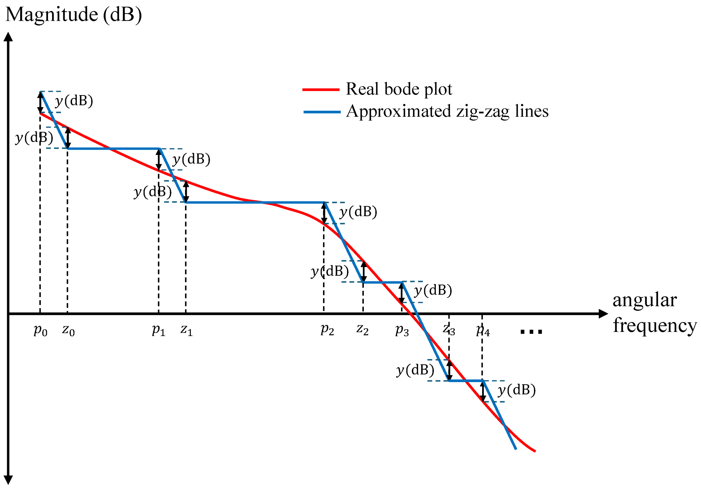
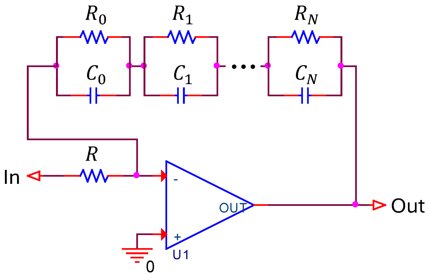
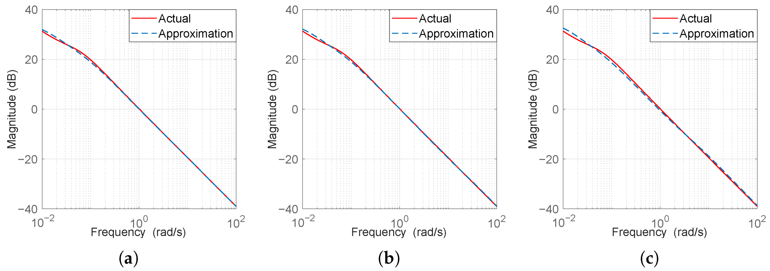
3. Circuit Design Steps for Variable Fractional-Order Integrator

In this section, the circuit design procedure is explained. Most studies in the literature [29,30,32,46] use the fractional power pole method to define the transfer function of constant fractional-order integrator circuits. In the constant fractional-order integrator, the transfer function is  

$$H\left(s\right)={\displaystyle \frac{1}{s^q}},$$

(9)

where q is the constant fractional order. This transfer function can be approximated by employing a fractional power pole, as described in [36]

$${\displaystyle \frac{1}{s^q}}\approx {\displaystyle \frac{1}{{\left(1+\frac{s}{p_t}\right)}^q}}.$$

(10)

Here, $p_t$ is the corner frequency (and $1/p_t$ is the relaxation time). Then, the approximation of the fractional power pole is [36]

$${\displaystyle \frac{1}{{\left(1+\frac{s}{p_t}\right)}^q}}\cong {\displaystyle \frac{{\prod }_{n=0}^{N-1}\left(1+\frac{s}{z_i}\right)}{{\prod }_{n=0}^N\left(1+\frac{s}{p_i}\right)}}.$$

(11)

Here, the value of N depends on the frequency range of interest. In this method, the fractional power pole is approximated by employing a pole–zero pair. In other words, the Bode diagram of ${\displaystyle \frac{1}{{(1+\frac{s}{p_t})}^q}}$ is approximated with zig-zag lines with slopes of $-20$ dB/dec and 0 dB/dec.

The Bode plots of both ${\displaystyle \frac{1}{s^q}}$ and ${\displaystyle \frac{1}{{(1+\frac{s}{p_t})}^q}}$ have a slope of $-20q$ dB/decade; however their magnitudes differ. The amplitude of the transfer function of the fractional-order integrator is

$$\left|{\displaystyle \frac{1}{s^q}}\right|={\displaystyle \frac{1}{{\left|s\right|}^q}},$$

(12)

and the amplitude of the fractional power pole is

$$\left|{\displaystyle \frac{1}{{\left(1+\frac{s}{p_t}\right)}^q}}\right|=\left|{\displaystyle \frac{p_t^q}{{\left(p_t+s\right)}^q}}\right|\cong p_t^q{\displaystyle \frac{1}{{\left|s\right|}^q}},\mathrm{for}s\gg p_t.$$

(13)

Since both Bode plots have the exact same slope, the difference in the magnitudes is compensated by multiplying the latter one with a gain of ${\displaystyle \frac{1}{p_t^q}}$. Therefore, the approximated transfer function of the constant-order integrator becomes

$${\displaystyle \frac{1}{s^q}}\cong {\displaystyle \frac{1}{p_t^q}}{\displaystyle \frac{1}{{\left(1+\frac{s}{p_t}\right)}^q}}\cong {\displaystyle \frac{1}{p_t^q}}{\displaystyle \frac{{\prod }_{n=0}^{N-1}\left(1+\frac{s}{z_i}\right)}{{\prod }_{n=0}^N\left(1+\frac{s}{p_i}\right)}}.$$

(14)

How the value of poles ($p_i$) and zeros ($z_i$) is calculated is given in [36].

For the variable fractional-order integrator, the transfer function can be written as

$$H\left(s\right)={\displaystyle \frac{1}{s^{sQ\left(s\right)}}}.$$

(15)

Here, $Q\left(s\right)$ is the Laplace transform of the variable order $q\left(t\right)$ (i.e., $Q\left(s\right)=Lq\left(t\right)$). For the approximation of (14), the procedure explained in [36] cannot be used directly since the slopes of ${\displaystyle \frac{1}{s^{sQ\left(s\right)}}}$ and ${\displaystyle \frac{1}{{(1+\frac{s}{p_t})}^{sQ\left(s\right)}}}$ are not the same for the entire frequency range since the magnitude of ${\displaystyle \frac{1}{p_t^{sQ\left(s\right)}}}$ is a function of frequency. However, a similar approach will be used to approximate the transfer function in (15). Instead of using a fractional power pole, the Bode plot of (15) will be directly used to approximate it with zig-zag lines with slopes of $-20$ dB/dec and 0 dB/dec.

In Figure 1, the Bode plot of a variable fractional-order integrator and its approximation with zig-zag lines are shown. The zig-zag lines have alternating slopes of $-20$ dB/dec and 0 dB/dec. As seen in the figure, the approximated transfer function’s lowest and highest singularities are poles. Hence, the approximated transfer function has N zeros and $N+1$ poles. Then, the approximation for the variable fractional-order case is

$${\displaystyle \frac{1}{s^{sQ\left(s\right)}}}\approx {\displaystyle \frac{{\prod }_{n=0}^{N-1}\left(1+\frac{s}{z_i}\right)}{{\prod }_{n=0}^N\left(1+\frac{s}{p_i}\right)}}.$$

(16)

This result is the same as the constant fractional-order case; however, the method used to compute the pole–zero values in the constant-order case [36] is not applicable in the variable-order scenario. For the variable-order case, the calculation of pole–zero values is given in (19).

The right-hand side of (16) exhibits an amplitude of 0 dB at the frequency $p_0$. However, this value must be y dB higher than the Bode plot magnitude of the variable-order integrator at the same frequency. This discrepancy can be effectively compensated by introducing an appropriate gain correction term. Then, the approximated transfer function becomes

$$H\left(s\right)={\displaystyle \frac{1}{s^{sQ\left(s\right)}}}\cong k{\displaystyle \frac{{\prod }_{n=0}^{N-1}\left(1+\frac{s}{z_i}\right)}{{\prod }_{n=0}^N\left(1+\frac{s}{p_i}\right)}},$$

(17)

and the gain k is calculated as

$$k={{10}^{y/20}\left.{\displaystyle \frac{\left|\frac{1}{s^{sQ\left(s\right)}}\right|}{1/\left|1+\frac{s}{p_0}\right|}}\right|}_{s=j{p}_o}.$$

(18)

To approximate the variable fractional-order integrator, the first step is to determine the frequency band of interest. The first pole $p_0$ corresponds to the start frequency, while the last pole $p_N$ is greater than or equal to the stop frequency of the band. In this way, the approximated transfer function has N zeros and $N+1$ poles.

Then, for the calculation of the other pole-and-zero pairs, the following equations must be solved.

$$\begin{array}{cc}\hfill & {\displaystyle \frac{{\left.\left|\frac{1}{s^{sQ\left(s\right)}}\right|\right|}_{s=j{z}_0}}{k{\left.\left|\frac{1}{s/p_0}\right|\right|}_{s=j{z}_0}}}-{10}^{{\displaystyle \frac{y}{20}}}=0\left(for{z}_o\right),\hfill \\ \hfill & {\displaystyle \frac{k\left|\frac{1/z_0}{1/p_0}\right|}{{\left.\left|\frac{1}{s^{sQ\left(s\right)}}\right|\right|}_{s=j{p}_1}}}-{10}^{{\displaystyle \frac{y}{20}}}=0\left(for{p}_1\right),\hfill \\ \hfill & {\displaystyle \frac{{\left.\left|\frac{1}{s^{sQ\left(s\right)}}\right|\right|}_{s=j{z}_1}}{k{\left.\left|\frac{1/z_0}{s(1/p_0)(1/p_1)}\right|\right|}_{s=j{z}_1}}}-{10}^{{\displaystyle \frac{y}{20}}}=0\left(for{z}_1\right),\hfill \\ \hfill & {\displaystyle \frac{k\left|\frac{(1/z_0)(1/z_1)}{(1/p_0)(1/p_1)}\right|}{{\left.\left|\frac{1}{s^{sQ\left(s\right)}}\right|\right|}_{s=j{p}_2}}}-{10}^{{\displaystyle \frac{y}{20}}}=0\left(for{p}_2\right),\hfill \\ \hfill & ⋮\hfill \\ \hfill & {\displaystyle \frac{k\left|\frac{{\prod }_{i=0}^{n-1}(1/z_i)}{{\prod }_{i=0}^{n-1}(1/p_i)}\right|}{{\left.\left|\frac{1}{s^{sQ\left(s\right)}}\right|\right|}_{s=j{p}_n}}}-{10}^{{\displaystyle \frac{y}{20}}}=0\left(for{p}_n\right),\hfill \\ \hfill & {\displaystyle \frac{{\left.\left|\frac{1}{s^{sQ\left(s\right)}}\right|\right|}_{s=j{z}_n}}{k{\left.\left|\frac{{\prod }_{i=0}^{n-1}(1/z_i)}{s{\prod }_{i=0}^n(1/p_i)}\right|\right|}_{s=j{z}_n}}}-{10}^{{\displaystyle \frac{y}{20}}}=0\left(for{z}_n\right),\hfill \\ \hfill & ⋮\hfill \\ \hfill & {\displaystyle \frac{{\left.\left|\frac{1}{s^{sQ\left(s\right)}}\right|\right|}_{s=j{z}_{N-1}}}{k{\left.\left|\frac{{\prod }_{i=0}^{N-2}(s/z_i)}{{\prod }_{i=0}^{N-1}(s/p_i)}\right|\right|}_{s=j{z}_{N-1}}}}-{10}^{{\displaystyle \frac{y}{20}}}=0\left(for{z}_{N-1}\right),\hfill \\ \hfill & {\displaystyle \frac{k{\left.\left|\frac{{\prod }_{i=0}^{N-1}(s/z_i)}{{\prod }_{i=0}^{N-1}(s/p_i)}\right|\right|}_{s=j{p}_N}}{{\left.\left|\frac{1}{s^{sQ\left(s\right)}}\right|\right|}_{s=j{p}_N}}}-{10}^{{\displaystyle \frac{y}{20}}}=0\left(for{p}_N\right).\hfill \end{array}$$

(19)

Obtaining analytical solutions to the equations in (19) is not straightforward. However, these solutions can be easily obtained graphically. The values of zeros ($z_i$) or poles ($p_i$) can be obtained by plotting the left-hand sides of the equations with respect to the frequency range of the interest. Here, the complex variable s must be substituted with $j\omega$. The points where these plots cross the zero axis correspond to the solutions of the equations. These pole–zero pairs are calculated iteratively until the last pole, $p_N$, is greater than or equal to the highest-frequency term in the frequency band. A simple algorithm for calculating poles and zeros is provided in Algorithm 1.

After the poles and zeros are obtained, the variable fractional-order integrator is realized with an op-amp and RC tank network, as shown in Figure 2. In the circuit, the value of resistors and capacitors are dependent on the transfer function and hence on the value of poles and zeros.

If the circuit analysis is performed for the fractional-order integrator given in Figure 2, the transfer function is obtained as follows:

$${\displaystyle \frac{V_{out}}{V_{In}}}=-{\displaystyle \frac{\frac{1/C_0}{s+1/R_0{C}_0}+\frac{1/C_1}{s+1/R_1{C}_1}+\dots +\frac{1/C_N}{s+1/R_N{C}_N}}{R}}.$$

(20)

Algorithm 1 The pseudo code for calculation of pole–zero of the approximated transfer function.

Determining the frequency range of approximation [${\omega }_1,{\omega }_2$] $p_0\leftarrow {\omega }_1$ Setting the maximum error y $k\leftarrow {{10}^{y/20}\left.{\displaystyle \frac{\left|\frac{1}{s^{sQ\left(s\right)}}\right|}{1/\left|1+\frac{s}{p_0}\right|}}\right|}_{s=j{p}_o}$ while $p_n\le {\omega }_2$ do     $z_{n-1}\leftarrow zerocrossingof{\displaystyle \frac{{\left.\left|\frac{1}{s^{sQ\left(s\right)}}\right|\right|}_{s=j\omega }}{k{\left.\left|\frac{{\prod }_{i=0}^{n-2}(1/z_i)}{s{\prod }_{i=0}^{n-1}(1/p_i)}\right|\right|}_{s=j\omega }}}-{10}^{{\displaystyle \frac{y}{20}}}$     $p_n\leftarrow zerocrossingof{\displaystyle \frac{k\left|\frac{{\prod }_{i=0}^{n-1}(1/z_i)}{{\prod }_{i=0}^{n-1}(1/p_i)}\right|}{{\left.\left|\frac{1}{s^{sQ\left(s\right)}}\right|\right|}_{s=j\omega }}}-{10}^{{\displaystyle \frac{y}{20}}}$     $n\leftarrow n+1$ end while

In (20), drop the negative sign for further analysis, since the negative sign can be easily gotten rid of by an inverting amplifier. Moreover, set the value of the input-side resistance R as 1 $\Omega$. In this way, the transfer function given in (20) becomes

$${\displaystyle \frac{1/C_0}{s+1/R_0{C}_0}}+{\displaystyle \frac{1/C_1}{s+1/R_1{C}_1}}+\dots +{\displaystyle \frac{1/C_N}{s+1/R_N{C}_N}}.$$

(21)

Now, this transfer function can be used to approximate the variable-order integrator. The transfer function in (17) can be rewritten as

$$H\left(s\right)={\displaystyle \frac{1}{s^{sQ\left(s\right)}}}\cong k{\displaystyle \frac{{\prod }_{n=0}^{N-1}\left(1+\frac{s}{z_i}\right)}{{\prod }_{n=0}^N\left(1+\frac{s}{p_i}\right)}}=a{\displaystyle \frac{{\prod }_{n=0}^{N-1}\left(1+\frac{s}{z_i}\right)}{\left(s+p_o\right)\left(s+p_1\right)\dots (s+p_N)}}.$$

(22)

Then, partial fraction expansion is applied to the right-hand side of (22):

$$a{\displaystyle \frac{{\prod }_{n=0}^{N-1}\left(1+\frac{s}{z_i}\right)}{\left(s+p_o\right)\left(s+p_1\right)\dots (s+p_N)}}={\displaystyle \frac{r_0}{s+p_0}}+{\displaystyle \frac{r_1}{s+p_1}}+\dots +{\displaystyle \frac{r_N}{s+p_N}}.$$

(23)

Here, all the residues are positive constants since the poles and zeros are alternate in order. Hence, the transfer function in (17) can be realized using passive elements such as resistors and capacitors. The value of the resistors and capacitors is calculated as

$$\begin{array}{cc}\hfill & C_i={\displaystyle \frac{1}{r_i}},\hfill \\ \hfill & R_i={\displaystyle \frac{r_i}{p_i}}.\hfill \end{array}$$

(24)

After all the values of $R_i$ and $C_i$ are calculated, the magnitude scaling process can be performed on the integrator circuit in Figure 2 to shift the values of $R,R_i$, and $C_i$ to a more practical range. Magnitude scaling in a network is scaling up/down all the impedances in the network by the same factor; hence, the process does not change the transfer function. Moreover, the frequency scaling process may be applied to the integrator circuit in Figure 2 to shift its frequency spectrum. An example of a circuit implementation of a variable fractional-order chaotic system is given in Section 5.

As a final remark, the fractional variable order and its Bode plot must meet the following criteria for the described circuit design steps to be applicable. The variable fractional order $q\left(t\right)$ must vary between 0 and 1 and also have a Laplace transform. The slope of the Bode plot of $q\left(t\right)$ must vary between $-20$ dB/dec and 0 dB/dec in the frequency range of interest.

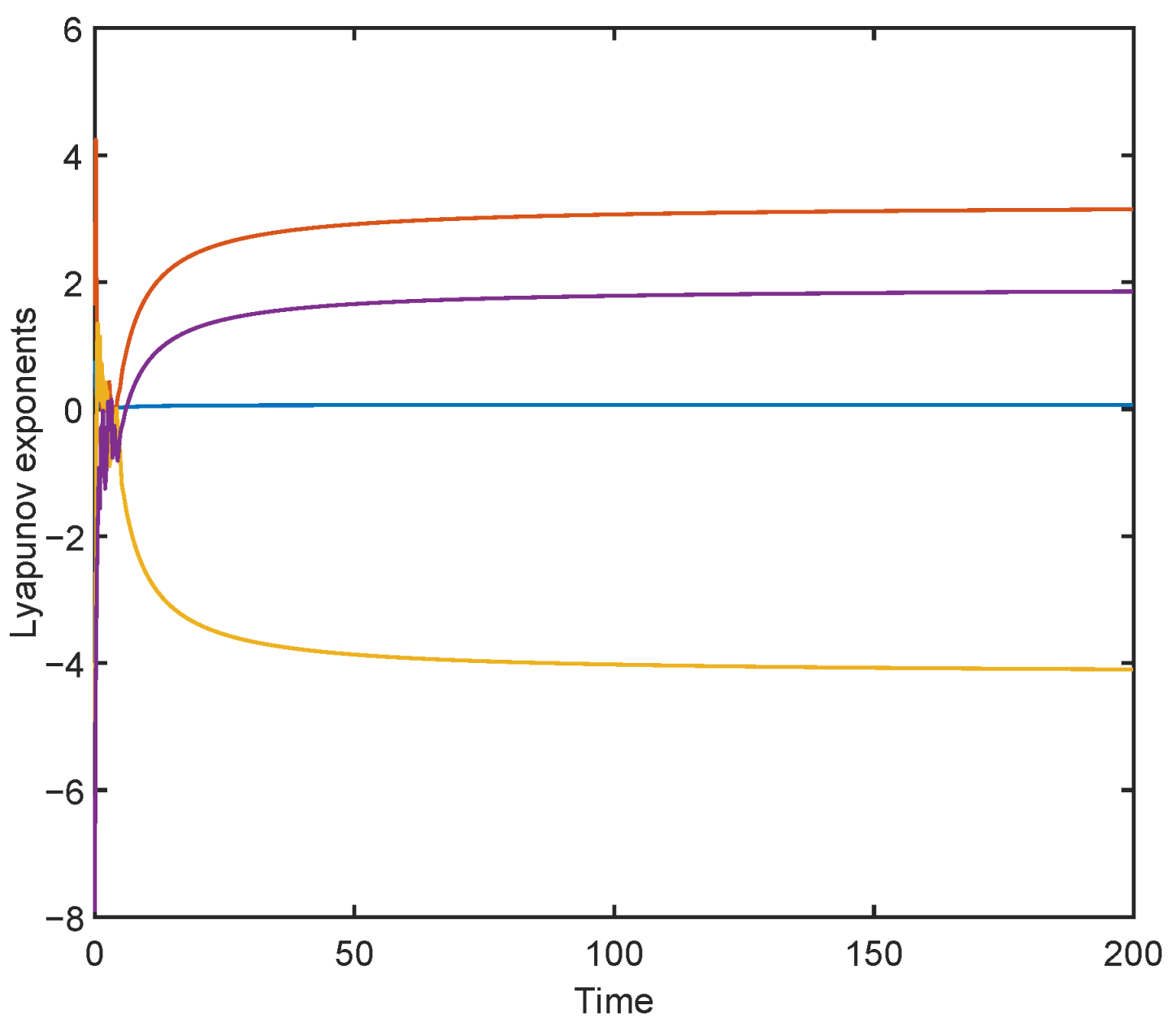
4. Variable Fractional-Order Chaotic System

In this section, the variable fractional-order chaotic system used in this study is introduced. The chaotic system is a four-dimensional system that is derived from a physical system, as described in [47]. In [47], the chaotic system is an integer order, whereas in this paper the order of the chaotic system is time-varying. The main reason for selecting this system is that it can exhibit chaotic behavior even when all the initial values of the state variables are zero. This property makes the circuit implementation easier. The variable fractional-order chaotic system is given in (25).

$$\begin{array}{cc}\hfill & {\displaystyle \frac{d^{q\left(t\right)}x}{d{t}^{q\left(t\right)}}}=z,\hfill \\ \hfill & {\displaystyle \frac{d^{q\left(t\right)}y}{d{t}^{q\left(t\right)}}}=w,\hfill \\ \hfill & {\displaystyle \frac{d^{q\left(t\right)}z}{d{t}^{q\left(t\right)}}}=-\alpha z-\beta x-\rho {(x-y)}^2,\hfill \\ \hfill & {\displaystyle \frac{d^{q\left(t\right)}w}{d{t}^{q\left(t\right)}}}=\gamma -\sigma w-\zeta {(y-x)}^2.\hfill \end{array}$$

(25)

Here, the time-varying fractional order is defined as $q\left(t\right)=0.76+0.215e^{-0.05t}$, the values of the parameters are selected as $\alpha =1.1,\beta =12,\rho =25,\gamma =1.25,\sigma =7.5$, and $\zeta =25$, and the initial conditions are $x_0=y_0=z_0=w_0=0$.

In this section, all numerical computations are carried out using MATLAB 9.4. The phase portraits are generated by solving the time-varying fractional-order system defined in (8), while the bifurcation diagram and Lyapunov exponent analysis are performed using the algorithms presented in [48] and [49], respectively.

The Lyapunov exponent spectra and bifurcation diagram are given in Figure 3, Figure 4 and Figure 5 to show that the system exhibits chaotic behavior.

Figure 4 presents the Lyapunov spectra of the variable fractional-order system with respect to each system parameter. During the analysis, a parametric sweep is conducted by varying one parameter at a time, while all other parameters are held constant to show the individual effects of each parameter on system dynamics.

Moreover, the 0–1 test for chaos is employed to investigate the dynamical behavior of the system. This test provides a simple yet effective means of distinguishing between chaotic and regular (non-chaotic) dynamics based on time-series data. The method yields a binary outcome: a value close to 0 indicates regular behavior, while a value close to 1 signifies chaos [50]. In this analysis, the time series for each state variable are computed over a duration of 350 s and subsequently sampled at intervals of 0.35 s, resulting in 1000 discrete data points per series. The test results are obtained as $0.98$, $0.96$, $0.99$, and $0.98$ for the x, y, z, and w state variables, respectively, thereby confirming the presence of chaotic dynamics in all four components.

Bifurcation diagrams are very important to explore the dynamic behavior of the nonlinear system [51,52,53,54]. So, the bifurcation diagram with respect to the constant fractional-order derivative is shown in Figure 5. Based on the bifurcation diagram, the system (25) exhibits chaotic behavior when the fractional order q is between $0.920$ and $0.940$; $0.942$ and $0.968$; and $0.973$ and $0.982$.

The amplitudes of the state variables are low. Before the circuit implementation, the state variables are scaled up to increase their amplitudes. $x,y,z$, and w state variables are scaled up by factors of 20, 25, 5, and 15, respectively. The scaling process follows the steps outlined in [47]. After the scaling of the state variables, the chaotic system becomes

$$\begin{array}{cc}\hfill & {\displaystyle \frac{d^{q\left(t\right)}X}{d{t}^{q\left(t\right)}}}=4Z,\hfill \\ \hfill & {\displaystyle \frac{d^{q\left(t\right)}Y}{d{t}^{q\left(t\right)}}}={\displaystyle \frac{25}{15}}W,\hfill \\ \hfill & {\displaystyle \frac{d^{q\left(t\right)}Z}{d{t}^{q\left(t\right)}}}=-\alpha Z-{\displaystyle \frac{\beta }{4}}X-5\rho {\left({\displaystyle \frac{X}{20}}-{\displaystyle \frac{Y}{25}}\right)}^2,\hfill \\ \hfill & {\displaystyle \frac{d^{q\left(t\right)}W}{d{t}^{q\left(t\right)}}}=15\gamma -\sigma W-15\zeta {\left({\displaystyle \frac{Y}{25}}-{\displaystyle \frac{X}{20}}\right)}^2.\hfill \end{array}$$

(26)

The time-varying fractional order is $q\left(t\right)=0.76+0.215e^{-0.05t}$, the values of the parameters are selected as $\alpha =1.1,\beta =12,\rho =25,\gamma =1.25,\sigma =7.5$, and $\zeta =25$, and the initial conditions are $x_0=y_0=z_0=w_0=0$, as in (26). The phase portraits of the scaled variable fractional-order chaotic system are given in Figure 6.

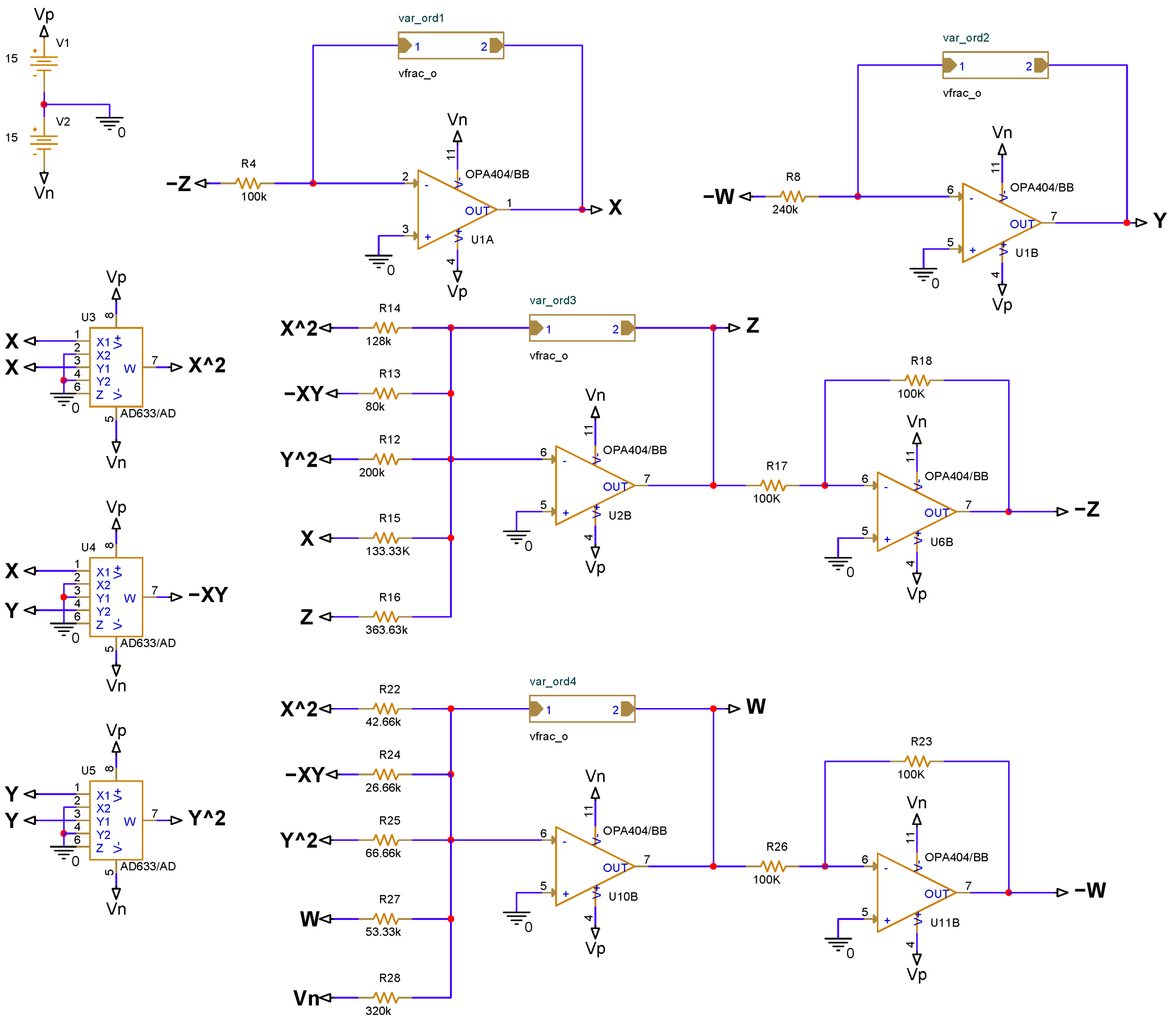
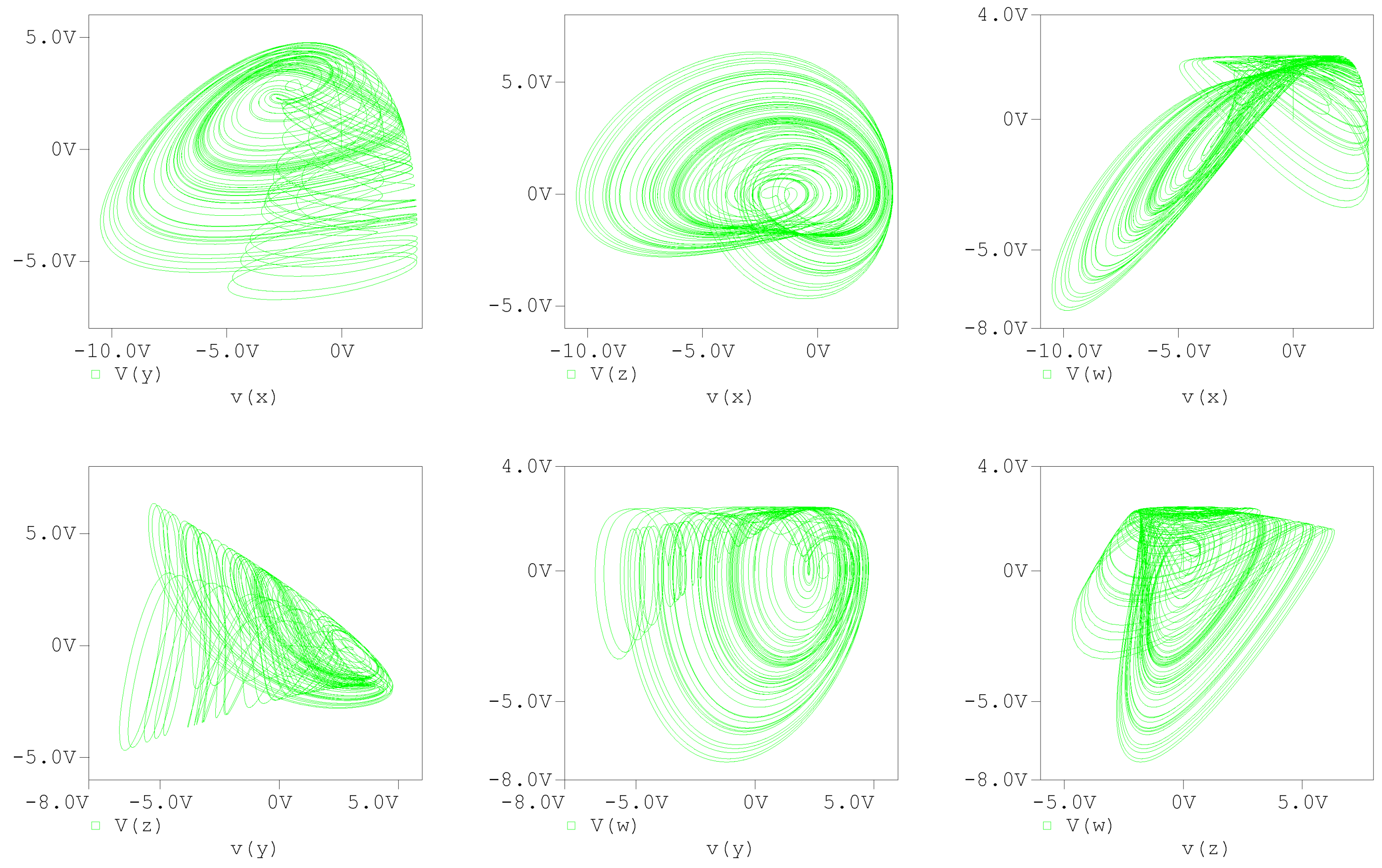
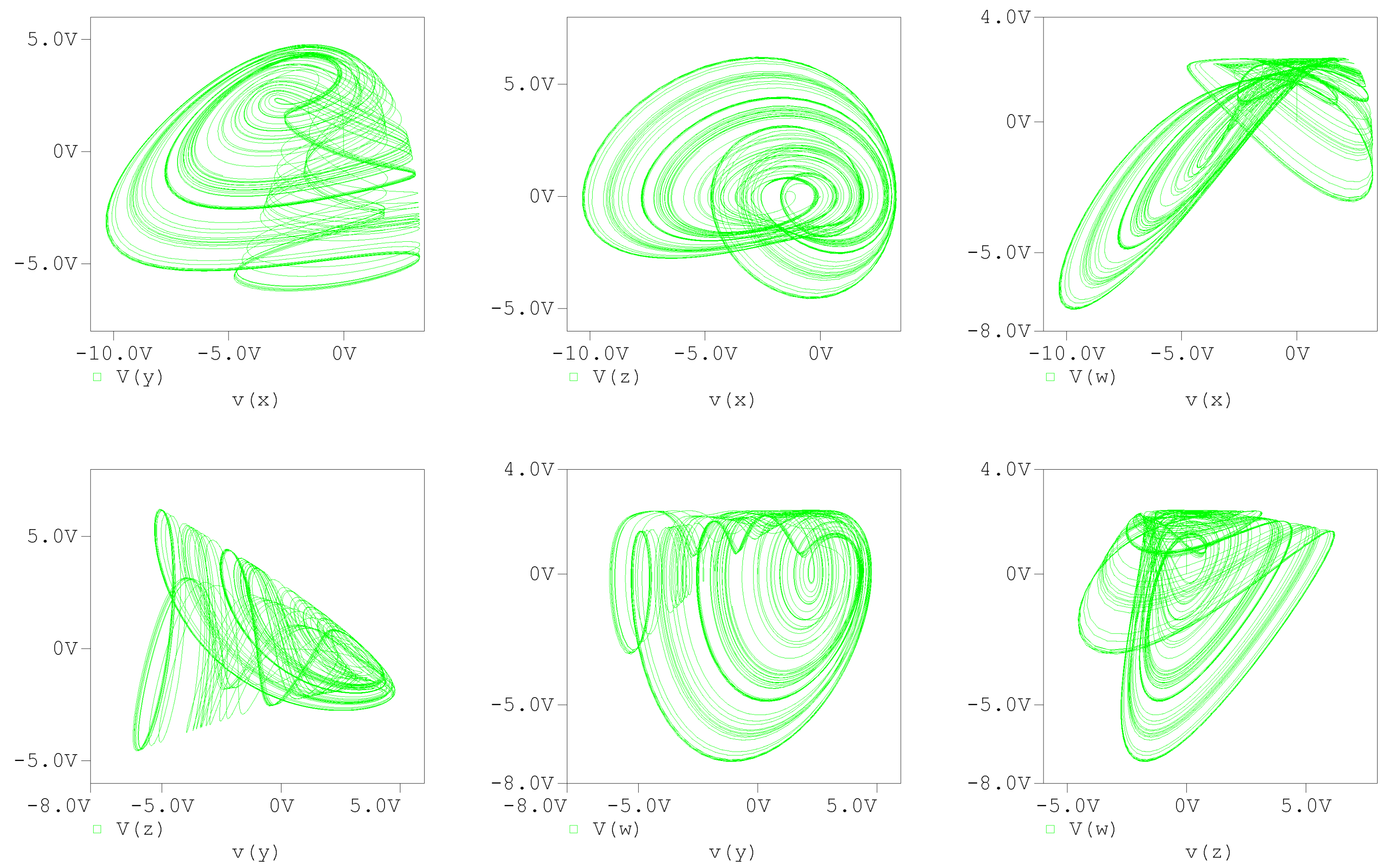
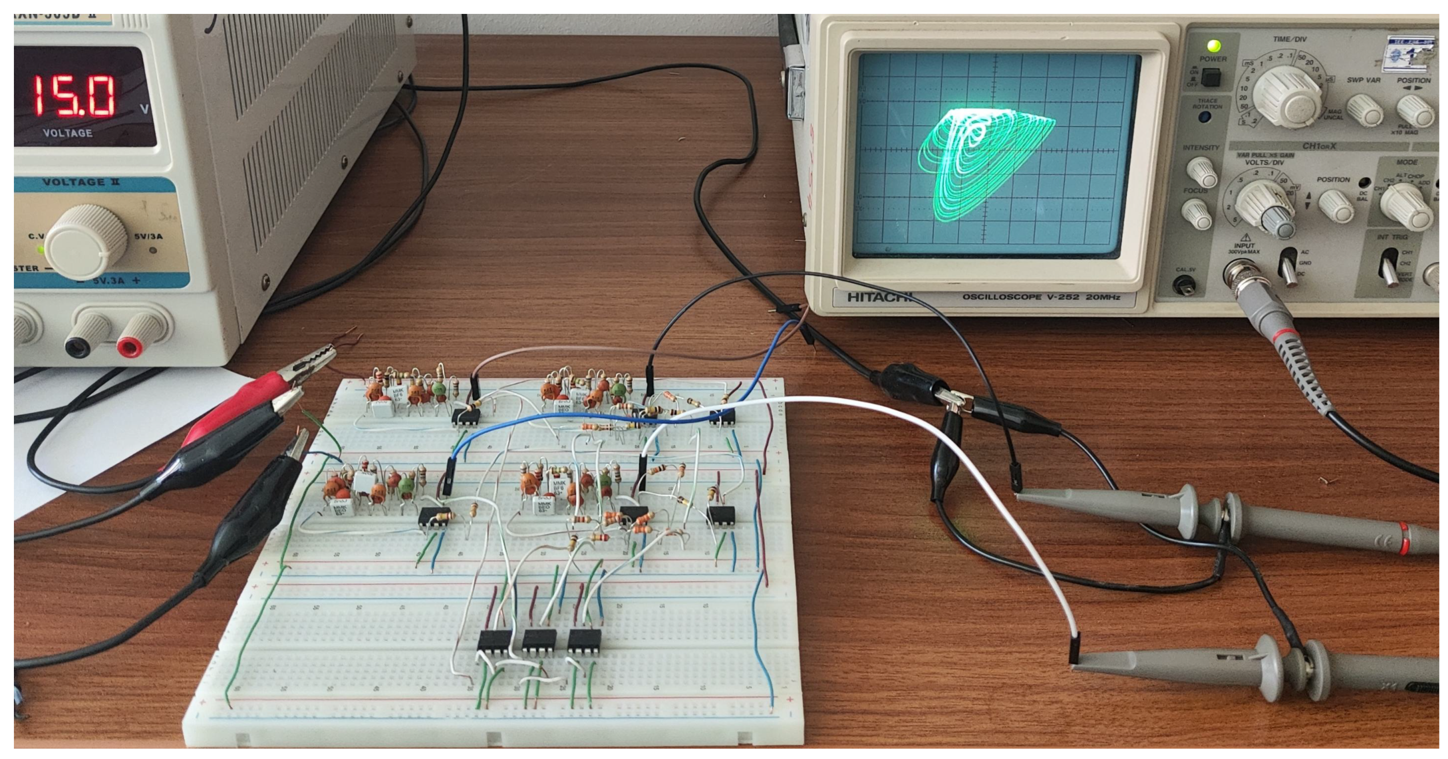
5. Circuit Implementation of Variable Fractional-Order Chaotic System

The computational results are cross-checked with experimental data or theoretical predictions to verify the accuracy and reliability of the simulations. This validation process ensures that the chosen computational model is applicable and capable of accurately predicting real-world behavior [55,56].

In this section, the circuit implementation of the variable fractional-order chaotic system, introduced in the previous section, is given as an example. Here, a variable fractional-order integrator is designed for three different maximum errors y, 0.3 dB, 0.5 dB, and 1 dB, over the frequency range of 0.01 rad/s and 100 rad/s. Bode plots of the approximated transfer functions and the actual transfer function are shown in Figure 7. The circuit implementation of the scaled variable fractional-order chaotic system given in (26) is shown in Figure 8.

Here, as an example, the design process for the first case when the maximum error $y=0.3$ dB is explained in detail.

Since the transfer function of the variable is approximated for the frequency range of 0.01 rad/s and 100 rad/s, the first pole is 0.01.

$$p_0=0.01.$$

(27)

Then, the value of gain k is calculated as

$$k={{10}^{0.3/20}\left.{\displaystyle \frac{\left|\frac{1}{s^{sQ\left(s\right)}}\right|}{1/\left|1+\frac{s}{0.01}\right|}}\right|}_{s=0.01j}\cong 49.55.$$

(28)

Then, the value of zeros and poles are calculated by finding the zero crossings of the plots given in (19) until $p_N$ is greater than or equal to the last frequency of the range ($p_n\ge 100$). The calculated values of poles and zeros are given in

Table 1. The values of poles and zeros when the maximum error $y=0.3$.

n	0	1	2	3	4	5	6	7	8
$p_i$	0.010	0.029	0.039	0.050	0.066	0.094	3.908	78.446	1345.376
$z_i$	0.025	0.033	0.044	0.060	0.086	3.642	73.082	1253.360	-

. When the maximum error $y=0.3$ dB, the number of poles is found as nine, as seen in Table 1.

As an illustrative example of how to determine pole–zero values graphically, the left-hand side of the first four equations in (19) are plotted as functions of the angular frequency $\omega$, where the complex frequency variable s is substituted with $j\omega$. The plots are given in Figure 9.

As shown in Figure 9, the identified pole–zero values are $z_0=0.0252$, $p_1=0.0292$, $z_1=0.0331$, and $p_2=0.0385$. This serves as an illustrative example of how pole–zero values can be determined graphically. However, when dealing with a large number of poles and zeros, manually identifying these values becomes increasingly tedious and error-prone. To address this, Algorithm 1 provides a more practical approach for calculating pole–zero values. The algorithm operates by iteratively detecting the zero crossings of the plotted equations within a while loop structure. At each iteration, the frequency variable is adjusted incrementally until a sign change is observed, indicating the presence of a pole or zero. The pole–zero values, given in Table 1, are obtained using this algorithm.

Since there are nine poles in the approximated transfer function, there will be nine RC tank circuits connected in series as the feedback impedance in the integrator circuit.

After the pole–zero values and the gain k value are calculated, the approximated transfer function is constructed as in (17). Then, partial fraction expansion is performed on the obtained transfer function, and the value of resistors and capacitors is calculated by using (23) and (24). The value of the resistors and capacitors is given in

Table 2. The value of capacitors and resistors in the feedback impedance for the integrator circuit.

n	0	1	2	3	4	5	6	7	8
$C_i$ (F)	2.30	21.87	12.02	7.89	6.28	6.57	13.57	12.67	11.74
$R_i$ ($\Omega$)	43.46	1.56	2.15	2.51	2.40	1.63	0.02	0.001	0.0001

. These values are normalized, with the input-side resistance $R=1\Omega$.

The values of most of the resistors in Table 2 are not practical. This issue can be addressed through the magnitude scaling process. In magnitude scaling, all impedances are multiplied by the same scaling factor. Let $k_m=4\times {10}^5$ be the scaling factor. Then, all impedances in the network will be multiplied by this factor. In other words, the values of resistors are multiplied by $k_m$ while the values of capacitors are multiplied by $1/k_m$, as shown in (29). Here, the value of $R=1\Omega$ in the input side must be multiplied by $k_m$, too. After the magnitude scaling, the value of $R=400$ k$\Omega$ at the input side of the integrator. The value of capacitors and resistors of the magnitude-scaled circuit is given in

Table 3. The value of capacitors and resistors in the feedback impedance for the magnitude-scaled integrator circuit.

n	0	1	2	3	4	5	6	7	8
$C_i$ ($\mu$F)	5.75	54.68	30.06	19.73	15.71	16.41	33.92	31.68	29.36
$R_i$ (k$\Omega$)	17,385.20	623.47	860.50	1004.83	960.70	651.44	7.55	0.60	0.03

.

$$\begin{array}{cc}\hfill & R_i=k_m{R}_i,\hfill \\ \hfill & C_i={\displaystyle \frac{1}{k_m}}{C}_i.\hfill \end{array}$$

(29)

Finally, frequency scaling may be applied depending on the application. In frequency scaling, the frequency is multiplied by a scaling factor while the impedance of the network remains unchanged. Thus, the values of capacitors are multiplied by the inverse of the frequency scaling factor, as shown in (30), while the values of the resistors remain the same. For the frequency scaling process, the scaling factor is selected as $k_f=2500$.

$$C_i={\displaystyle \frac{1}{k_f}}{C}_i.$$

(30)

After the frequency scaling process, the final value of capacitors and resistors is given in

Table 4. The value of capacitors and resistors in the feedback impedance for the frequency- and magnitude-scaled integrator circuit.

n	0	1	2	3	4	5	6	7	8
$C_i$ (nF)	2.30	21.87	12.02	7.89	6.28	6.57	13.57	12.67	11.74
$R_i$ (k$\Omega$)	17,385.20	623.47	860.50	1004.83	960.70	651.44	7.55	0.60	0.03

.

The same procedure is performed for the other cases where the maximum error y equals 0.5 dB and 1 dB, and the values of capacitors and resistors are provided in

Table 5. The value of capacitors and resistors in the feedback impedance for different maximum errors y after magnitude and frequency scaling are performed.

	n	0	1	2	3	4	5
$y=0.5$ dB	$C_i$ (nF)	2.21	9.01	4.61	4.23	7.85	6.97
	$R_i$ (k$\Omega$)	18,089.12	1253.39	15,871.7	1062.10	2.42	0.02
$y=1$ dB	$C_i$ (nF)	1.98	2.41	4.06	3.22	-	-
	$R_i$ (k$\Omega$)	20,179.28	3093.95	24.80	0.002	-	-

.

As seen in Table 5, the approximated transfer function has six and four poles when the maximum error y equals 0.5 and 1 dB, respectively.

All simulations are performed in ORCAD-PSPICE for the calculated values given in Table 4 and Table 5. In all simulations, the initial conditions are set to $X_0=Y_0=Z_0=W_0=0$. For the numerical analysis, the time series are computed over a duration of 200 s. Since the circuit simulations correspond to the frequency-scaled implementation, the simulation time is adjusted accordingly to 80 milliseconds, which is obtained by dividing the numerical run time (200 s) by the frequency scaling factor $k_f=2500$. The phase portraits obtained from simulation results are given in Figure 10, Figure 11 and Figure 12 for a maximum error y equal to 0.3 dB, 0.5 dB, and 1 dB, respectively. As seen in the figures, the lower maximum error y corresponds to more similar phase portraits to ones obtained from the numerical calculations.

For the state variable Y of the system defined in (26), the time series obtained from both numerical calculations and circuit simulations are presented in Figure 13, along with the corresponding error for various values of the maximum approximation error y. Here, y denotes the maximum deviation between the actual and approximated transfer functions of the variable-order integrator. In the simulation setup, the designed integrator circuits are driven by the numerically computed input signal $(25/15)W$, corresponding to the right-hand side of the differential equation governing Y. As shown in Figure 13, the simulation results closely match the numerical calculations when $y=0.3$ dB and $y=0.5$ dB, demonstrating the accuracy and effectiveness of the proposed design method under low-error conditions.

Additionally, a Monte Carlo simulation is conducted on the designed variable-order integrator. In this simulation, resistor tolerances are set at $\pm 5\%$, while capacitor tolerances are set at $\pm 2\%$, with a Gaussian distribution applied to the tolerances. The number of runs for the Monte Carlo simulation is set as 1000. The results show that the maximum absolute error is $0.761$ dB, while the average absolute error is $0.223$ dB for the transfer function of the variable-order integrator circuit.

In the circuit realization, the case in which the maximum error $y=0.5$ dB is selected, since for this case the phase portraits are close to the ones obtained numerically and its Bode plot is close enough to the actual Bode plot. Additionally, the transfer function for this case has three fewer poles than the one for the $y=0.3$ dB case.

The circuit realization and its oscilloscope images are given in Figure 14. As seen in Figure 6, Figure 11 and Figure 14, the phase portraits obtained from numerical calculation, simulation, and circuit realizations are in good accordance.This demonstrates the success of the circuit realization for a time-varying fractional-order chaotic system.

6. Discussion

In this study, a method for the circuit realization of a variable-order chaotic system is proposed. To the best knowledge of the author, this is the first time a circuit for a variable fractional-order chaotic system has been realized in this manner. The method is based on an approximation of the transfer function of the variable fractional-order integrator. Since the transfer function is to be approximated, the variable fractional-order integral definition must be linear time-invariant. There are several definitions of the variable fractional-order integral, but not all are time-invariant. Only the third definition given in [23] is time-invariant. This definition is selected, and numerical calculation results based on the Grünwald–Letnikov method are presented in this paper.

Existing pole–zero calculation methods used for approximating constant fractional-order systems are not applicable to the time-varying fractional-order case due to the dynamic nature of the order function. The key contribution of this work lies in the development of a tailored transfer function approximation framework specifically designed for variable fractional-order integrators. This approach enables the analog realization of such systems through circuit-level synthesis using op-amps and standard passive components.

An example application is conducted in which the time-varying order contains an exponential decaying function and a constant term. The limitations of the proposed method are as follows: The time-varying fractional-order function must be Laplace-transformable, and the Laplace transform must not have any singularities in the frequency range of interest. Furthermore, the slope of the corresponding Bode plot must remain within the range of $-20$ dB/decade and 0 dB/decade.

To validate the proposed method, simulations and circuit realization of the variable fractional-order chaotic system are performed. The phase portraits obtained from numerical calculation, simulation, and circuit realization are in close agreement. This confirms that the proposed method can be used for the circuit realization of the variable-order chaotic system, provided the aforementioned criteria are satisfied.

As a final remark, there is no way of determining the maximum value of y other than trial and error for the results obtained from the realized circuit to be acceptable. For different chaotic systems or/and variable fractional orders, different maximum values of y may produce acceptable results.

Future work will focus on extending the proposed method to cases where the slope of the Bode plot for the time-varying fractional order falls outside the current limitation range.

References

1. Sun, Y.; Cao, L.; Zhang, W. Double color image visual encryption based on digital chaos and compressed sensing. Int. J. Bifurc. Chaos 2023, 33, 2350044. [Google Scholar] [CrossRef]
2. Zhang, B.; Liu, L. Chaos-based image encryption: Review; application; and challenges. Mathematics 2023, 11, 2585. [Google Scholar] [CrossRef]
3. Ming, H.; Hu, H.; Lv, F.; Yu, R. A high-performance hybrid random number generator based on a nondegenerate coupled chaos and its practical implementation. Nonlinear Dyn. 2023, 111, 847–869. [Google Scholar] [CrossRef]
4. Alloun, Y.; Azzaz, M.S.; Kifouche, A. A new approach based on artificial neural networks and chaos for designing deterministic random number generator and its application in image encryption. Multimed. Tools Appl. 2025, 84, 5825–5860. [Google Scholar] [CrossRef]
5. Wang, P.; Zhang, Y.; Yang, H. Research on economic optimization of microgrid cluster based on chaos sparrow search algorithm. Comput. Intell. Neurosci. 2021, 2021, 5556780. [Google Scholar] [CrossRef]
6. Zhang, Y.; Lu, J.; Zhao, C.; Li, Z.; Yan, J. Chaos Optimization Algorithms: A Survey. Int. J. Bifurc. Chaos 2024, 2450205. [Google Scholar] [CrossRef]
7. Silahtar, O.; Kutlu, F.; Atan, Ö.; Castillo, O. Rendezvous and docking control of satellites using chaos synchronization method with intuitionistic fuzzy sliding mode control. In Fuzzy Logic and Neural Networks for Hybrid Intelligent System Design; Springer International Publishing: Cham, Switzerland, 2023; pp. 177–197. [Google Scholar]
8. Kuz’menko, A.A. Forced sliding mode control for chaotic systems synchronization. Nonlinear Dyn. 2022, 109, 1763–1775. [Google Scholar] [CrossRef]
9. Yu, F.; Qian, S.; Chen, X.; Huang, Y.; Liu, L.; Shi, C.; Cai, S.; Song, Y.; Wang, C. A new 4D four-wing memristive hyperchaotic system: Dynamical analysis; electronic circuit design; shape synchronization and secure communication. Int. J. Bifurc. Chaos 2020, 30, 2050147. [Google Scholar] [CrossRef]
10. Bai, C.; Yao, J.L.; Sun, Y.Z.; Ren, H.P. Chaos Division Multi-Access Communication System. IEEE Trans. Circuits Syst. I Regul. Pap. 2024, 71, 5814–5827. [Google Scholar] [CrossRef]
11. Kyriazis, M. Applications of chaos theory to the molecular biology of aging. Exp. Gerontol. 1991, 26, 569–572. [Google Scholar] [CrossRef]
12. Heltberg, M.L.; Krishna, S.; Kadanoff, L.P.; Jensen, M.H. A tale of two rhythms: Locked clocks and chaos in biology. Cell Sys. 2021, 12, 291–303. [Google Scholar] [CrossRef]
13. Chu, Y.M.; Bekiros, S.; Zambrano-Serrano, E.; Orozco-López, O.; Lahmiri, S.; Jahanshahi, H.; Aly, A.A. Artificial macro-economics: A chaotic discrete-time fractional-order laboratory model. Chaos Solitons Fractals 2021, 145, 110776. [Google Scholar] [CrossRef]
14. Fernández-Díaz, A. Overview and perspectives of chaos theory and its applications in economics. Mathematics 2023, 12, 92. [Google Scholar] [CrossRef]
15. Lorenz, E.N. Deterministic nonperiodic flow. J. Atmos. Sci. 1963, 20, 130–141. [Google Scholar] [CrossRef]
16. Iskakova, K.; Alam, M.M.; Ahmad, S.; Saifullah, S.; Akgül, A.; Yılmaz, G. Dynamical study of a novel 4D hyperchaotic system: An integer and fractional order analysis. Math. Comput. Simul. 2023, 208, 219–245. [Google Scholar] [CrossRef]
17. Sun, H.; Zhang, Y.; Baleanu, D.; Chen, W.; Chen, Y. A new collection of real world applications of fractional calculus in science and engineering. Commun. Nonlinear Sci. Numer. Simul. 2018, 64, 213–231. [Google Scholar] [CrossRef]
18. Joshi, M.; Bhosale, S.; Vyawahare, V.A. A survey of fractional calculus applications in artificial neural networks. Artif. Intell. Rev. 2023, 56, 13897–13950. [Google Scholar] [CrossRef]
19. Ionescu, C.; Lopes, A.; Copot, D.; Machado, J.T.; Bates, J.H. The role of fractional calculus in modeling biological phenomena: A review. Commun. Nonlinear Sci. Numer. Simul. 2017, 51, 141–159. [Google Scholar] [CrossRef]
20. Ahmad, S.; Ullah, A.; Akgül, A.; Abdeljawad, T. Chaotic behavior of Bhalekar–Gejji dynamical system under Atangana–Baleanu fractal fractional operator. Fractals 2022, 30, 2240005. [Google Scholar] [CrossRef]
21. Xu, C.; Farman, M.; Shehzad, A. Analysis and chaotic behavior of a fish farming model with singular and non-singular kernel. Int. J. Biomath. 2025, 18, 2350105. [Google Scholar] [CrossRef]
22. Xua, C.; Liaob, M.; Farman, M.; Shehzade, A. Hydrogenolysis of glycerol by heterogeneous catalysis: A fractional order kinetic model with analysis. MATCH Commun. Math. Comput. Chem. 2024, 91, 635–664. [Google Scholar] [CrossRef]
23. Lorenzo, C.F.; Hartley, T.T. Variable order and distributed order fractional operators. Nonlinear Dyn. 2002, 29, 57–98. [Google Scholar] [CrossRef]
24. Sun, H.; Zhang, Y.; Chen, W.; Reeves, D.M. Use of a variable-index fractional-derivative model to capture transient dispersion in heterogeneous media. J. Contam. Hydrol. 2014, 157, 47–58. [Google Scholar] [CrossRef] [PubMed]
25. Sun, H.; Chang, A.; Zhang, Y.; Chen, W. A review on variable-order fractional differential equations: Mathematical foundations; physical models; numerical methods and applications. Fract. Calc. Appl. Anal. 2019, 22, 27–59. [Google Scholar] [CrossRef]
26. Jahanshahi, H.; Sajjadi, S.S.; Bekiros, S.; Aly, A.A. On the development of variable-order fractional hyperchaotic economic system with a nonlinear model predictive controller. Chaos Solitons Fractals 2021, 144, 110698. [Google Scholar] [CrossRef]
27. Macias, M.; Sierociuk, D.; Malesza, W. Realization of the Fractional Variable-Order Model with Symmetric Property. In Proceedings of the Conference on Non-Integer Order Calculus and Its Applications, Białystok, Poland, 20–21 September 2018; pp. 43–54. [Google Scholar]
28. Malesza, W.; Macias, M.; Sierociuk, D. Analytical solution of fractional variable order differential equations. J. Comput. Appl. Math. 2019, 348, 214–236. [Google Scholar] [CrossRef]
29. Jia, H.Y.; Chen, Z.Q.; Qi, G.Y. Chaotic characteristics analysis and circuit implementation for a fractional-order system. IEEE Trans. Circuits Syst. I Regul. Pap. 2014, 61, 845–853. [Google Scholar] [CrossRef]
30. Vaidyanathan, S.; Sambas, A.; Kacar, S.; Cavusoglu, U. A new finance chaotic system; its electronic circuit realization; passivity based synchronization and an application to voice encryption. Nonlinear Eng. 2019, 8, 193–205. [Google Scholar] [CrossRef]
31. Zhou, C.; Li, Z.; Xie, F. Coexisting attractors; crisis route to chaos in a novel 4D fractional-order system and variable-order circuit implementation. Eur. Phys. J. Plus 2019, 134, 73. [Google Scholar] [CrossRef]
32. Yao, J.; Wang, K.; Huang, P.; Chen, L.; Machado, J.T. Analysis and implementation of fractional-order chaotic system with standard components. J. Adv. Res. 2020, 25, 97–109. [Google Scholar] [CrossRef]
33. Arıcıoğlu, B.; Kaçar, S. Circuit implementation and PRNG applications of time delayed Lorenz System. Chaos Theory Appl. 2022, 4, 4–9. [Google Scholar] [CrossRef]
34. Kaçar, S. Digital circuit implementation and PRNG-based data security application of variable-order fractional Hopfield neural network under electromagnetic radiation using Grünwald-Letnikov method. Eur. Phys. J. Spec. Top. 2022, 231, 1969–1981. [Google Scholar] [CrossRef]
35. Emiroglu, S.; Akgül, A.; Adıyaman, Y.; Gümüş, T.E.; Uyaroglu, Y.; Yalçın, M.A. A new hyperchaotic system from T chaotic system: Dynamical analysis, circuit implementation, control and synchronization. Circuit World 2022, 48, 265–277. [Google Scholar] [CrossRef]
36. Charef, A.; Sun, H.H.; Tsao, Y.Y.; Onaral, B. Fractal system as represented by singularity function. IEEE Trans. Autom. Control 1992, 37, 1465–1470. [Google Scholar] [CrossRef]
37. Scherer, R.; Kalla, S.L.; Tang, Y.; Huang, J. The Grünwald–Letnikov method for fractional differential equations. Comput. Math. Appl. 2011, 62, 902–917. [Google Scholar] [CrossRef]
38. Chen, H.; Holland, F.; Stynes, M. An analysis of the Grünwald–Letnikov scheme for initial-value problems with weakly singular solutions. Appl. Numer. Math. 2019, 139, 52–61. [Google Scholar] [CrossRef]
39. Liouville, J. Mémoire Sur quelques Questions de Géometrie et de Mécanique, et sur un nouveau genre de Calcul pour résoudre ces Questions. J. L’École Polytech. 1832, 13, 1–69. [Google Scholar]
40. Riemann, B. Versuch einer allgemeinen Auffassung der Integration und Differentiation. Gesammelte Werke 1876, 62, 52–61. [Google Scholar]
41. Grünwald, A.K. Uber “begrente” Derivationen und deren Anwedung. Z. Angew. Math. Phys. 1867, 12, 441–480. [Google Scholar]
42. Letnikov, A.V. Theory of differentiation with an arbtraly indicator. Matem Sb. 1868, 3, 1–68. [Google Scholar]
43. Tarasov, V.E. Lattice model of fractional gradient and integral elasticity: Long-range interaction of Grünwald–Letnikov–Riesz type. Mech. Mater. 2014, 70, 106–114. [Google Scholar] [CrossRef]
44. Sierociuk, D.; Malesza, W.; Macias, M. On the recursive fractional variable-order derivative: Equivalent switching strategy, duality, and analog modeling. Circuits Syst. Signal Process. 2015, 34, 1077–1113. [Google Scholar] [CrossRef]
45. Sierociuk, D.; Malesza, W.; Macias, M. Derivation, interpretation, and analog modelling of fractional variable order derivative definition. Appl. Math. Model. 2015, 39, 3876–3888. [Google Scholar] [CrossRef]
46. Ahmad, W.M.; Sprott, J.C. Chaos in fractional-order autonomous nonlinear systems. Chaos Solitons Fractals 2003, 16, 339–351. [Google Scholar] [CrossRef]
47. Kacar, S.; Wei, Z.; Akgul, A.; Aricioglu, B. A novel 4D chaotic system based on two degrees of freedom nonlinear mechanical system. Z. Naturforschung A 2018, 73, 595–607. [Google Scholar] [CrossRef]
48. Moysis, L. Bifurcation Diagram for the Lorenz System (Local Maxima). 2025. Available online: https://www.mathworks.com/matlabcentral/fileexchange/158081-bifurcation-diagram-for-the-lorenz-system-local-maxima (accessed on 11 April 2025).
49. Li, H.; Shen, Y.; Han, Y.; Dong, J.; Li, J. Determining Lyapunov exponents of fractional-order systems: A general method based on memory principle. Chaos Solitons Fractals 2023, 168, 113167. [Google Scholar] [CrossRef]
50. Gottwald, G.A.; Melbourne, I. A new test for chaos in deterministic systems. Proc. R. Soc. Lond. Ser. A Math. Phys. Eng. Sci. 2004, 460, 603–611. [Google Scholar] [CrossRef]
51. Cui, Q.; Xu, C.; Xu, Y.; Ou, W.; Pang, Y.; Liu, Z.; Shen, J.; Baber, M.Z.; Maharajan, C.; Ghosh, U. Bifurcation and Controller Design of 5D BAM Neural Networks with Time Delay. Int. J. Numer. Model. Electron. Netw. Devices Fields 2024, 37, e3316. [Google Scholar] [CrossRef]
52. Zhao, Y.; Xu, C.; Xu, Y.; Lin, J.; Pang, Y.; Liu, Z.; Shen, J. Mathematical exploration on control of bifurcation for a 3D predator-prey model with delay. AIMS Math. 2024, 9, 29883–29915. [Google Scholar] [CrossRef]
53. Berkal, M.; Almatrafi, M.B. Bifurcation and stability of two-dimensional activator–inhibitor model with fractional-order derivative. Fractal Fract. 2023, 7, 344. [Google Scholar] [CrossRef]
54. Berkal, M.; Navarro, J.F.; Hamada, M.Y.; Semmar, B. Qualitative behavior for a discretized conformable fractional-order predator–prey model. J. Appl. Math. Comput. 2025, 1–23. [Google Scholar] [CrossRef]
55. Bhatti, M.M.; Marin, M.; Ellahi, R.; Fudulu, I.M. Insight into the dynamics of EMHD hybrid nanofluid (ZnO/CuO-SA) flow through a pipe for geothermal energy applications. J. Therm. Anal. Calorim. 2023, 148, 14261–14273. [Google Scholar] [CrossRef]
56. Yadav, A.K.; Carrera, E.; Marin, M.; Othman, M.I.A. Reflection of hygrothermal waves in a Nonlocal Theory of coupled thermo-elasticity. Mech. Adv. Mater. Struct. 2024, 31, 1083–1096. [Google Scholar] [CrossRef]
Figure 1. The Bode plot of a variable fractional-order integrator and its approximation with zig-zag lines.
Axioms 14 00310 g001
Figure 2. An inverting fractional-order integrator circuit.
Axioms 14 00310 g002
Figure 3. The Lyapunov exponents of the variable-order chaotic system.
Axioms 14 00310 g003
Figure 4. The Lyapunov exponents of the variable fractional-order chaotic system with respect to the parameters’ values when the fractional order q ( t ) = 0.76 + 0.215 e 0.05 t and the initial conditions are x 0 = y 0 = z 0 = w 0 = 0 .
Axioms 14 00310 g004
Figure 5. Bifurcation diagram with respect to q.
Axioms 14 00310 g005
Figure 6. The phase portraits of the scaled variable fractional-order chaotic system for the fractional order q ( t ) = 0.76 + 0.215 e 0.05 t ; the system parameters are α = 1.1 , β = 12 , ρ = 25 , γ = 1.25 , σ = 7.5 , and ζ = 25 , and the initial conditions are x 0 = y 0 = z 0 = w 0 = 0 .
Axioms 14 00310 g006
Figure 7. The Bode plots of actual and approximated transfer functions for (a) y = 0.3 dB, (b) y = 0.5 dB, and (c) y = 1 dB (the red line is the actual transfer function; the blue line is the approximated transfer function).
Axioms 14 00310 g007
Figure 8. The circuit implementation of the variable fractional-order chaotic system.
Axioms 14 00310 g008
Figure 9. Determining the pole–zero values graphically.
Axioms 14 00310 g009
Figure 10. The phase portraits obtained from the simulation when the maximum error y = 0.3 dB.
Axioms 14 00310 g010
Figure 11. The phase portraits obtained from the simulation when the maximum error y = 0.5 dB.
Axioms 14 00310 g011
Figure 12. The phase portraits obtained from the simulation when the maximum error y = 1 dB.
Axioms 14 00310 g012
Figure 13. The numerical calculation and simulation results for the time series of Y state variable of (26) for (a) y = 0.3 dB, (b) y = 0.5 dB, and (c) y = 1 dB.
Axioms 14 00310 g013
Figure 14. The circuit realization of the variable fractional-order chaotic system and the phase portraits obtained from the circuit realization when the maximum error y = 0.5 dB.
Axioms 14 00310 g014aAxioms 14 00310 g014b