Abstract
In this paper, we outline a method for constructing nonnegative scaling vectors on the interval. Scaling vectors for the interval have been constructed in [1,2,3]. The approach here is different in that the we start with an existing scaling vector Φ that generates a multi-resolution analysis for to create a scaling vector for the interval. If desired, the scaling vector can be constructed so that its components are nonnegative. Our construction uses ideas from [4,5] and we give results for scaling vectors satisfying certain support and continuity properties. These results also show that less edge functions are required to build multi-resolution analyses for than the methods described in [5,6].
1. Introduction
Let ϕ be a compactly supported orthogonal scaling function generating a multi-resolution analysis, , for . In Walter and Shen [7], the authors show how to use this ϕ to construct a new nonnegative scaling function P that generates the same multi-resolution analysis for . The disadvantages of this construction is that orthogonality is lost (although the authors gave a simple expression for the dual ), and P is not compactly supported.
The results of [7] were generalized to the scaling vectors in [8]. In [9], the authors show that it is possible to modify the construction of [8] and retain compact support. Since many applications require the underlying space to be , rather than , it is worthwhile to investigate extending the construction to the interval.
In this paper, we take a continuous, compactly supported scaling vector Φ and illustrate how it can be used to construct a compactly supported scaling vector P that generates a multi-resolution analysis for . The resulting scaling vector for is nonnegative if at least one component of the original scaling vector Φ is nonnegative on its support. Nonnegativity of the scaling vector may be desirable in applications, such as density estimation (see [10] for density estimation by a single nonnegative scaling function). The construction is motivated by the work of Meyer [5]. It is a goal of the construction to produce a nonnegative scaling vector, preserve the polynomial accuracy of the original scaling vector and to keep the number of edge functions as small as possible. We conclude the paper with results that show, under certain circumstances, that it is possible to construct compactly scaling vectors that require only edge functions to preserve polynomial accuracy m. This is an improvement over some methods (for example, [5,6]) that require m edge functions to preserve polynomial accuracy m.
In the next section, we introduce basic definitions, examples and results that are used throughout the sequel. In the third section, we define the edge functions for our constructions and show that the resulting scaling vector satisfies a matrix refinement equation and generates a multi-resolution analysis for . The final section consists of some constructions illustrating the results of Section 3, as well as results in special cases that show the number of edge functions needed to attain a desired polynomial accuracy is smaller than the number needed for similar methods.
2. Notation, Definitions and Preliminary Results
We begin with the concept of a scaling vector or set of multiscaling functions. This idea was first introduced in [11,12]. We start with A functions, , and consider the nested ladder of subspaces, , where , .
It is convenient to store as a vector:
and define a multi-resolution analysis in much the same manner as in [4]:
- (M1)
- .
- (M2)
- .
- (M3)
- , .
- (M4)
- , .
- (M5)
- Φ generates a Reisz basis for .
In this case, Φ satisfies a matrix refinement equation:
We will make the following two assumptions about Φ and its components:
- (A1)
- Each , , is compactly supported and continuous;
- (A2)
- There is a vector for which:
Condition (A2) tells us that Φ forms a partition of unity.
We will say that Φ has polynomial accuracy m if there exist constants such that for
where
We have the following result from [13] involving the components of the vectors :
Lemma 2.1 ([13]). The components of the vectors in Equations (4) satisfy the recurrence relation
for , and .
It will be convenient to reformulate Equation (5) in the following way:
Proposition 2.2. For the row vectors given in Equation (4), define the column vectors
Then
where is the lower triangular Pascal matrix, whose elements are defined by
for .
The following corollary is immediate:
Corollary 2.3. For , we have:
Note: We have defined the vectors without including the term . While Proposition 2.2 certainly holds if this term is included in the definition of , our results in Section 4 use as defined by Equation (6).
With regards to (A1), we will further assume that for , ,
We will denote by M the maximum value of :
As stated in Section 1, our construction of scaling vector for uses an existing scaling vector Φ for . It is possible to perform our construction, so that the components of are nonnegative. If the components of Φ are nonnegative, then the components of will be nonnegative, as well. In the case where not all the components of Φ are nonnegative, it still may be possible to construct a nonnegative . Theorem 2.5 from [9] illustrates that in order to do so, we must first modify Φ. To this end, Φ must be bounded and compactly supported, possess polynomial accuracy, , and satisfy Condition B below.
Definition 2.4 (Condition B). Let . We say Φ satisfies Condition B if for some , for and there exist finite index sets and constants for , such that:
- (B1)
- , ,
- (B2)
- ,
- (B3)
- for
Here, the are the coefficients from (A2).
Theorem 2.5 ([9]). Suppose a scaling vector , is bounded, compactly supported, has accuracy, , and satisfies Condition B. Then the nonnegative vector
where is given by (B1) and is a bounded, compactly supported scaling vector with accuracy that generates the same space, .
We now give two examples of multiscaling functions that we will use in the sequel.
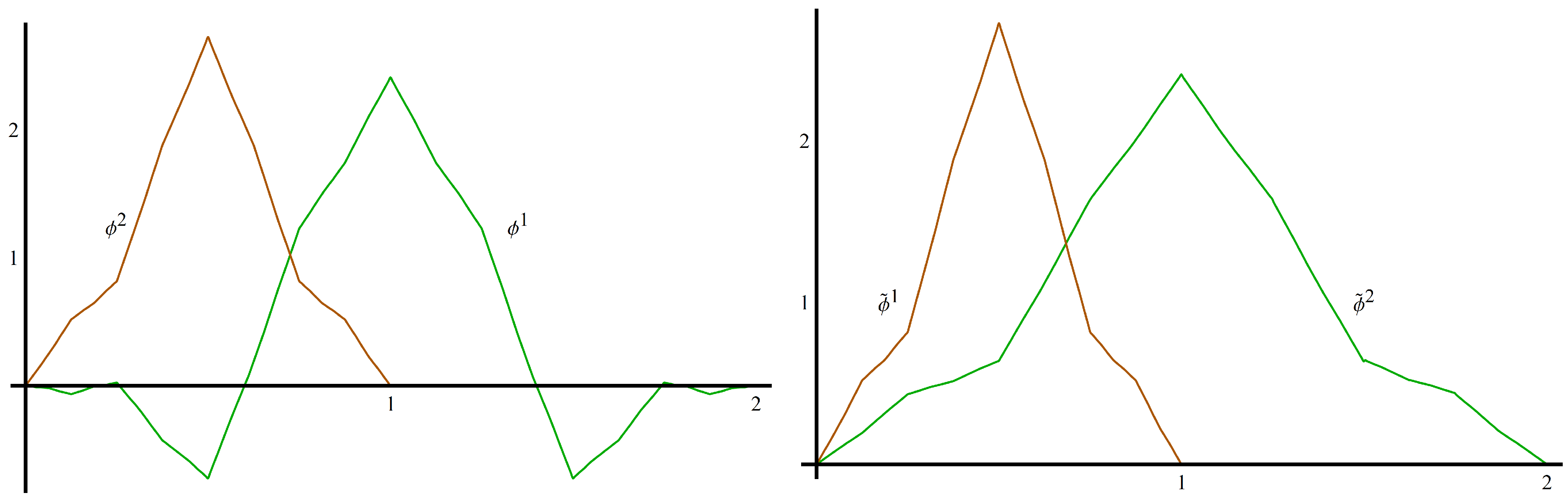
Example 2.6 (Donovan,Geronimo,Hardin,Massopust). In [14], the authors constructed a scaling vector with that satisfies the four-term matrix refinement equation, , where
The scaling functions , (shown in Figure 1), satisfy , , . They also have polynomial accuracy two are continuous, symmetric and compactly supported with and . Φ also satisfies the partition of unity condition (A2) with
We can satisfy Theorem 2.5 by choosing , since , . We create by taking with , so that for . The partition of unity coefficients for are and . The new scaling vector, , is shown in Figure 1.
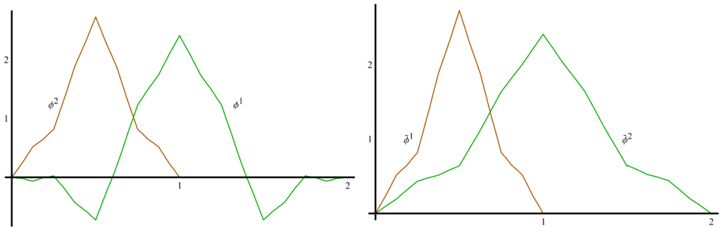
Figure 1.
The scaling vector Φ (left) and the new scaling vector from Example 2.6 (right).
Figure 1.
The scaling vector Φ (left) and the new scaling vector from Example 2.6 (right).
Our next example uses a scaling vector constructed by Plonka and Strela in [15].
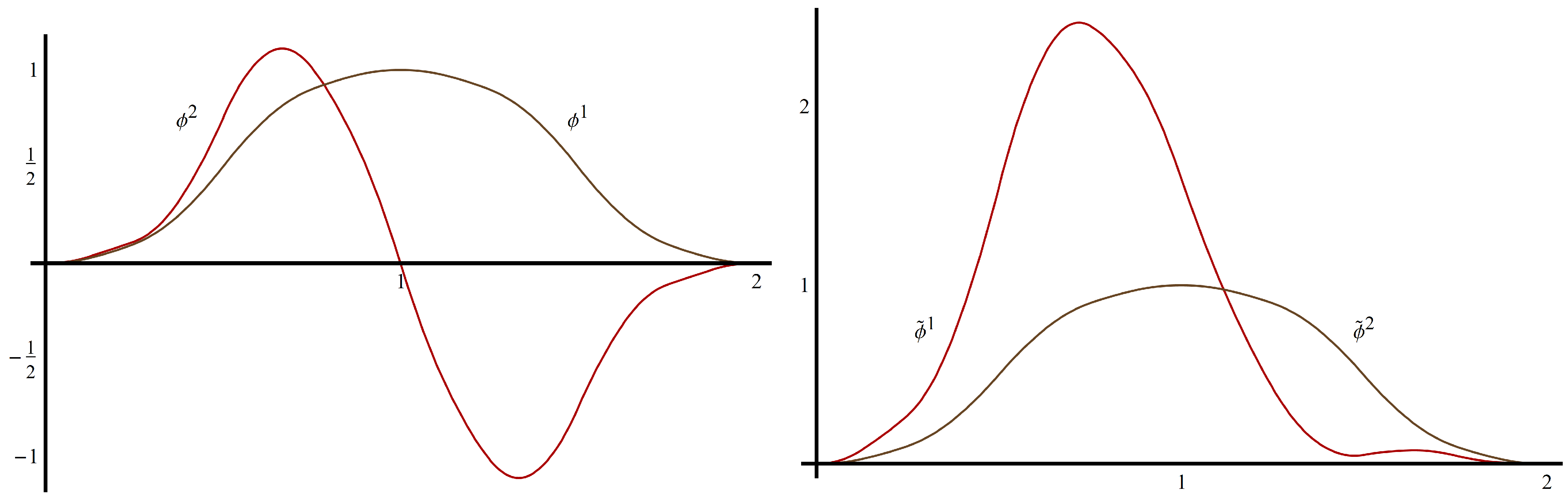
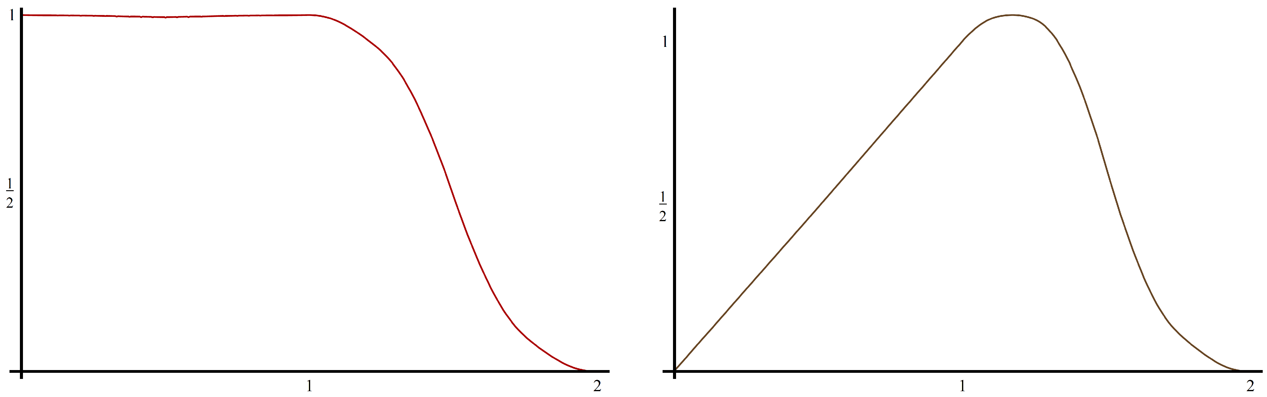
Example 2.7 (Plonka,Strela). Using a two-scale similarity transform in the frequency domain, Plonka and Strela constructed the following scaling vector Φ in [15]. It satisfies a three-term matrix refinement equation
where
This scaling vector (shown in Figure 2) is not orthogonal, but it is compactly supported on with polynomial accuracy three. is nonnegative on its support and symmetric about , while is antisymmetric about . Φ satisfies (A2) with , . The authors also show that
We can satisfy Theorem 2.5 by choosing since , . We create by taking , so that for . The partition of unity coefficients for are and . The new scaling vector is shown in Figure 2.
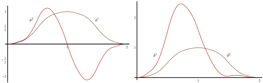
Figure 2.
The scaling vector Φ (left) and the the new scaling vector from Example 2.7 (right).
Figure 2.
The scaling vector Φ (left) and the the new scaling vector from Example 2.7 (right).
3. Nonnegative Scaling Vectors on the Interval
The construction of scaling vectors on the interval has been addressed in [1,2,3]. In these cases, the authors constructed scaling vectors on the interval from scratch. It is our intent to show how to modify a given scaling vector that generates a multi-resolution analysis for , so that it generates a (nonorthogonal) multi-resolution analysis for . Moreover, the components of the new vector will be nonnegative. In particular cases, our procedure requires fewer edge functions than in the single scaling function constructions of [5,6].
Our task then is to modify an existing scaling vector and create a nonnegative scaling vector that generates a multi-resolution analysis for that preserves the polynomial accuracy of the original scaling vector and avoids the creation of “too many” edge functions.
We begin with a multi-resolution analysis for generated by scaling vector Φ and we also assume our scaling vector has polynomial accuracy m with given by Equation (4).
Finally, assume that the set of non-zero functions defined by are linearly independent, and let denote the number of functions in S. Note that, due to the support restriction of Φ in Equation (10), .
Note that S consists of all the original scaling functions , plus those left shifts, , , whose support overlaps . Since each scaling function is supported on , we can compute
We work only on the left edge in constructing . We begin with , and then add left edge functions to preserve polynomial accuracy.
Define the left edge functions, , by
for . Observe that since the are compactly supported, so is and also note that by Equation (3), on . Right edge functions can be defined similarly.
Our next proposition shows that the left edge functions (and, in an analogous manner, the right edge functions) satisfy a matrix refinement equation.
Proposition 3.1. Suppose that Φ is a scaling vector satisfying (A1)–(A2) with polynomial accuracy m with , given in Equation (3). Further assume that the set S defined above is linearly independent. Then the set of edge functions , , satisfies a matrix refinement equation.
Proof. Φ satisfies a matrix refinement Equation (1), and since Φ is supported on , the number of refinement terms is finite. So there is a minimal positive integer N such that
with for or . Now for we have
Note that for each and :
We are able to leave the summation limits on the inner sum in the above line unchanged, since for or . Thus we have
with
Recall that on and that the functions are linearly independent, so for . Thus
on . This is the desired dilation equation for the edge function, . ☐
Refinement equations for the right edge functions are derived in a similar manner.
Example 3.2. We return to the scaling vector of Strela and Plonka [15] introduced in Example 2.7. This scaling vector has polynomial accuracy three with and .
Both and are supported on . The refinement equation matrices, , and , are given in Example 2.7. We calculate and as:
and
The dilation equation for is
In a similar manner, we can use Equations (13) and (16) to find that
We thus compute the dilation equation for :
In order to construct a scaling vector for , we need for our edge functions not only to satisfy a matrix refinement equation, but also to join with and form a Riesz basis for . We will next show that the set of edge functions we constructed above does indeed preserve the Riesz basis property. We need the following result.
Lemma 3.3. Suppose H is a separable Hilbert space with closed subspaces, V,,W and , such that . Assume further that V and are topologically isomorphic with Riesz bases, , , respectively, and W and are topologically isomorphic with Riesz bases, , , respectively. Then, and are topologically isomorphic with Riesz bases, , , respectively.
Proof. First we present a useful fact to simplify the proof. As stated in [4] (page xix), every Riesz basis is a homeomorphic image of an orthonormal basis. Since V and are homeomorphic images of each other, we can assume without loss of generality, that the bases and are orthonormal bases of V and , respectively. Similarly we may assume that the bases and are orthonormal bases of W and , respectively.
Now, to show that is a Riesz basis of , we need to verify the stability condition:
for some and for all sequences, , where, for convenience, we partition as .
Use the orthonormality of the sets and to obtain
so
Now we use Equation (18) to see that
which proves the upper bound on the stability condition of Equation (17) with .
We use Bessel’s inequality with each orthonormal set and to obtain
Adding these inequalities, we find the lower stability bound for Equation (17) with :
This completes the proof that is a Riesz basis of and an identical argument shows that is a Riesz basis of .
It is now easy to see that the map , which maps each to and each to , is a homeomorphism. ☐
We are now ready to state and prove our next result.
Theorem 3.4. Let be a scaling vector that satisfies (A1) and generates a multi-resolution analysis for . For some index set B, let be a finite set of edge functions with and assume that is a linearly independent set. Then is a Riesz basis of , where .
Proof. Without loss of generality, set , and let C be the set of integer indices for which for all . For ease of notation, denote by those corresponding to C, and for integer index set D, let denote the other . For ease of presentation, assume that B,C and D are mutually disjoint and note that . Now, since is a linearly independent and a finite set, it must be a Riesz basis of its span. We then use the Gram-Schmidt process to orthogonalize it and thus obtain . In the process, we begin with the and then move on to the . This ensures that , whence for all .
If we set and , we have , so by Lemma 3.3, has Riesz basis . Hence there exist , such that
Assuming without loss of generality that , we use the line above, , the orthogonality of the and the disjoint support of the and to see that
A similar proof shows that
so is a Riesz basis of its span. Finally, to see that is a Riesz basis for , set and and . Since has finite dimension and , Lemma 3.3 holds so that is a Riesz basis for . ☐
4. Edge Function Construction
We begin this section by constructing the left edge function needed to build the interval scaling vector from the scaling vector of Example 2.6.
Example 4.1. We return to the scaling vector of Example 2.6. Note that and
It is known (see for example [16]) that Φ can be restricted to any interval, , where and the set
constitutes an orthogonal set of functions on and reproduces constant functions on . We nevertheless construct the edge function to illustrate the computation and provide motivation for Theorem 4.2.
We use Equation (15) to construct :
If we want a nonnegative edge function, then we need to use from Example 2.6. In this case
Using Equation (15), we see that
The edge functions are plotted in Figure 3.
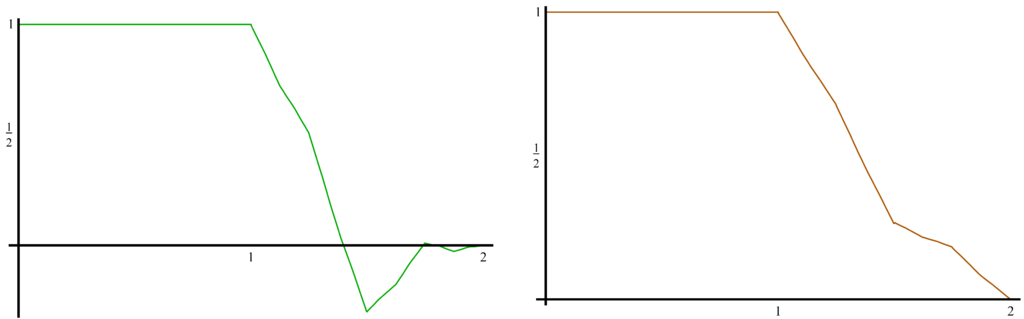
Figure 3.
The edge function using (left) and the nonnegative edge function using (right) from Example 4.1.
Figure 3.
The edge function using (left) and the nonnegative edge function using (right) from Example 4.1.

Although for the scaling vector in Example 4.1, we only computed . There is a good reason for this: it turns out that can be written as a linear combination of Φ and . Indeed, we can use Equation (3) and the supports of and to write
and then ask if there exists constants , , such that
Expanding this system and equating coefficients for , and gives
To motivate further results we write the above system as the matrix equation
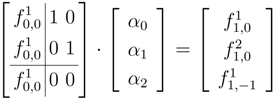 Note that the uniqueness of a solution to this system is completely determined by the fact that .
Thus for the scaling vector of Example 4.1, we need only one left (right) edge function to form a multi-resolution analysis for . This is one fewer left (right) edge functions than required by the constructions of multi-resolution analyses described in [5,6].
The preceding discussion provides motivation for the following result.
Theorem 4.2. Suppose forms a multi-resolution analysis for with polynomial accuracy . Suppose that each is continuous on , , and for . Then for , can be written as a linear combination of , and , . That is, only the left (right) edge functions defined by Equation (15) are needed in conjunction with Φ to construct a multi-resolution analyses of .
Proof. It suffices to show that there exists , such that
for .
From Equation (15) and the support properties of Φ, we know that , can be expressed as
Expanding the right-hand side of Equation (20) gives
Equating coefficients for , , and , , in Equations (21) and (22) gives rise to the following system of linear equations
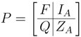
We can reformulate Equation (23) as a matrix equation, , where
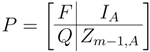 with the identity matrix, the zero matrix, F the matrix defined component-wise by , and Q the matrix given by
The proof is complete if we can show Q is a nonsingular matrix.
with the identity matrix, the zero matrix, F the matrix defined component-wise by , and Q the matrix given by
The proof is complete if we can show Q is a nonsingular matrix.
Using Equation (6) and Corollary 2.3, we see that
where is the lower-triangular Pascal matrix given by Equation (8). Thus
where we have introduced the row vector for ease of notation, and is the upper-triangular Pascal matrix defined by .
We can perform the following row operations on the right-hand side of Equation (25), and the result has the same determinant as Q
An identity given in [17] leads to , where is the diagonal matrix, whose diagonal entries are , , so that
The matrix is strictly upper triangular with zeros in every diagonal until the kth upper diagonal. Denote by the first element in this diagonal, and note that , since every element in the kth diagonal and above in is positive. Pre- and post-multiplication by D only serves to change signs of various elements of . In particular, the first element in the kth upper diagonal of Equation (27) is . Thus the matrix on the right-hand side of Equation (26) is upper triangular with with diagonal elements, , . Hence Q is non-singular if . However is a continuous scaling vector that forms a partition of unity. Since for , the only way to satisfy the partition of unity condition at the nonzero integers is if . ☐
We return to Example 2.7 to motivate our next result.
Example 4.3. The scaling vector Φ from Example 2.7 has polynomial accuracy and . We construct the edge functions and . Noting that and , we have
and
where we have used Lemma 2.1 to compute and . The edge functions are plotted in Figure 4.
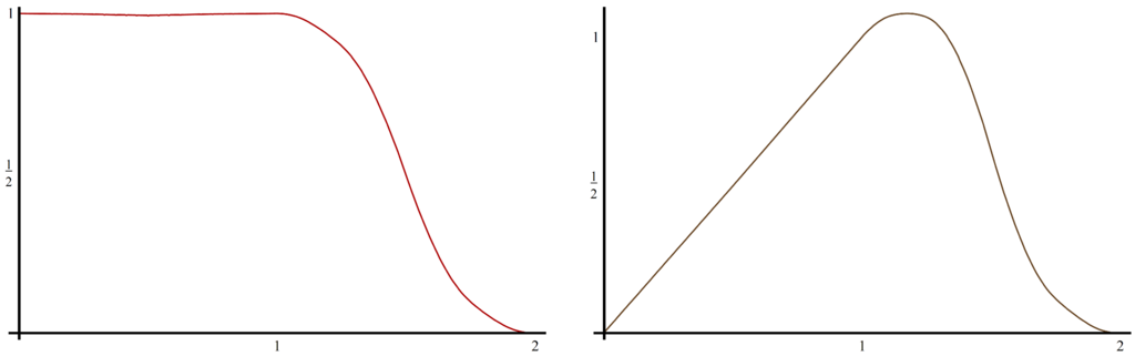
Figure 4.
The edge functions, and , from Example 4.3.
Figure 4.
The edge functions, and , from Example 4.3.
We did not construct because it can be constructed as a linear combination of , , and . We know for . For , we have
We seek , so that
for . We can regroup the terms in Equation (29) as follows:
Comparing this Equation to (28) leads to the following system of equations
This system is easily seen to have a unique solution.
We can generalize the preceding discussion with the following proposition:
Theorem 4.4. Suppose forms a multi-resolution analysis for with polynomial accuracy . Suppose that each is continuous on and , . Assume further that is a linearly independent set of vectors. Then for , can be written as a linear combination of , , and , . That is, only the left (right) edge functions defined by Equation (15) are needed in conjunction with Φ to construct a multi-resolution analyses of .
Proof. We seek constants, , such that for , we have
Substituting the edge functions
into Equation (30) gives, for
However for
Setting Equations (31) and (32) equal to each other gives rise to the following system of equations
We can reformulate Equation (33) as a matrix equation, , where
and
 with and the identity and zero matrices, respectively, F the matrix defined component-wise by and Q the matrix given by
The proof is complete if we can show Q is a nonsingular matrix.
with and the identity and zero matrices, respectively, F the matrix defined component-wise by and Q the matrix given by
The proof is complete if we can show Q is a nonsingular matrix.
Using Equation (6) and Corollary 2.3, we see that
Since it is assumed that is a linearly independent set of vectors, is nonsingular and the proof is complete. ☐
Propositions 4.2 and 4.4 in some sense represent the extreme cases for the supports of scaling functions in Φ. In the general case, , and in order to consider a square system, like Equations (23) or (33), we need the number of functions in contributing to for , which should be the sum of (the number of edge functions) and A (the number of scaling functions). From Equation (14), we have
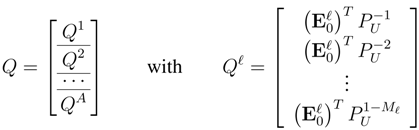
so that . Using an argument similar to those used in the proofs of Propositions 4.2 and 4.4, we would arrive at the system , where
with and
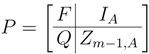 where is the identity matrix, is the zero matrix, F is the matrix defined component-wise by , , and Q is the matrix given in block form by
 for .
for .
It remains an open problem to determine the conditions necessary to ensure Q is nonsingular. A reasonable assumption is that (or equivalently, the set ) is a set of linearly independent vectors, but the proof has not been established. For those instances when , it must be true that , since this vector is an eigenvector of .
It is also unclear whether or not nonnegative scaling vectors can be created that possess certain (anti-)symmetry properties. If the underlying scaling vector possesses (anti-)symmetry properties, then the only modifications needed would be for the edge functions. We have yet to consider the problem of creating (anti-)symmetric edge functions.
Acknowledgments
The authors wish to express their gratitude to University of St. Thomas colleague, Yongzhi (Peter) Yang, for introducing us to several interesting properties obeyed by Pascal matrices and for his careful reading of the manuscript.
References
- Dahmen, W.; Micchelli, C.A. Biorthogonal wavelet expansions. Constr. Approx. 1997, 13, 293–328. [Google Scholar] [CrossRef]
- Goh, S.; Jian, Q.; Xia, T. Construction of biorthogonal multiwavelets using the lifting scheme. Appl. Comput. Harm. Anal. 2000, 9, 336–352. [Google Scholar] [CrossRef]
- Lakey, J.; Pereyra, C. Divergence-Free Multiwavelets on Rectangular Domains. In Wavelet Analysis and Multiresolution Methods; Marcel Dekker: Urbana-Champaign, IL, USA, 2000; pp. 203–240. [Google Scholar]
- Daubechies, I. Ten Lectures on Wavelets; SIAM: Philadelphia, PA, USA, 1992. [Google Scholar]
- Meyer, Y. Ondelettes sur l‘intervalle. Rev. Math. Iberoam. 1991, 7, 115–133. [Google Scholar] [CrossRef]
- Cohen, A.; Daubechies, I.; Vial, P. Wavelets on the interval and fast wavelet transforms. Appl. Comput. Harmon. Anal. 1993, 1, 54–81. [Google Scholar] [CrossRef]
- Walter, G.; Shen, X. Positive estimation with wavelets. Cont. Math. 1998, 216, 63–79. [Google Scholar]
- Ruch, D.; Van Fleet, P. On the Construction of Positive Scaling Vectors. In Proceedings of Wavelet Analysis and Multiresolution Methods, New York, USA, 2000; He, T., Ed.; Marcel Dekker: New York, NY, USA, May 2000; pp. 317–339. [Google Scholar]
- Ruch, D.; Van Fleet, P. Gibbs’ phenomenon for nonnegative compactly supported scaling vectors. J. Math. Anal. Appl. 2005, 5, 370–382. [Google Scholar] [CrossRef]
- Walter, G.; Shen, X. Continuous nonnegative wavelets and their use in density estimation. Commut. Stat. Theory Method 1999, 28, 1–18. [Google Scholar] [CrossRef]
- Geronimo, J.; Hardin, D.; Massopust, P. Fractal functions and wavelet expansions based on several scaling functions. J. Approx. Theory 1994, 78, 373–401. [Google Scholar] [CrossRef]
- Goodman, T.; Lee, S.L. Wavelets of multiplicity r. Trans. Am. Math. Soc. 1994, 342, 307–324. [Google Scholar]
- Heil, C.; Strang, G.; Strela, V. Approximation by translates of refinable functions. Numer. Math. 1996, 73, 75–94. [Google Scholar] [CrossRef]
- Donovan, G.; Geronimo, J.; Hardin, D.; Massopust, P. Construction of orthogonal wavelets using fractal interpolation functions. SIAM J. Math. Anal. 1996, 27, 1158–1192. [Google Scholar] [CrossRef]
- Plonka, G.; Strela, V. Construction of multiscaling functions with approximation and symmetry. SIAM J. Math. Anal. 1998, 29, 481–510. [Google Scholar] [CrossRef]
- Donovan, G.; Geronimo, J.; Hardin, D.; Massopust, P. Construction of orthogonal wavelets using fractal interpolation functions. SIAM J. Math. Anal. 1996, 27, 1158–1192. [Google Scholar] [CrossRef]
- Call, G.; Velleman, D. Pascal’s matrices. Am. Math. Mon. 1993, 100, 372–376. [Google Scholar] [CrossRef]
© 2013 by the authors; licensee MDPI, Basel, Switzerland. This article is an open access article distributed under the terms and conditions of the Creative Commons Attribution license ( http://creativecommons.org/licenses/by/3.0/).