Abstract
We present new results in interval analysis (IA) and in the calculus for interval-valued functions of a single real variable. Starting with a recently proposed comparison index, we develop a new general setting for partial order in the (semi linear) space of compact real intervals and we apply corresponding concepts for the analysis and calculus of interval-valued functions. We adopt extensively the midpoint-radius representation of intervals in the real half-plane and show its usefulness in calculus. Concepts related to convergence and limits, continuity, gH-differentiability and monotonicity of interval-valued functions are introduced and analyzed in detail. Graphical examples and pictures accompany the presentation. A companion Part II of the paper will present additional properties (max and min points, convexity and periodicity).
1. Introduction
The motivations for this paper are two-fold: on one side we intend to offer an updated state of art about the concepts, problems and the techniques in interval analysis (IA), with a specific focus on its mathematical aspects recently addressed by research; secondly, we aim to contribute directly to the theoretical aspects of calculus in the setting of interval-valued functions of a single real variable.
We will not explicitly address the problems in interval arithmetic, in relation to the algebraic aspects of how arithmetical operations can be defined for intervals and how to solve problems such as algebraic, differential, integral equations or others when intervals are involved. An account on these topics can be found in the very extended literature on Interval Arithmetic and related fields; see, e.g., [1,2,3,4,5,6,7] (in [4] the midpoint representation is used) and the references therein.
Recently, the interest for this topic increased significantly, in particular after the new IEEE 1788–2015 Standard for Interval Arithmetic and the implementation of specific tools and classes in the C++, Julia (among others) programming languages, or in computational systems such as MATLAB, Mathematica, or in specific packages such as CORA 2016 (see [8]). The research activity in the calculus for interval-valued or set-valued functions (of one or more variables) is now very extended, particularly in connection with the more general calculus for fuzzy-valued functions (started in [9,10,11]), with applications to almost all fields of applied mathematics. One of the first contributions in the interval-valued calculus is [12] (1979); this paper remained essentially un-cited for more than 30 years and was “rediscovered” after the publication of [13,14,15]. Important contributions in this area (considering jointly the interval and fuzzy cases) are [16,17,18,19,20,21,22,23,24,25,26,27,28,29]. Other contributions are found in papers on gH-differentiability (see, e.g., [30,31,32,33,34,35,36]; see also [37,38,39]) and papers on interval and fuzzy optimization and decision making (e.g., [32,40,41,42,43,44,45,46,47,48,49,50,51,52,53,54,55,56]). A recent generalization to the multidimensional convex case is proposed in [57].
This work on the calculus for interval-valued functions is subdivided into two companion parts.
Part I presents a discussion of partial orders in the space of real intervals, with properties on limits, continuity, gH-differentiability and monotonicity for functions . The basic properties of the space of real intervals are described in Section 2. Section 3 introduces several partial orders for intervals and discusses their properties in terms of the midpoint representation and in Section 4 we show the fundamental role of gH-difference in characterizing the partial orders. Section 5 introduces the concept of gH-derivative for interval valued functions and its connection with the comparison index, which is used extensively to discuss the monotonicity of interval functions in Section 6. Part I concludes with Section 7.
In Part II, using the results of part I, we present a discussion on extremal points and convexity with the use of gH-derivative for its complete analysis. A section on periodicity is also included.
2. the Space of Real Intervals
We denote by the family of all bounded closed intervals in , i.e.,
To describe and represent basic concepts and operations for real intervals, the well-known midpoint-radius representation is very useful: for a given interval , define the midpoint and radius , respectively, by
so that and . We denote an interval by or, in midpoint notation, by ; so
Notation: The symbols and notation , with , (and similarly ,…, , …, ), using low-case characters, will refer to real intervals denoted in upper-case characters; when we refer to an interval , its elements are denoted as , with , and the interval by in extreme-point representation or, equivalently, by , in midpoint notation.
Given and , we have the following classical (Minkowski-type) addition, scalar multiplication and difference:
- ,
- ,
- ,
- .
Using midpoint notation, the previous operations, for and are:
- ,
- ,
- ,
- .
We refer to [5,6,7] for further details on interval arithmetic.
Generally, the subscript in the notation of Minkowski-type operations will be removed, and classical addition and subtraction will be denoted by ⊕ and ⊖, respectively, but we will insert the subscript in cases where these operations are used in combination with other operations.
We denote the generalized Hukuhara difference (-difference in short) of two intervals A and B as:
It is easy to show that and are both valid if and only if C is a singleton. The -difference of two intervals always exists and is equal to
the -addition for intervals is defined by
The Minkowski addition ⊕ is associative and commutative and with neutral element ; hereafter 0 will also denote the singleton . In general, , i.e., the opposite of A is not the inverse of A in Minkowski addition (unless is a singleton). A first implication of this fact is that in general, additive simplification is not valid, i.e., . Instead, we always have and , (and other properties that will be given in the following, when needed).
If , we will denote by the length of interval A. Remark that only if (except for trivial cases) and that or only if A or B are singletons.
Remark 1.
The introduction of two additions , and two differences , for intervals is not motivated here as an attempt to define a “true" arithmetic in ; for example, and are both commutative with neutral element 0, but only is associative. As we will see extensively, the four operations are each-other strongly related and their properties motivate the (appropriate) use of them in the context of interval analysis and calculus.
For two intervals the Pompeiu–Hausdorff distance is defined by
with . The following properties are well known:
It is known ([14,36]) that where for , the quantity is called the magnitude of C and an immediate property of the -difference for is
It is also well known that is a complete metric space. The concepts of a convergent sequence of intervals , is considered in the metric space , endowed with the distance:
Definition 1.
We say that if and only if for any real there exists an such that for all .
The following equivalence is always true, as it is a trivial application of (2):
3. Orders for Intervals
The following partial order for intervals is well known and extensively used ( stands for Lower-Upper):
Definition 2.
Given , , we say that
- (i)
- if and only if and ,
- (ii)
- if and only if and ( or ),
- (iii)
- if and only if and .
The corresponding reverse orders are, respectively, , and .
Using midpoint notation , , the partial orders and above can be expressed as
the partial order can be expressed in terms of with the additional requirement that at least one of the inequalities is strict.
Proposition 1.
Let with . We have
- (i.a)
- if and only if ;
- (ii,a)
- if and only if and ;
- (iii,a)
- if and only if ;
- (i,b)
- if and only if ;
- (ii,b)
- if and only if and ;
- (iii,b)
- if and only if .
Proof.
If , then so that is equivalent to . Analogously, is equivalent to . □
Proposition 2.
Let with , . We have
- (i.a)
- if and only if ;
- (ii.a)
- if and only if ;
- (iii.a)
- if and only if ;
- (i.b)
- if and only if ;
- (ii.b)
- if and only if ;
- (iii.b)
- if and only if .
Proof.
For case (i.a) we have that implies and so ; the other cases are analogous. □
Definition 3.
Given , we clearly have that
We say that A and B are LU-incomparable if neither nor .
Proposition 3.
Let with , . The following are equivalent:
- (i)
- and B are LU-incomparable;
- (ii)
- is not a singleton and ;
- (iii)
- ;
- (iv)
- or .
Proof.
(i) ⟺ (ii): LU-incomparability means that neither nor , i.e., that neither nor and this is equivalent with both and , i.e., .
(ii)⟺(iii): validity of (ii) means and this is equivalent to or ; so, (ii) and (iii) are equivalent.
(ii)⟺(iv): observe that ; then is equivalent to or . But is equivalent to and i.e., ; and is equivalent to and , i.e., . □
Proposition 4.
If , then
- (i)
- if and only if ;
- (ii)
- If then ;
- (iii)
- If then
Proof.
It is easy to check that and (i) follows.
For (ii), if then and we get and . Then, , and from we have . On the other hand, and we conclude that .
For (iii), if then and we get and . Then, , and from we have ; on the other hand, and we conclude that . □
The problem of ordering intervals has been a topic of intense research in several areas. We consider the ordering induced by the -difference and the natural order on the real numbers.
Given an interval , we define the 2-norm of C by such that , , .
The gH-difference in midpoint notation is
where is its midpoint and is its radius.
The following comparison index, based on the gH-difference and the 2-norm, has been introduced in [58,59]. We recall here the definition and the basic properties.
Definition 4.
Given two distinct intervals , the gH-comparison index is defined as
it has the following properties:
- ○
- , , ,
- ○
- , ( and ),
- ○
- , .
We can write
and, assuming the condition , we define the following gH-comparison ratio
The comparison ratio is very useful in the characterization of different order relations for intervals; let us consider two distinct intervals and search for (partial) order relations to decide if A is less than B, or if A is greater than B, or if A and B are incomparable.
If the comparison is easy as indeed, being , either or and the decision can be based simply on the comparison of the midpoint values.
If and , then A and B are incomparable with respect to any order relation; indeed, in that case, the intervals are equally centered and one of them is strictly included in the other (we can eventually have a preference for the bigger or the smaller one, but there is no simple way to quantify how much one is better or worse than the other).
The interesting and more complex case to analyze is when . Consider first the comparison “A is less than B”, formally “decide if or not”. If and A and B do not overlap with internal points, i.e., when , it is reasonable to accept , as no element in A is greater than any elements in B; instead, some indecision is justified if the two intervals overlap internally.
We can analyze this situation using the comparison ratio ; we distinguish two cases, (I) , and (II) , .
- Case (I):
- ( and so that ); it is immediate to see that . If , i.e., if , then no element in B is smaller than all elements in A. But if , i.e., if , then elements of B exist on the left of A and the ratio measures how much elements of B are better than all elements of A, with respect to how much the central value of A is better that the central value of B. In some sense, gives a relative measure of a possible “loss” if we chose A against B based on central values (expecting a mid-value “gain” ).
- Case (II):
- ( and so that ); it is immediate to see that . If , i.e., if , then no element in A is greater than all elements in B. But if , i.e., if , then elements of A exist on the right of B and the ratio measures how many elements of A are worse than all elements of B, with respect to how much the central value of A is better than the central value of B. In some sense, gives a relative measure of a possible “loss” if we chose A against B based on the central values (expecting a mid-value “gain” ).
Summarizing, we can say that in accepting on the basis of the comparison of the midpoint values, a possibly positive (worst-case) loss appears when or when ; we then have the following interpretation of the comparison ratio :
- If and , no possible worst-case loss appears in accepting .
- If and , a possible worst-case loss in accepting appears because some values of B (on the left side) are less than all values of A; the quantity gives a relative measure of the possible loss with respect to the possible midpoint gain.
- If and , a possible worst-case loss in accepting appears because some values of A (on the right side) are greater than all values of B; the quantity gives a relative measure of the possible loss with respect to the midpoint gain.
The gH-comparison index will be used extensively in the rest of this paper. In a similar way we can define a comparison index based on M-difference and 2-norm.
Definition 5.
Given two intervals A, B, the M-comparison index is defined as
where is the M-difference. Given two distinct intervals , it has the following properties:
- ○
- , , ,
- ○
- , ( and ),
- ○
- , .
Assuming , we can define the M-comparison ratio
The reciprocal of the ratio , called acceptability index
has been introduced in [60,61]: it always exists when (i.e., when at least one of A and B is a proper interval). Given two distinct intervals and it has the following basic properties:
- (1)
- if , we obtain (i.e., all values of A are less than or equal to all values of B)
- (2)
- if , we have (i.e., all values of A are greater than or equal to all values of B)
As discussed extensively in [60], if the index is positive, then it gives a measure of acceptability of the inequality : if then is accepted with degree .
The two ratios and are not related each-other in a simple way; e.g., let’s compare with for the following intersecting intervals and in particular if
- 1a.
- , : , ,
- 2a.
- , : , ,
Or if
- 1b.
- , : , ,
- 2b.
- , : , .
In the four cases, the acceptability index has the same value while the gH-comparison ratio has significantly different values; it is then clear that the two indices will not produce comparable results.
The three order relations , and in Definition 2 can be generalized in terms of the gH-comparison index as follows:
Definition 6.
Given two intervals and and , (eventually and/or ) we define the following order relation, denoted ,
It is immediate to see that the relation with , is reflexive (i.e., ), antisymmetric (i.e., if and then ) and transitive (i.e., if and then ). It follows that is a partial order and is a lattice [59].
Definition 7.
Given two intervals and and , (eventually and/or ) we define the following (strict) order relation, denoted ,
The relation with , is asymmetric (i.e., only one of or can be valid) and transitive.
Definition 8.
Given two intervals and and , (eventually and/or ) we define the following (strong) order relation, denoted ,
The relation with , is asymmetric and transitive.
There are specific values of and which make the order relation equivalent to -order and other orders suggested in the literature (see [59] for details).
Proposition 5.
Let A and B be two intervals; then it holds that
By varying the two parameters , , we obtain a continuum of partial order relations for intervals and we have the following equivalences [59]:
Proposition 6.
If A and B are two intervals then it holds that
- (1)
- ,
- (2)
- ,
- (3)
- ,
- (4)
- ,
- (5)
- .
Remark 2.
To have we need and . It follows that for the order relation with in , we have the equivalence
Definition 9.
For a given interval , we define the following sets of intervals X which are
- (a)
- -dominated by A:
- (b)
- -dominating A:
- (c)
- -incomparable with A:
Proposition 7.
For any , and any intervals , we have
- a.
- if and only if ;
- b.
- if and only if ;
- c.
- ;
- d.
- ;
- e.
- .
Proof.
The proof of all the properties can be easily obtained by direct manipulation of involved definitions; we omit the details. □
Consider the following example: the four figures show, for the given interval , the corresponding set of dominated, dominating and incomparable intervals, respectively the sets (red colored pictures), (blue-colored regions) and (in green color), for partial orders () with four different pairs . In particular it is shown: -dominance (i.e., -dominance) in Figure 1, -dominance in Figure 2, -dominance in Figure 3 and -dominance in Figure 4. All the figures consider intervals in the range and .
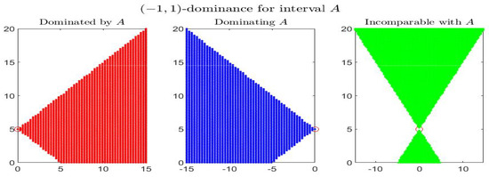
Figure 1.
-dominance (i.e., -dominance) for interval A in the midpoint-radius plane : representation of the set of dominated (red), dominating (blue) and incomparable (green) intervals.
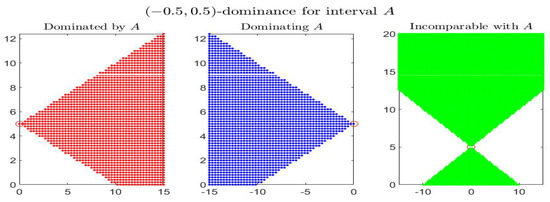
Figure 2.
-dominance for interval A in the midpoint-radius plane : representation of the set of dominated, dominating and incomparable intervals.
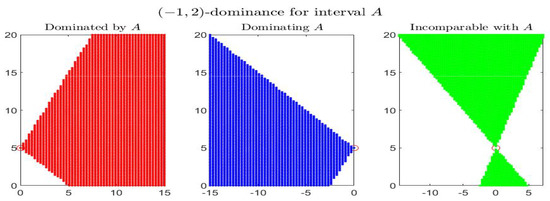
Figure 3.
-dominance for interval A in the midpoint-radius plane : representation of the set of dominated, dominating and incomparable intervals.
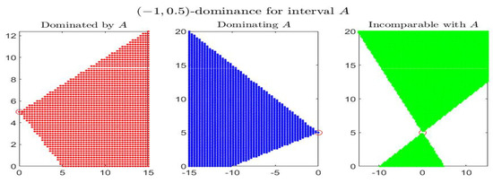
Figure 4.
-dominance for interval A in the midpoint-radius plane : representation of the set of dominated, dominating and incomparable intervals.
By inspecting the four figures, we see that with respect to the -order (Figure 1, with ) or an order with (Figure 2, with ), the set of incomparable intervals is symmetric with respect to the vertical line ; when (Figure 3) the right part of the incomparable region, determined by an increase of , tends to become more vertical and reduces in favor of the dominated region (red colored) and the dominating region (blue-colored). The opposite effect appears if decreases (Figure 4).
The lattice structure of , endowed with the partial order , can be further analyzed by considering the basic concepts of least upper bound (lub or sup) and greatest lower bound (glb or inf). For two intervals , a (common) upper bound is an interval such that and . A (common) lower bound is an interval such that and .
The least upper bound for , denoted or , is a common upper bound Z such that every other upper bound is such that ; analogously, the greatest lower bound for , denoted or , is a common lower bound Z such that every other lower bound is such that . It is immediate to see that and always exist (and are unique) for any (see [59] for details).
If is any subset of intervals, we say that is bounded from below (lower bounded) with respect to if and only if there exists such that for all and we say that is bounded from above (upper bounded) with respect to if and only if there exists such that for all . If is both lower and upper bounded, we say it is bounded.
Every bounded subset of admits inf and sup.
Proposition 8.
Consider a partial order on and let be any nonempty bounded subset of intervals. Then, there exist both such that for all
We also have, for all ,
Proof.
We will prove only Equation (15) by a constructive procedure; the proof of equations in (16) is immediate. Let be any lower bound and any upper bound for and consider the four lines, in the half-plane , with equations
They intersect the vertical axis with intercepts, respectively, , and , . Considering an arbitrary element , the two lines trough S with angular coefficients and , with equations and , respectively, have intercepts , and their sets and are both bounded with and for all . Consequently, there exist the four real numbers , , , with and . Finally, the intersection point of the two lines and corresponds to the interval ; analogously, the intersection point of the two lines and corresponds to the interval . More precisely, we have
and
This completes the proof. □
If, for a nonempty bounded subset we have that or are elements of , then there exist the intervals or, respectively, .
Interesting bounded subsets in are the “segment” with extremes and the “interval” with extremes , defined, respectively, by
and, assuming (here, the dominance is essential),
If is a bounded subset of , we clearly have , with equality if and only if with .
We conclude this section with an interesting property.
Proposition 9.
For a given partial order with , , consider the partial order ; then, for all ,
where and are the opposite intervals of A and B.
Proof.
Starting with inequalities (8) that define and recalling that the conclusion follows after a few simple algebraic manipulations. □
In particular, if , i.e., so that , we have that for any bounded subset ,
where the (bounded) subset is defined by
4. Orders in and Gh-Difference
In this section, we express a partial order in terms of the gH-difference .
Recall that from
we can write
and, for the reverse order,
Remark 3.
One may think that condition is redundant in (22); indeed, if or , it is implied by the second and third conditions. But if and , the order reduces to the standard order for real numbers while the second and the third conditions reduce to inequalities and . For this reason we will always include condition in (22). If or and the second and third conditions are both satisfied with equality, then and vice versa.
We have the following results.
Lemma 1.
Let and consider the lattice with and ; then
(1a) ⟹ (in the right part of implication, is not involved);
(1b) ⟹ (in the right part of implication, is not involved);
(2) ;
(3) Assuming , then .
Proof.
For an interval X we have that if and only if ( and ) and if and only if ( and ); the conclusion follows from the definition of and from equality . □
Remark 4.
Considering the distinction between type (i) and type (ii) of gH-difference, several other implications can be established, not used in this paper. For example in type (i), it is and we have
- -
- if and only if ;
- -
- if and only if .
Figures below show, for the given interval , the gH-differences comparing it with the corresponding set of dominated, dominating and incomparable intervals in different cases of dominance. In particular it is shown: -dominance in Figure 5, -dominance in Figure 6, -dominance in Figure 7 and -dominance in Figure 8. In all figures, the three pictures on top give the gH-differences for intervals X with and the pictures on bottom correspond to the intervals with .
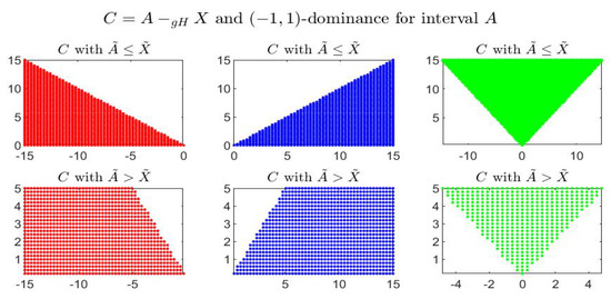
Figure 5.
-dominance for interval A: representation of the gH-differences .
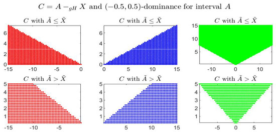
Figure 6.
-dominance for interval A: representation of the gH-differences .
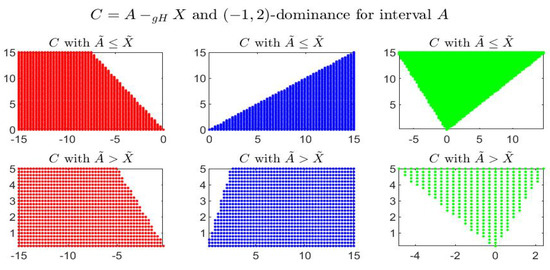
Figure 7.
-dominance for interval A: representation of the gH-differences .
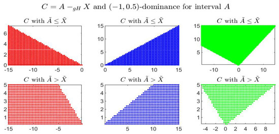
Figure 8.
-dominance for interval A: representation of the gH-differences .
In Figure 7 and Figure 8 we have and the incomparable sets are not symmetric with respect to the vertical line . In this cases, indeed, gH-differences are differently asymmetric and the position of with respect to 0 does not correspond uniquely to the position of X with respect to A; the distinction is determined by the midpoint values, i.e., when or .
5. Interval-Valued Functions
An interval-valued function is defined to be any with and for all . In midpoint representation, we write where is the midpoint value of interval and is the nonnegative half-length of :
so that
We will frequently use a second graphical representation of F, obtained in the half-plane , , where each interval is identified with the point and the arrows give the direction of moving the intervals for increasing .
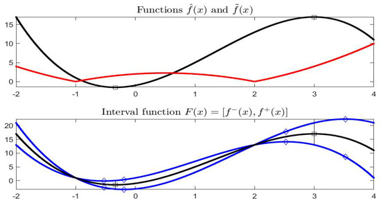
Example 1.
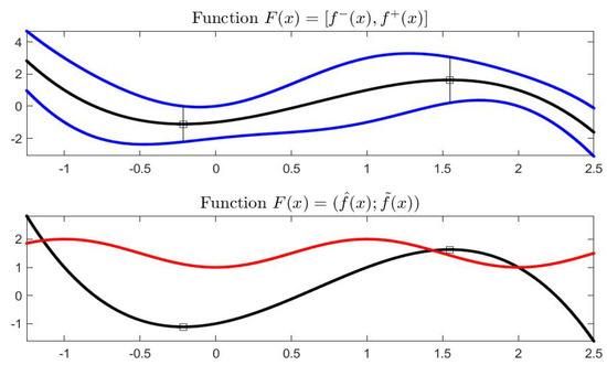
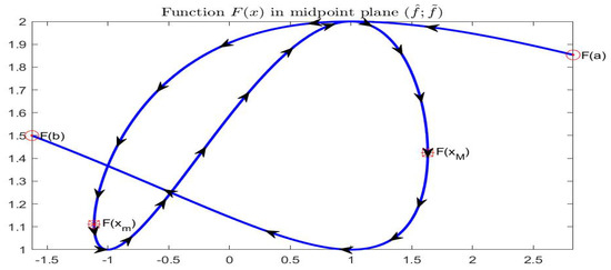
Let , in midpoint notation, i.e., , . Using the corresponding endpoint functions, the graphical representation of in the plane is given in Figure 9. For we have and for it is ; by lucking at the midpoint representation in in Figure 10, the arrows start at point and terminate at point . The values of where the midpoint function is minimal or maximal are, approximately, with interval value and with interval value .
Figure 9.
(Top) Interval-valued function in terms of endpoints functions (blue color); (bottom) function F in terms of midpoint (black color) and radius (red color).
Figure 10.
Graphical representation of F in the half-plane .
Limits and continuity can be characterized, in the Pompeiu–Hausdorff metric for intervals, by the -difference. The following result is well known [15]; the second equivalence defines the continuity at an accumulation point.
Proposition 10.
Let , , be such that and let . Let be an accumulation point of K. Then we have
where the limits are in the metric . If, in addition, , we have
Proof.
Follows immediately from the property . □
In midpoint notation, let and ; then the limits and continuity can be expressed, respectively, as
and
The following proposition connects limits to the order of intervals; we will consider the lattice with partial order defined for any fixed values of and . Analogous results can be obtained for the reverse partial order .
Proposition 11.
Let be interval-valued functions and an accumulation point for K.
- (i)
- if for all in a neighborhood of and , , then ;
- (ii)
- If for all in a neighborhood of and , then .
Proof.
We will use the midpoint notation for intervals. For the proof of i), we have if and only if and ; from (24) we have at the limit that and and this means that . For the proof of ii) we have , and , ; from , we have that exists; on the other hand, and from , we also have and so that ; the conclusion follows from (24) applied to G. □
Remark 5.
Similar results as in Propositions 10 and 11 are valid for the left limit with , ( for short) and for the right limit , ( for short); the condition that if and only if is obvious.
The gH-derivative for an interval-valued function, expressed in terms of the difference quotient by gH-difference, has been first introduced in 1979 by S. Markov (see [12]). In the fuzzy context it has been introduced in [13,62]; the interval case has been analyzed in [15] and the fuzzy case again reconsidered (level wise) in [30]. Several authors have then proposed alternative equivalent definitions and studied its properties and applications; actually, it is of interest for an increasing number of researchers. A very recent and complete description of the algebraic properties of gH-derivative can be found in [63].
Definition 10.
Let and h be such that , then the gH-derivative of a function at is defined as
if the limit exists. The interval satisfying (25) is called the generalized Hukuhara derivative of F (gH-derivative for short) at .
For the function in Example 1, we have that both and are differentiable so that exists at all internal points (see Figure 11 and Figure 12).
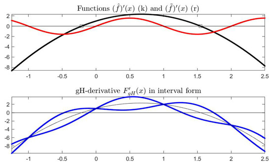
Figure 11.
Graphical representation of the derivatives and (top) and (bottom) in the plane ; the four points where is zero correspond to a singleton gH-derivative.
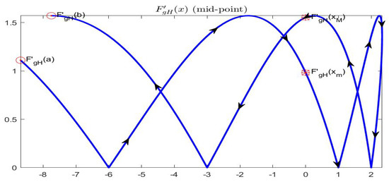
Figure 12.
Graphical representation of in the half-plane ; the two marked points (red) correspond to zeros of the derivative .
Also, one-side derivatives can be considered. The right gH-derivative of F at is while to the left it is defined as . The gH-derivative exists at if and only if the left and right derivatives at exist and are the same interval.
The following properties are indeed immediate to prove.
Proposition 12.
Let be given, . Then
- (1)
- is left gH-differentiable at if and only if and are left differentiable at ; in this case,
- (2)
- is right gH-differentiable at if and only if and are right differentiable at ; in this case, .
- (3)
- is gH-differentiable at if and only if is differentiable and is left and right differentiable at with and in this case, ; equivalently, if and only if .
In terms of midpoint representation we can write
and taking the limit for , we obtain the gH-derivative of F, if and only if the two limits and exist in ; remark that the midpoint function is required to admit the ordinary derivative at x. With respect to the existence of the second limit, the existence of the left and right derivatives and is required with (in particular if exists) so that we have
or, in the standard interval notation,
Equation (26) is of help in the interpretation of gH-derivative; indeed, the separation of midpoint and half-length components in is inherited by the gH-derivative . In particular, the correspondence
shows that the midpoint derivative is the derivative of the midpoint while the half-length derivative is the absolute value of the left and right derivatives of the half-length (with , for details see [33,35]).
For a function , we can define the gH-comparison index-function of by
If has gH-derivative at x, we can consider the gH-comparison index of at x, given by
and if , the ratio
is well defined so that ( if , if , if ). We can use the index extensively, to valuate the order relations and similar.
The partial order can be appropriately introduced for the gH-derivative by the inequality , i.e., ; if and are differentiable, we have and the inequality is equivalent to
If is not differentiable or if its left and right derivatives do not have the same absolute value, then does not exist, but possibly the left and right gH-derivatives , exist and we have , , where and are the notations for left and right derivatives. In this case, the inequalities are equivalent to
and the inequalities are equivalent to
Observe that if , then the other conditions in (29) and (30) become so that ; as a consequence, if and , then we cannot have neither nor , i.e., and 0 are incomparable.
Remark 6.
As we have seen, the existence of gH-derivative is equivalent to the existence (and their equality) of both the left and right gH-derivatives, defined as follows
and
indeed, we have and .
In many cases, the midpoint function is defined as where is differentiable; then, if also exists, we have that is gH-differentiable and .
6. Monotonicity of Functions with Values in
Monotonicity of interval-valued functions has not been much investigated and this is partially due to the lack of unique meaningful definition of an order for interval-valued functions. By definition of the lattice , endowed with the partial order ( and ) and with use of the reverse order , we can analyze monotonicity and, using the gH-difference, related characteristics of inequalities for intervals.
Definition 11.
Let be given, . We say that F is
(a-i) -nondecreasing on if implies for all ;
(a-ii) -nonincreasing on if implies for all ;
(b-i) (strictly) -increasing on if implies for all ;
(b-ii) (strictly) -decreasing on if implies for all ;
(c-i) (strongly) -increasing on if implies for all ;
(c-ii) (strongly) -decreasing on if implies for all .
If one of the six conditions is satisfied, we say that F is monotonic on ; the monotonicity is strict if (b-i,b-ii) or strong if (c-i,c-ii) are satisfied.
The monotonicity of can be analyzed also locally, in a neighborhood of an internal point , by considering condition (or condition ) for and with a positive small .
Definition 12.
Let be given, and . Let (for positive δ) denote a neighborhood of . We say that F is (locally)
(a-i) -nondecreasing at if implies for all and some ;
(a-ii) -nonicreasing at if implies for all and some ;
(b-i) (strictly)-increasing at if implies for all and some ;
(b-ii) (strictly)-decreasing at if implies for all and some ;
(c-i) (strongly) -increasing at if implies for all and some ;
(c-ii) (strongly) -decreasing at if implies for all and some .
We have if and only if , and , i.e., for increasing case,
so that is -monotonic at according to the monotonicity of the three functions , and :
Proposition 13.
Let be given, and . Then
- (i)
- is -nondecreasing at if and only if is nondecreasing, is nonincreasing and is nondecreasing at ;
- (ii)
- is -nonincreasing at if and only if is nonincreasing, is nondecreasing and is nonincreasing at .
Analogous conditions are valid for strict and strong monotonicity.
The following scheme summarizes these results:
Remark 7.
In terms of the endpoint functions and , given by , , the conditions in (32) are written as
and the conditions on and , for the monotonicity of F are less intuitive than the ones on and :
Analogously, for F to be -nonincreasing at , we obtain
Suppose now that and have both left and right (finite) derivatives at ; denote them by , , , . Taking the limits in (34) and (35) with and , we obtain the conditions for -monotonicity of F at :
Proposition 14.
Let be given, and assume that and have left and right derivatives at an internal point . The following are necessary conditions for local monotonicity:
(i-n) If F is -nondecreasing or -increasing at , then
(ii-n) If F is -nonincreasing or -decreasing at , then
The following are sufficient conditions for local strong monotonicity:
(i-s) If
then F is strongly -increasing at ;
(ii-s) If
then F is strongly -decreasing at .
If and exist on , then the conditions for monotonicity can be expressed in the obvious way as for elementary calculus, in terms of the derivatives , and . Therefore, the necessary conditions for nonincreasing are
and for nondecreasing are
With reference to Example 1, the functions , and are pictured in Figure 13 and their derivatives are in Figure 14; the partial order is fixed with and , i.e., .
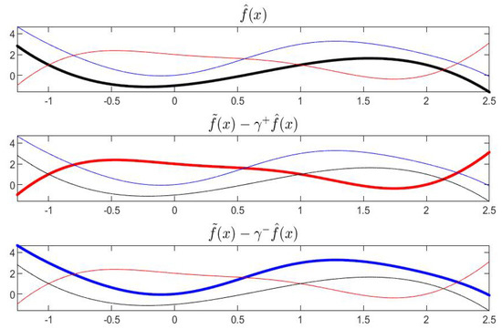
Figure 13.
Functions , and in Example 1.
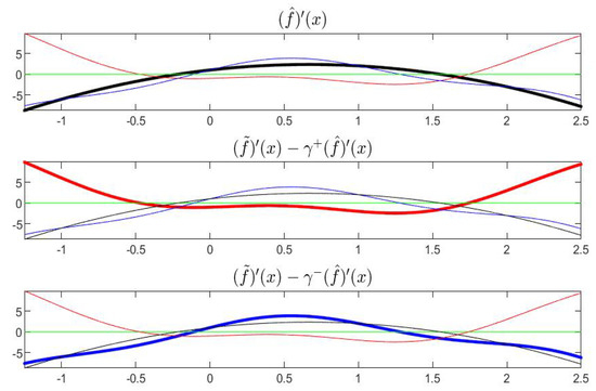
Figure 14.
Derivatives of functions , and in Example 1.
Now, but only for the case of a partial order with the condition that , i.e., , we can establish a strong connection between the monotonicity of F and the sign of its gH-derivative . Denote the corresponding partial order simply by .
Proposition 15.
Let be given, and assume F has gH-derivative at the internal points . Let be fixed. Then
- (1)
- If F is -nondecreasing on , then for all x, ;
- (2)
- If F is -nonincreasing on , then for all x, .
Proof.
We prove only (i). By definition, and F is continuous. If F is nondecreasing, then, for sufficiently small we have and so which gives; by taking the limit for , . On the other hand, for , we have , i.e., which gives; by taking the limit for we get and, changing sign on both sides, it is . The proof of (ii) is similar. □
An analogous result is also immediate, relating strong (local) monotonicity of F to the “sign” of its left and right derivatives and ; at the extreme points of , we consider only right (at a) or left (at b) monotonicity and right or left derivatives. Again we assume the condition .
Proposition 16.
Let be given, with left and/or right gH-derivatives at a point . Then
(i.a) if , then F is strongly -increasing on for some (here );
(i.b) if , then F is strongly -increasing on for some (here );
(ii.a) if , then F is strongly -decreasing on for some (here );
(ii.b) if , then F is strongly -decreasing on for some (here ).
Proof.
We prove only (i.a). From we have and , i.e., ; then , and the conclusion follows from conditions (38). □
We conclude this section with the following
Example 2.
Function , , for , is defined by and (Figure 15).
Figure 15.
(Top) functions (black) and (red); (Bottom) interval function .
Remark that function is differentiable on with and is differentiable with for and ; at these two points the left and right derivatives exist: , , , .
Function is gH-differentiable on (including the points and ) and (Figure 16). Also right and left gH-derivatives exist at and , respectively. Considering the points , , and , the corresponding gH-derivatives are (approximately) , , , .
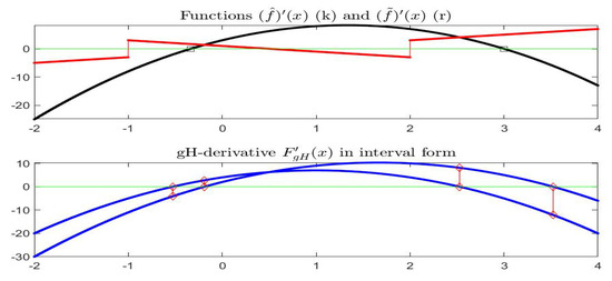
Figure 16.
(Top) derivatives of at all points (black) and of at and (red); (Bottom) gH-derivative of function ; points , , are marked in red color.
With , i.e., with ()-order, the functions , and are pictured in Figure 17.
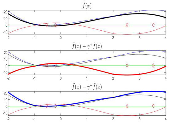
Figure 17.
Functions , and in Example 2.
According to Proposition 13, necessary conditions for decreasing are satisfied on and and for increasing are satisfied on . Corresponding necessary conditions using the sign of the derivatives of functions , and can be checked in Figure 18; at the points and we can apply the conditions involving left and right derivatives of .
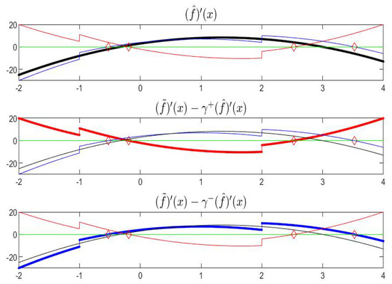
Figure 18.
Derivatives of functions , and in Example 2.
Finally, according to Proposition 16, it is easy to check that the sufficient conditions for strong monotonicity are satisfied: decreasing on and , increasing on . In the remaining points and the sufficient conditions for strong monotonicity are not satisfied (the interval-valued gH-derivatives of contain zero as an interior value).
7. Conclusions and Further Work
In the first part of this work we have introduced a general framework for ordering intervals, using a comparison index based on gH-difference; the suggested approach includes most of the partial orders proposed in the literature and preserves important desired properties, including that the space of real intervals is a lattice with the bounded property (all bounded sets of intervals have a supremum and an infimum interval).
The monotonicity properties are defined and analyzed in terms of the suggested partial orders and the relevant connections with gH-derivative are established.
In Part II of the paper, we will further develop new results to define extremal points (local or global minimum or maximum) in terms of the same general partial orders developed in this part and we will analyze the important concepts of concavity and convexity by the use of first-order and second-order gH-derivatives.
Interesting connections with differential geometry and with periodic curves (as in [64,65,66]) will be analyzed.
Author Contributions
The authors contributed equally in writing the manuscript.
Funding
This research received no external funding.
Conflicts of Interest
The authors declare no conflict of interest.
References
- Alefeld, G.; Herzberger, J. Introduction to Interval Computations; Academic Press: New York, NY, USA, 1983. [Google Scholar]
- Alefeld, G.; Mayer, G. Interval analysis: Theory and applications. J. Comput. Appl. Math. 2000, 121, 421–464. [Google Scholar] [CrossRef]
- Jaulin, L.; Kieffer, M.; Didrit, O. Applied Interval Analysis; Springer: Berlin/Heidelberg, Germany, 2006. [Google Scholar]
- Markov, S. On the Algebra of Intervals. Reliab. Comput. 2016, 21, 80–108. [Google Scholar]
- Moore, R.E. Interval Analysis; Prentice-Hall: Englewood Cliffs, NJ, USA, 1966. [Google Scholar]
- Moore, R.E. Method and Applications of Interval Analysis; SIAM: Philadelphia, PA, USA, 1979. [Google Scholar]
- Moore, R.E.; Kearfott, R.B.; Cloud, M.J. Introduction to Interval Analysis; SIAM: Philadelphia, PA, USA, 2009. [Google Scholar]
- Althoff, M.; Grebenyuk, D. Implementation of Interval Arithmetic in CORA 2016 (Tool Presentation). Ser. Comput. 2017, 43, 91–105. [Google Scholar]
- Banks, H.T.; Jacobs, M.Q. A differential calculus for multi-functions. J. Math. Anal. Appl. 1970, 29, 246–272. [Google Scholar] [CrossRef]
- Hukuhara, M. Integration des applications mesurables dont la valeur est un compact convexe. Funkc. Ekvacioj 1967, 10, 205–223. [Google Scholar]
- Puri, M.L.; Ralescu, D.A. Differentials for fuzzy functions. J. Math. Anal. Appl. 1983, 91, 552–558. [Google Scholar] [CrossRef]
- Markov, S. Calculus for interval functions of real variable. Computing 1979, 22, 325–337. [Google Scholar] [CrossRef]
- Stefanini, L. A generalization of Hukuhara difference. In Soft Methods for Handling Variability and Imprecision; Springer: Berlin/Heidelberg, Germany, 2008; pp. 205–210. [Google Scholar]
- Stefanini, L. A generalization of Hukuhara difference and division for interval and fuzzy arithmetic. Fuzzy Sets Syst. 2010, 161, 1564–1584. [Google Scholar] [CrossRef]
- Stefanini, L.; Bede, B. Generalized Hukuhara differentiability of interval-valued functions and interval differential equations. Nonlinear Anal. 2009, 71, 1311–1328. [Google Scholar] [CrossRef]
- Dubois, D.; Prade, H. Fuzzy Sets and Systems: Theory and Applications; Academic Press: New York, NY, USA, 1980. [Google Scholar]
- Dubois, D.; Prade, H. Fundamentals of Fuzzy Sets; The Handbooks of Fuzzy Sets Series; Kluwer: Boston, MA, USA, 2000. [Google Scholar]
- Floudas, C.A.; Pardalos, P.M. Encyclopedia of Optimization; Springer: Berlin/Heidelberg, Germany, 2009. [Google Scholar]
- Goestschel, R.; Voxman, W. Elementary fuzzy calculus. Fuzzy Sets Syst. 1986, 18, 31–43. [Google Scholar] [CrossRef]
- Lodwick, W.A.; Kacprzyk, J. Fuzzy Optimization. Recent Advances and Applications; Springer: Berlin/Heidelberg, Germany, 2010. [Google Scholar]
- Negoita, C.V.; Ralescu, D. Applications of Fuzzy Sets to Systems Analysis; Birkhauser Verlag: Basel, Switzerland, 1975. [Google Scholar]
- Roedder, W.; Zimmermann, H.-J. Duality in Fuzzy Linear Programming. In Extremal Theory for Systems Analysis; Fiacco, A.V., Kortanek, K., Eds.; Springer: Berlin/Heidelberg, Germany, 1980; pp. 415–429. [Google Scholar]
- Slowinski, R. Fuzzy Sets in Decision Analysis, Operations Research and Statistics, Part II; Springer: Berlin/Heidelberg, Germany, 1998; pp. 179–309. [Google Scholar]
- Tanaka, H.; Okuda, T.; Asai, K. On Fuzzy Mathematical Programming. J. Cybern. 1974, 3, 37–46. [Google Scholar] [CrossRef]
- Tong, S. Interval number and fuzzy number linear programming. Fuzzy Sets Syst. 1994, 66, 301–306. [Google Scholar]
- Verdegay, J.L. A dual approach to solve the fuzzy linear programming problem. Fuzzy Sets Syst. 1984, 14, 131–141. [Google Scholar] [CrossRef]
- Verdegay, J.L. Progress on Fuzzy Mathematical Programming: A personal perspective. Fuzzy Sets Syst. 2015, 281, 219–226. [Google Scholar] [CrossRef]
- Zimmermann, H.-J. Fuzzy programming and linear programming with several objective functions. Fuzzy Sets Syst. 1978, 1, 45–55. [Google Scholar] [CrossRef]
- Zimmermann, H.J. Fuzzy Sets, Decision Making and Expert Systems; Kluwer-Nijhoff: Boston, MA, USA, 1987. [Google Scholar]
- Bede, B.; Stefanini, L. Generalized differentiability of fuzzy-valued functions. Fuzzy Sets Syst. 2013, 230, 119–141. [Google Scholar] [CrossRef]
- Chalco-Cano, Y.; Lodwick, W.A.; Rufian-Lizana, A. Optimality conditions of type KKT for optimization problem with interval-valued objective function via generalized derivative. Fuzzy Optim. Decis. Mak. 2013, 12, 305–322. [Google Scholar] [CrossRef]
- Chalco-Cano, Y.; Román-Flores, H.; Jiménez-Gamero, M.D. Generalized derivative and π-derivative for set-valued functions. Inf. Sci. 2011, 181, 2177–2188. [Google Scholar] [CrossRef]
- Chalco-Cano, Y.; Rufian-Lizana, A.; Roman-Flores, H.; Jimenez-Gamero, M.D. Calculus for interval-valued functions using generalized Hukuhara derivative and applications. Fuzzy Sets Syst. 2013, 219, 49–67. [Google Scholar] [CrossRef]
- Chalco-Cano, Y.; Rufian-Lizana, A.; Roman-Flores, H.; Osuna-Gomez, R. A note on generalized convexity for fuzzy mappings through a linear ordering. Fuzzy Sets Syst. 2013, 231, 70–83. [Google Scholar] [CrossRef]
- Stefanini, L.; Arana-Jimenez, M. Karush-Kuhn-Tucker conditions for interval and fuzzy optimization in several variables under total and directional generalized differentiability. Fuzzy Sets Syst. 2019, 362, 1–34. [Google Scholar] [CrossRef]
- Stefanini, L.; Bede, B. Generalized fuzzy differentiability with LU-parametric representations. Fuzzy Sets Syst. 2014, 257, 184–203. [Google Scholar] [CrossRef]
- Bede, B. Mathematics of Fuzzy Sets and Fuzzy Logic; Series: Studies in Fuzziness and Soft Computing n. 295; Springer: Berlin/Heidelberg, Germany, 2013. [Google Scholar]
- Bede, B.; Gal, S.G. Generalizations of the differentiability of fuzzy-number-valued functions with applications to fuzzy differential equations. Fuzzy Sets Syst. 2005, 151, 581–599. [Google Scholar] [CrossRef]
- Bede, B.; Rudas, I.J.; Bencsik, A. First order linear differential equations under generalized differentiability. Inf. Sci. 2007, 177, 1648–1662. [Google Scholar] [CrossRef]
- Alolyan, I. Algorithm for Interval Linear Programming Involving Interval Constraints. In Proceedings of the WCECS 2013 Conference, Edmonton, AB, Canada, 24–28 June 2013. [Google Scholar]
- Allahdadi, M.; Nehi, H.M.; Ashayerinasab, H.A.; Javanmard, M. Improving the modified interval linear programming method by new techniques. Inf. Sci. 2016, 339, 224–236. [Google Scholar] [CrossRef]
- Bellman, R.E.; Zadeh, L.E. Decision making in a fuzzy environment. Manag. Sci. 1970, 17, B141–B164. [Google Scholar] [CrossRef]
- Chalco-Cano, Y.; Lodwick, W.A.; Osuna-Gomez, R.; Rufian-Lizana, A. The Karush-Kuhn-Tucker optimality conditions for fuzzy optimization problems. Fuzzy Optim. Decis. Mak. 2016, 15, 57–73. [Google Scholar] [CrossRef]
- Despotis, D.K.; Smirlis, Y.G. Data envelopment analysis with imprecise data. Eur. J. Oper. Res. 2002, 140, 24–36. [Google Scholar] [CrossRef]
- Inuiguchi, M.; Kume, Y. Goal programming problems with interval coefficients and target intervals. Eur. J. Oper. 1991, 52, 345–360. [Google Scholar] [CrossRef]
- Inuiguchi, M.; Ramik, J.; Tanino, T.; Vlach, M. Satisficing solutions and duality in interval and fuzzy linear programming. Fuzzy Sets Syst. 2003, 135, 151–177. [Google Scholar] [CrossRef]
- Ishibuchi, H.; Tanaka, H. Multiobjective programming in optimization of the interval objective function. Eur. J. Oper. Res. 1990, 48, 219–225. [Google Scholar] [CrossRef]
- Mostafaee, A.; Černý, M. Inverse linear programming with interval coefficients. J. Comput. Appl. Math. 2016, 292, 591–608. [Google Scholar] [CrossRef]
- Osuna-Gomez, R.; Chalco-Cano, Y.; Hernandez-Jimenez, B.; Ruiz-Garzon, G. Optimality conditions for generalized differentiable interval-valued functions. Inf. Sci. 2015, 321, 136–146. [Google Scholar] [CrossRef]
- Osuna-Gomez, R.; Chalco-Cano, Y.; Rufián-Lizana, A.; Hernandez-Jimenez, B. Necessary and sufficient conditions for fuzzy optimality problems. Fuzzy Sets Syst. 2016, 296, 112–123. [Google Scholar] [CrossRef]
- Sun, J.; Gong, D.; Zeng, X.; Geng, N. An ensemble framework for assessing solutions of interval programming problems. Inf. Sci. 2018, 436–437, 146–161. [Google Scholar] [CrossRef]
- Wu, H.C. The Karush-Kuhn-Tucker optimality conditions in an optimization problem with interval-valued objective function. Eur. J. Oper. Res. 2007, 176, 46–59. [Google Scholar] [CrossRef]
- Wu, H.C. The Karush-Kuhn-Tucker optimality conditions in multiobjective programming problems with interval-valued objective functions. Eur. J. Oper. Res. 2009, 196, 49–60. [Google Scholar] [CrossRef]
- Wu, H.C. The optimality conditions for optimization problems with convex constraints and multiple fuzzy-valued objective functions. Fuzzy Optim. Decis. Mak. 2009, 8, 295–321. [Google Scholar] [CrossRef]
- Wu, H.C. Duality theory in interval-valued linear programming problems. Optim. Theory Appl. 2011, 150, 298–316. [Google Scholar] [CrossRef]
- Guerra, M.L.; Sorini, L.; Stefanini, L. A new approach to linear programming with interval costs. In Proceedings of the FUZZ-IEEE 2017 Conference, Naples, Italy, 9–12 July 2017. [Google Scholar]
- Stefanini, L.; Bede, B. A new gH-difference for multi-dimensional convex sets and convex fuzzy sets. Axioms 2019, 8, 48. [Google Scholar] [CrossRef]
- Guerra, M.L.; Stefanini, L. A comparison index for interval ordering. In Proceedings of the IEEE SSCI 2011, Symposium series on Computational Intelligence (FOCI 2011), Paris, France, 11–15 April 2011; pp. 53–58. [Google Scholar]
- Guerra, M.L.; Stefanini, L. A comparison index for interval ordering based on generalized Hukuhara difference. Soft Comput. 2012, 16, 1931–1943. [Google Scholar] [CrossRef]
- Sengupta, A.; Pal, T.K. On comparing interval numbers. Eur. J. Oper. Res. 2000, 127, 28–43. [Google Scholar] [CrossRef]
- Sengupta, A.; Pal, T.K. Fuzzy Preference Ordering of Interval Numbers in Decision Problems; Springer: Berlin/Heidelberg, Germany, 2009. [Google Scholar]
- Stefanini, L. On the generalized LU-fuzzy derivative and fuzzy differential Equations. In Proceedings of the IEEE International Fuzzy Systems Conference, London, UK, 23–26 July 2007. [Google Scholar] [CrossRef]
- Chalco-Cano, Y.; Maqui-Huaman, G.G.; Silva, G.N.; Jiménez-Gamero, M.D. Algebra of generalized Hukuhara differentiable interval-valued functions: review and new properties. Fuzzy Sets Syst. 2019, 375, 53–69. [Google Scholar] [CrossRef]
- Gray, A.; Abbena, E.; Salamon, S. Modern Differential Geometry of Curves and Surfaces with Mathematica, 3rd ed.; CRC Press: Boca Raton, FL, USA, 2006. [Google Scholar]
- Rovenski, V. Modeling of Curves and Surfaces with MATLAB; Springer: Berlin/Heidelberg, Germany, 2010. [Google Scholar]
- Baer, C. Elementary Differential Geometry; Cambridge University Press: Cambridge, UK, 2010. [Google Scholar]


© 2019 by the authors. Licensee MDPI, Basel, Switzerland. This article is an open access article distributed under the terms and conditions of the Creative Commons Attribution (CC BY) license (http://creativecommons.org/licenses/by/4.0/).