Fault Feature Enhanced Extraction and Fault Diagnosis Method of Vibrating Screen Bearings

Abstract

For mechanical equipment, bearings have a high incidence area of faults. A problem for bearings is that their fault characteristics include a vibrating screen exciter which is weak and thus easily covered in strong background noise, hence making the noise difficult to remove. In this paper, a noise reduction method based on singular value decomposition, improved by singular value’s unilateral ascent method (SSVD), and a fault feature enhancement method, i.e., variational mode decomposition, improved by revised whale algorithm optimization (RWOA-VMD), are proposed. These two methods are used in vibration signal processing with early faults of bearings having a vibrating screen and they have achieved significant application results. This paper also aims to construct a multi-modal feature matrix composed of energy entropy, singular value entropy, and power spectrum entropy, and then the early fault diagnosis of bearings of a vibrating screen exciter bearing is realized by using the proposed support vector machine, improved by the aquila optimizer algorithm (AO-SVM).

1. Introduction

As an important part of vibrating machinery, large-sized vibrating screens have been widely used, especially in the fields of coal preparation and recycling utilization of construction waste. Large disposal capacity, which has reached more than 2000 t/h [1], and poor working conditions lead to high failure rates. In particular, due to the comprehensive influence of large clearance, spring support, and alternating excitation, the dynamic coupling reaction between the internal parts of the exciter is strong. That is, the collision is more frequent, the friction is aggravated, and fatigue failure is very prone to occur. Therefore, bearing failures account for the highest proportion of exciter failures. Due to the early failure of the weak bearing itself, submerged in the strong reciprocating vibration of the exciter, early fault feature extraction of the bearing is more difficult, which poses a greater challenge for the early fault diagnosis of the bearing for the vibrating screen exciter.

At present, common signal processing methods include short-time Fourier transform, wavelet transform, empirical mode decomposition, and some other mode decomposition algorithms. Due to the problem of the window function, the time-frequency resolution of the short-time Fourier transform cannot be adjusted adaptively [2]. Because of the selection of wavelet bases, the wavelet transform has the problem of insufficient adaptability [3]. Therefore, the most popular method of time-frequency analysis in recent studies is the adaptive signal decomposition method [4]. The most commonly used adaptive mode decomposition methods are empirical mode decomposition (EMD), ensemble empirical mode decomposition (EEMD) [5], empirical wavelet transform (EWT) [6], and variational mode decomposition (VMD) [7]. EMD is widely used in various fields, but it has difficulty in mathematical modeling, noise sensitivity, and endpoint effects. EEMD overcomes the mode aliasing of EMD, but it takes too long and does not overcome the endpoint effect [8]. Many scholars had studied EWT [9,10,11,12], compared with EMD, the EWT method effectively suppresses the endpoint effect and mode aliasing phenomenon [13], and because EWT adopts a non-recursive decomposition method, it greatly improved the computational efficiency [14]. However, the effect of EWT on boundary detection in Fourier spectroscopy is not good [15]. VMD not only overcomes the shortcomings of endpoint effect and mode aliasing, but also has a solid mathematical foundation; however, its parameter selection cannot be well determined. Although many scholars have carried out research on it [16,17,18,19,20], there are still certain limitations.

On the aspect of fault diagnosis, detection and diagnosis of faults (FDD) have become an active issue, in which data-driven fault diagnosis applied in traction systems of high-speed trains is one of these FDD methods. Data-driven designs can be directly implemented without a logical or mathematical description of traction systems, and have thus received special attention because of their overwhelming advantages [21,22,23,24,25]. For the fault diagnosis of bearings of the vibrating screen exciter, a few scholars have conducted research. Xu and Cai [26] applied VMD improved by K-L divergence method to the extraction of fault characteristics of vibrating screen bearings; and Cai et al. [27] proposed an envelope derivative energy operator (EDO). The aforementioned researches focus on the extraction of bearing fault features of bearings of vibrating screen exciter, but they do not propose a fault identification method to carry out intelligent diagnosis of early faults.

In summary, it is necessary to further study the enhanced extraction of early fault features and the intelligent fault diagnosis algorithm of the bearings of the vibrating screen. The remainder of this paper is organized as follows. Section 2 proposes a singular value decomposition improved by singular value’s unilateral ascent method (SSVD) for signal noise reduction. In Section 3, the revised whale algorithm is used to improve the variational mode decomposition (RWOA-VMD) to enhance the application effect of fault feature extraction. Section 4 discusses the combined application of SSVD and RWOA-VMD to the bearing signal analysis of the vibrating screen exciter. Section 5 puts forward the energy entropy, singular value entropy, and power spectrum entropy of the combined processed signal in Section 4 as multi-modal features, and then proposes an improved support vector machine based on the aquila optimizer algorithm (AO-SVM) to enhance the early fault diagnosis accuracy of bearings of the vibrating screen exciter. Conclusions are drawn in Section 6.

2. Improved Singular Value Decomposition Based on Singular Value’s Unilateral Ascent Rate Method (SSVD) for Pre-Denoising

2.1. Signal Reconstruction Principle Based on Singular Value’s Unilateral Ascent Rate Method

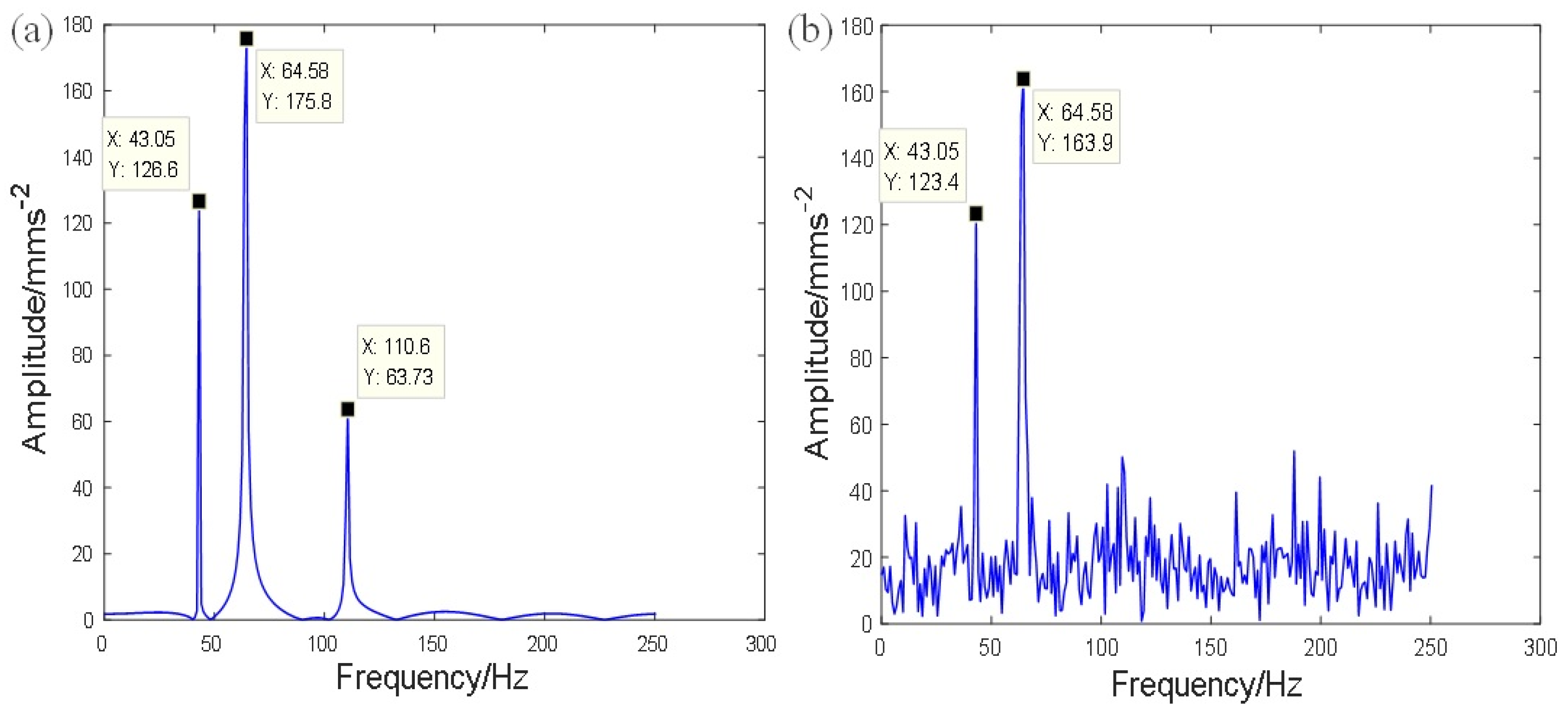
First, a discrete signal x is constructed into the Hankel Matrix, and the delay step is 1, that is, the data of each row (column) lags behind the data of the previous row (column) by 1. Then, the corresponding m × n matrix is obtained:

$$A_{m\times n}=\left[\begin{array}{cccc}{x}_1& x_2& \cdots & x_n\\ x_2& x_3& \cdots & x_{n+1}\\ ⋮& ⋮& \ddots & ⋮\\ x_m& x_{m+1}& \cdots & x_N\end{array}\right]$$

(1)

where, $n=N-m+1$.

A sequence of singular values $S_1=\left[{\sigma }_1,{\sigma }_2,{\sigma }_3,\cdots ,{\sigma }_r\right]$ are derived from the Hankel matrix $A_{m\times n}$ for the discrete signal x. ${\sigma }_1$ represents the $r$th singular value. The instantaneous ascent rate is defined as:

$$V_i={\sigma }_i-{\sigma }_{i-1}$$

(2)

The average ascent rate of all singular values is defined as:

$$V_{1,r}=\left({\sigma }_1-{\sigma }_r\right)/\left(r-1\right)$$

(3)

The singular values are arranged from small to large, and the difference between the instantaneous ascent rate and the average ascent rate of all singular values is defined as:

$$C_i=V_i-V_{1,r}\left(i=1,2,\dots ,r\right)$$

(4)

Singular values can reflect the energy concentration of signal and noise. Larger singular values reflect useful signals, while the smaller values mainly represent noise. Since the size difference of the latter is small, the instantaneous ascent rate of singular values reflecting noise is significantly smaller than the average ascent rate of all singular values $V_{1,r}$, that is, $C_i\le 0$. When the singular value increases to a certain extent, that is, its instantaneous ascent rate begins to have a significant change, i.e., $C_i\ge 0$. Singular values satisfying $C_i\ge 0$ are equivalent to peak values derived from another noise reduction method, namely, singular value difference spectra. However, the information carried by peak values may not be useful information needed, which results in poor noise reduction effect based on the singular value difference spectra. To solve this problem, this paper proposes that only when the singular value rises at the fastest rate can the optimal number of singular values be selected, and this point is called the $k$ point, that is:

$$C_k=\mathit{max}(C_1,C_2,\dots ,C_r)$$

(5)

Therefore, the optimal number of singular values for signal reconstruction is selected as $k$ point and the subsequent point, that is, $k$~$r$. Therefore, this method cannot only avoid insufficient noise reduction, but it can also avoid over-noise reduction.

The signal reconstruction method selected by this principle is called improved singular value decomposition based on singular value’s unilateral ascent rate method (SSVD). This method cannot only effectively remove the noise, but also avoid the phenomenon of over-noise reduction.

2.2. Simulation

To verify the effectiveness of the singular value’s unilateral ascent method, the simulated signal $x\left(t\right)$ is constructed as:

$$x\left(t\right)=\mathit{cos}\left(128\pi t\right)+0.5\times \mathit{cos}\left(86\pi t\right)+0.3\times \mathit{cos}\left(220\pi t\right)$$

(6)

where the sampling frequency $f_s=500\mathrm{Hz}$ and sampling time $t=1\mathrm{s}$. A Gaussian white noise with $SNR=1$ is added to the simulated signal to simulate the strong noise under actual working conditions. Frequency spectrums with and without noise are, respectively, shown in Figure 1. It can be found that one signal component is overwhelmed in the strong noise.

The effective number of singular values is obtained by using SSVD, as shown in Figure 2a. At the point $k=245$, the difference $C_k$ between the instantaneous ascent rate and the average ascent rate is the maximum, so the singular value points from 245 to 260 are selected for signal reconstruction. The frequency spectrum after noise reduction by SSVD preserves the three frequency components of the original signal while greatly eliminating the noise in the signal.

In order to prove the advantage of SSVD in denoising, one commonly used method of selecting effective singular values based on the singular value difference spectrum is compared with SSVD here. According to the principle of the singular value difference spectrum, as shown in Figure 2b, the maximum point of the difference spectrum appears at point $k=2$, so the first two singular value points are selected to reconstruct the signal; however, two frequency components are obviously missing. So, this method is easy to cause excessive noise reduction. Therefore, SSVD has a better noise reduction effect under strong background noise.

3. Variational Mode Decomposition Improved by Revised Whale Optimization Algorithm (RWOA-VMD) for Fault FEATURE Enhancement

VMD is an adaptive and completely non recursive method of mode variation and signal processing. VMD can be summarized as: (1) updating each mode in the frequency domain, and then converting the signal from the frequency domain to the time domain through the inverse Fourier transform; (2) the central frequency of each IMF component is continuously re-evaluated. The specific process of the algorithm iteration is as follows: (1) initialize each mode $\left\{{\widehat{u}}_k^1\right\}$, center frequency $\left\{{\widehat{\omega }}_k^1\right\}$ and the number of decomposition levels $K$, where $k=1,\dots ,K$; (2) update $u_k$ and ${\omega }_k$ according to equations: ${\widehat{u}}_k^{n+1}\left(\omega \right)=\frac{\widehat{f}\left(\omega \right)-{{\displaystyle \sum }}_{i\ne k}{\widehat{u}}_i\left(\omega \right)+\frac{\widehat{\lambda }\left(\omega \right)}{2}}{1+2\alpha {\left(\omega -{\omega }_k\right)}^2}$ and ${\widehat{\omega }}_k^{n+1}=\frac{{{\displaystyle \int }}_0^{\infty }\omega {\left|{\widehat{u}}_k\left(\omega \right)\right|}^{2}d\omega }{{{\displaystyle \int }}_0^{\infty }{\left|{\widehat{u}}_k\left(\omega \right)\right|}^{2}d\omega }$, where $f$ is the original input signal, $\alpha$ is penalty factor; (3) update Lagrange multiplier operator $\lambda$ according to equation ${\widehat{\lambda }}^{n+1}\left(\omega \right)={\widehat{\lambda }}^n\left(\omega \right)+\tau \left(\widehat{f}\left(\omega \right)-{\displaystyle \sum }_k{\widehat{u}}_k^{n+1}\left(\omega \right)\right)$; (4) terminate the iteration according to whether the termination conditions are met in ${\displaystyle \sum }_n\frac{\Vert u_n^{k+1}-u_n^k\Vert }{\Vert u_n^k\Vert {}_2^2}<\epsilon$ (where, determination accuracy $\epsilon <0$), if not, return to step (2). However, the application effect of VMD on false mode components inhibition and mode aliasing and endpoint effect alleviation is highly dependent on the choice of two key parameters: the number of decomposition levels $K$ and penalty factor $\alpha$. It often depends on human experience and the optimization of some algorithms. At present, human experience mostly determines $K$ through the observation of central frequency, but this method is very accidental and time-consuming. Human experience can only determine $K$, but cannot determine $\alpha$. Although some algorithms have achieved some results in optimizing VMD, there are also serious defects. The convergence precision and speed are relatively slow, and they often fall into local optimization [28]. This section will focus on the selection of the best values of these two parameters for the purpose of improvement of VMD.

3.1. Whale Optimization Algorithm (WOA)

Inspired by the foraging behavior of humpback whales, Mirjalili and Lewis [29] proposed a new meta-heuristic optimization algorithm, i.e., WOA. The algorithm is divided into three stages: initialization stage, local search stage, and global exploration stage.

① Initialization stage: Suppose that N solutions are randomly generated to form an initial population, and the predation space is D-dimensional. D-dimensional optimization problems can be described as:

$$\begin{gathered} \mathit{min}f\left(x\right) \\ s.t.l\le x\le u \end{gathered}$$

(7)

where $f\left(x\right)$ is single objective optimization function, $x\in R^D$ is an independent variable, and $u,l\in R^D$ are the upper and lower boundaries of $x$, respectively.

The initial population can be expressed as $G\left(0\right)=\left\{x_1\left(0\right),x_2\left(0\right),\dots x_N\left(0\right)\right\}$, the ith solution is $x_i\left(0\right)=\left[x_{i1}\left(0\right),x_{i2}\left(0\right),\dots x_{iD}\left(0\right)\right]$. Then, there is:

$$x_{ij}\left(0\right)=l_j+rand\left(0,1\right)\left(u_j-l_j\right)$$

(8)

where $u_j$ and $l_j$ are the upper and lower boundaries of the ith dimension, and $x_{*}\left(0\right)=arg\underset{1\le i\le N}{\mathit{min}}f\left(x_i\left(0\right)\right)$ represents the optimal individual in the population.

② Local exploration stage: the essence of the local exploration stage is a process of finding the optimal solution through the shrinking encircling mechanism and spiral updating position mechanism in the local area. The mechanism of shrink wrap is expressed as:

$$x_{ij}\left(t+1\right)=x_{*j}\left(t\right)-A{d}_{ij}\left(t\right)$$

(9)

$$A=\left(2-\frac{t}{t_{max}}\right)\left(2r-1\right)$$

(10)

where $t$ is the current number of iterations, $x_{*j}\left(t\right)$ is the position of the current best candidate solution, $d_{ij}\left(t\right)=\left|2r{x}_{*j}\left(t\right)-x_{ij}\left(t\right)\right|$, $r$ is uniformly distributed random number among $\left[-1,1\right]$, and $t_{max}$ is the maximum number of iterations.

The spiral updating position mechanism is expressed as:

$$x_{ij}\left(t+1\right)=x_{*j}\left(t\right)+e^{bl}cos\left(2\pi l\right){\tilde{d}}_{ij}\left(t\right)$$

(11)

where $b$ is a constant relating to the spiral shape, $l$ is a random number of $\left[-1,1\right]$, and ${\tilde{d}}_{ij}\left(t\right)=\left|x_{*j}\left(t\right)-x_{ij}\left(t\right)\right|$.

③ Global exploration stage

In the global exploration stage, prey search is carried out by a search agent randomly selected from the population. The whale location can be updated as:

$$x_{ij}\left(t+1\right)=x_{rj}\left(t\right)-A{d}_{ij}\left(t\right)$$

(12)

where $x_{rj}\left(t\right)$ is the $j$th dimension of a random whale, and $d_{ij}\left(t\right)=\left|2r{x}_{rj}\left(t\right)-x_{ij}\left(t\right)\right|$.

3.2. Revised Whale Optimization Algorithm (RWOA)

In order to quickly find the optimal location, each whale searches and transmits information within a specific range. Therefore, designing a suitable search radius as the search range of whales is very critical to improve the convergence speed of the algorithm to obtain the optimal solution.

For the $i$th whale in the population $x_i\left(t\right)$, calculate the distance $d_i^k\left(t\right)$ between it and the other whales in the population $x_k\left(t\right)$, $k\ne i,k=1,2,\dots ,N$:

$$d_i^k\left(t\right)=\sqrt{{\displaystyle \sum }_{j=1}^D(x_{ij}\left(t\right)-x_{kj}{\left(t\right)}^2}$$

(13)

Calculate the distance $d_i^k\left(t\right)$ between the ith whale $x_i\left(t\right)$ and other whales $x_k\left(t\right)$. The maximum distance is $c_p$, $p\ne i,p=1,2,\dots ,N$, and the minimum value is $c_q$, $q\ne i,q=1,2,\dots ,N$. $c_1$ and $c_2$ are excluded in order to reduce the error caused by extremity of the value.

$$\begin{gathered} c_p=d_i^k{\left(t\right)}_{max}=d_i^p\left(t\right) \\ {c}_q=d_i^k{\left(t\right)}_{min}=d_i^q\left(t\right) \end{gathered}$$

(14)

Define the search radius $R_i\left(t\right)$ of the ith whale as:

$$R_i\left(t\right)=\frac{{{\displaystyle \sum }}_{k=1,k\ne i,p,q}^N{d}_i^k\left(t\right)}{N-3}$$

(15)

The neighborhood of the $i$th whale $x_i\left(t\right)$ planned by the search radius $R_i\left(t\right)$ is:

$$N{b}_i\left(t\right)=\left\{x_k\left(t\right)|d_i^k\left(t\right)\le R_i\left(t\right),k\ne i,p,q,k=1,2,\dots ,N\right\}$$

(16)

Additionally, the optimal individual of N is recorded as:

$$x_i^{lbest}\left(t\right)=arg\underset{x_k\in N{b}_i}{min}f(x_k\left(t\right))$$

(17)

Under the case of $|A>1|$, the ith whale will search in the global adaptive neighborhood. In order to improve the convergence rate and overcome the problem of local optimization, Equation (12) is revised as:

$$x_{ij}\left(t+1\right)=x_{iJ}^{lbest}\left(t\right)-A{d}_{ij}\left(t\right)$$

(18)

where, $d_{ij}\left(t\right)=\left|2r{x}_{iJ}^{lbest}\left(t\right)-x_{ij}\left(t\right)\right|$.

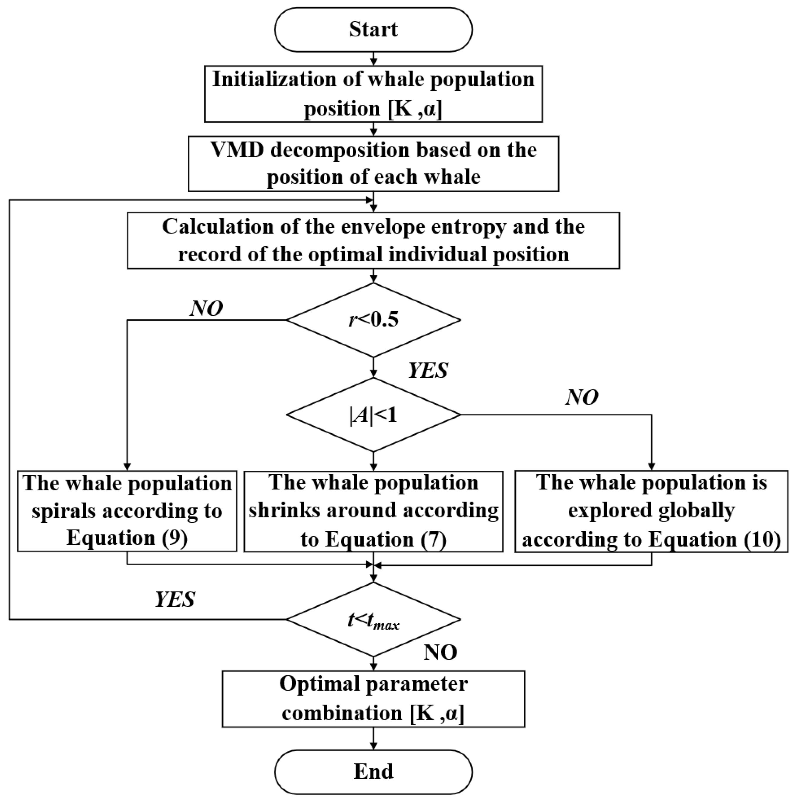
3.3. Variational Mode Decomposition Improved by Revised Whale Optimization Algorithm (RWOA-VMD)

For signal $x\left(i\right)\left(i=1,2,\dots ,N\right)$, define its envelope entropy $E_p$ as follows:

$$\{\begin{array}{c}{E}_p={\displaystyle {\displaystyle \sum }_{i=1}^N}\epsilon \left(i\right)lg\epsilon \left(i\right)\\ \epsilon \left(i\right)=a\left(i\right)/{\displaystyle {\displaystyle \sum }_{i=1}^N}a\left(i\right)\end{array}$$

(19)

where $N$ is the number of sampling points, $a\left(i\right)$ is the signal demodulated by Hilbert, and $\epsilon \left(i\right)$ is the normalized probability distribution sequence of $a\left(i\right)$.

In the following content, WOA will be used to further improve VMD, namely RWOA-VMD, and its flowchart is shown in Figure 3.

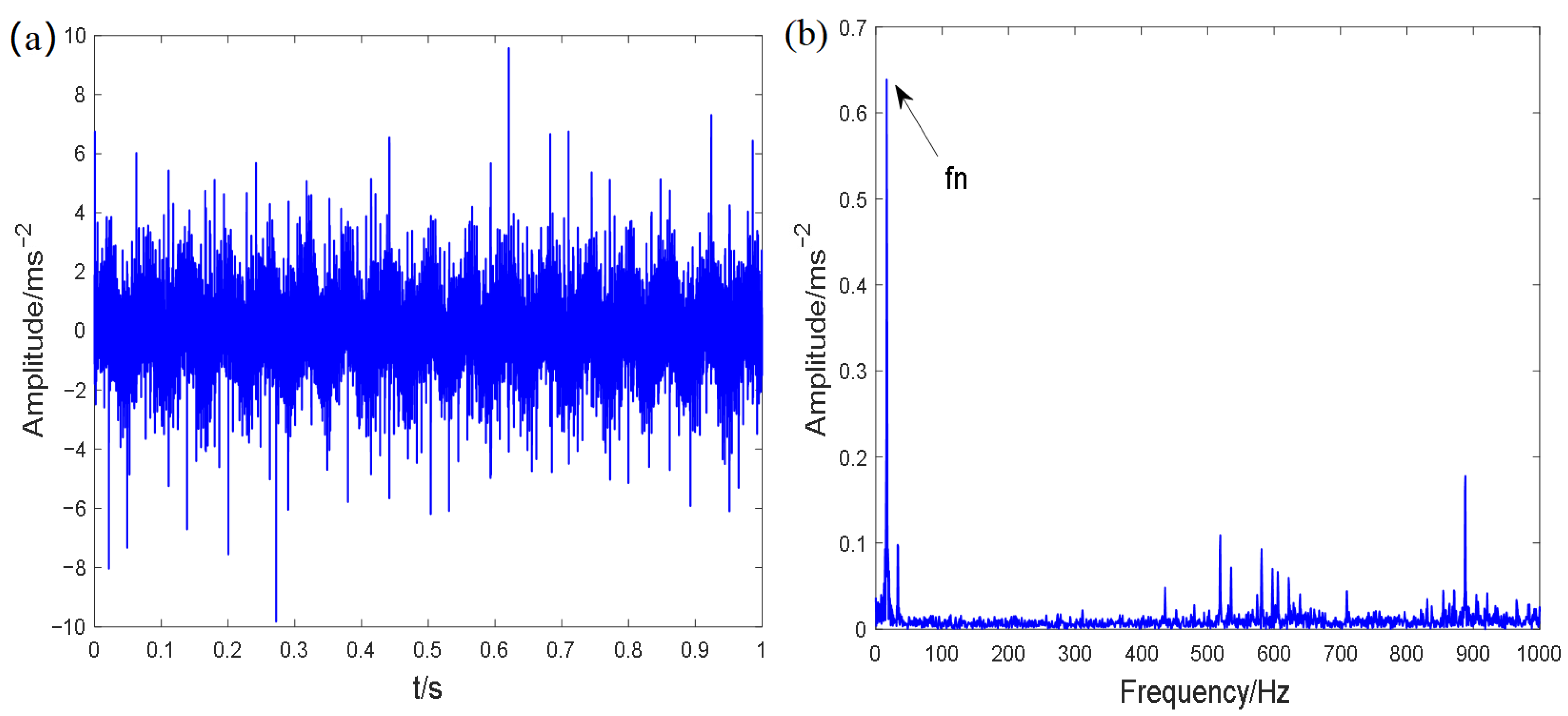
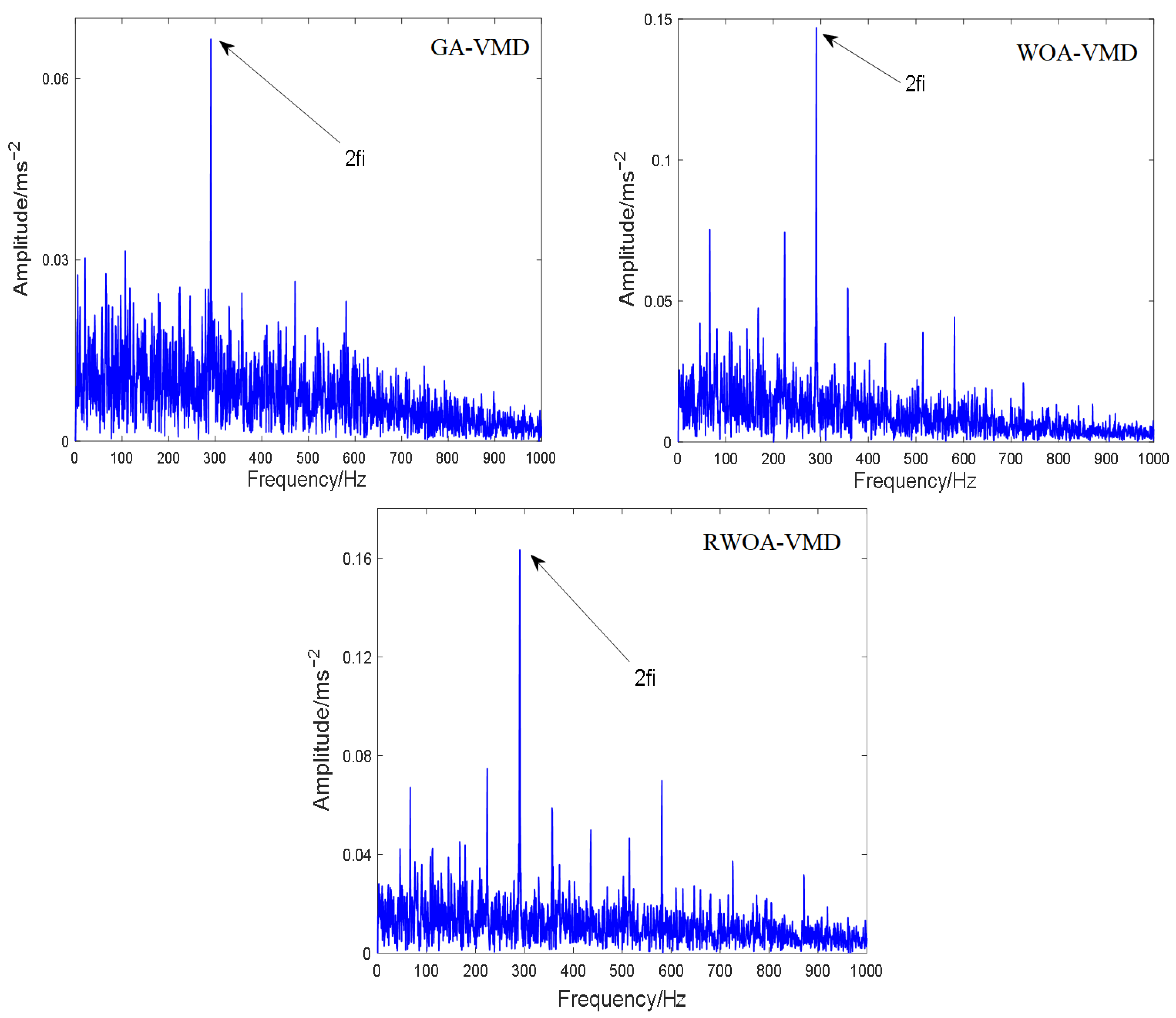
3.4. Experimental Validation of RWOA-VMD

In order to verify the effectiveness of RWOA-VMD, the vibration signal of the inner ring at the drive end is chosen from the Bearing Center of Case Western Reserve University (CWRU), the bearing speed is 1797 r/min, and the bearing inner ring fault frequency is $f_i=162.19$ Hz. To verify the advantages of the RWOA-VMD method in noise reduction and feature extraction, it is compared with GA-VMD and WOA-VMD. These three VMD optimization algorithms are set up to iterate 30 times with searching ranges of $K=\left[3,8\right]$ and $\alpha =\left[500,2000\right]$, and the final result takes the average of 30 tests. The minimum envelope entropy is set as the fitness function, and the adaptability optimization curve is shown in Figure 4. GA-VMD, WOA-VMD, RWOA-VMD run to the 19th, 18th, and 15th generation convergences, respectively, and the corresponding optimal parameter groups $\left[K,\alpha \right]$ are [5, 622], [5, 673], [4, 926].

Consequently, RWOA-VMD has the fastest convergence rate and the highest convergence precision. Each IMF1 of the three method has the minimum envelope entropy, respectively, 6.85, 6.84 and 6.81, and is selected for signal reconstruction. Figure 4 clearly verifies that envelope spectrum from RWOA-VMD has the most faults related to frequency components and the highest frequency amplitude. As a result, RWOA-VMD has prominent ability on fault feature enhancement.

4. A Novel Feature Enhancement Method for Vibrating Screen Exciter Bearing FAILURE

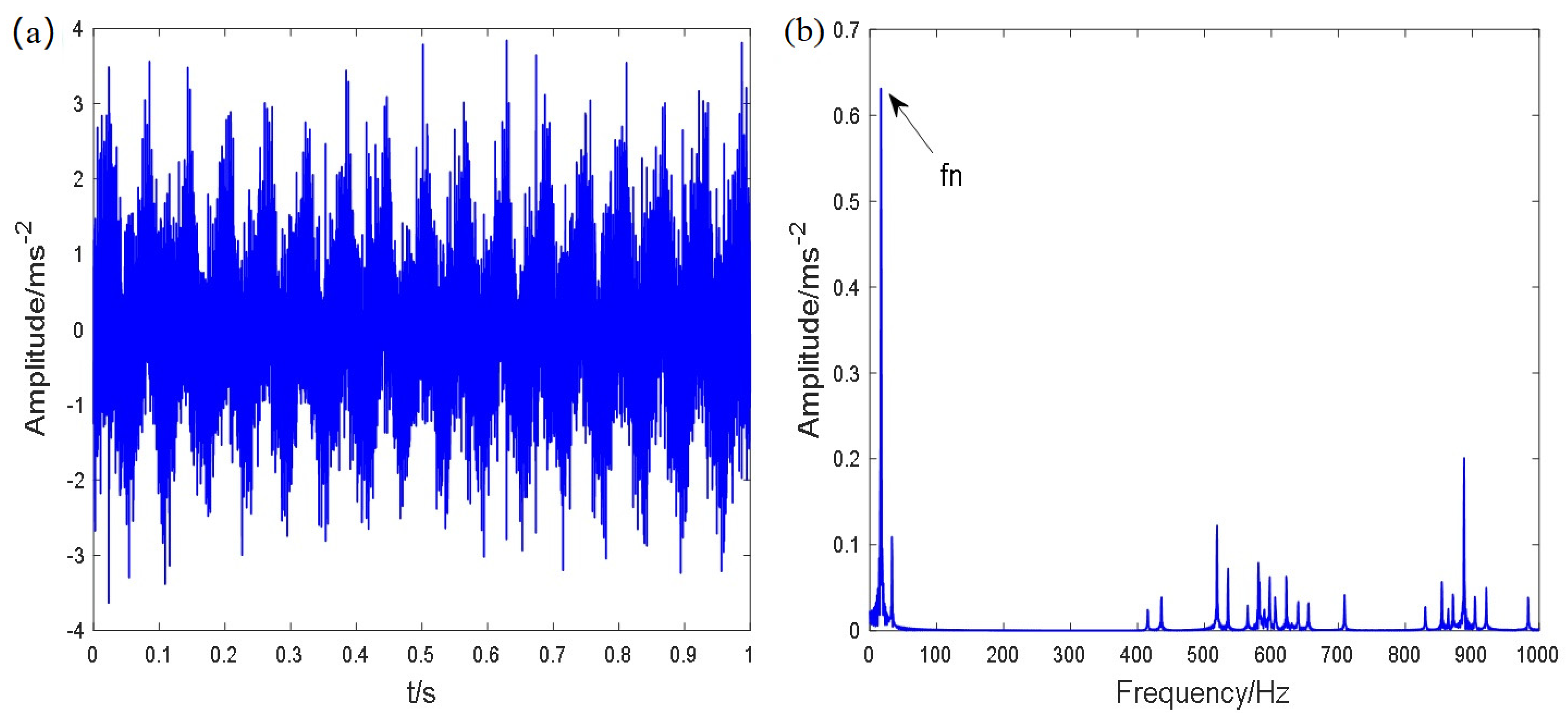
4.1. Experimental Arrangement

In Section 3.4, RWOA-VMD shows obvious advantages in bearing fault features extraction, but the test rig of CWRU simulates bearing faults on conventional rotating machinery, and in order to certify the application effect of RWOA-VMD in the context of vibrating machinery, e.g., vibrating screen exciter, the experimental verification is constructed. The relevant parameters of the tested bearing are shown in

Table 1. Bearing-related parameters.

Bearing Specification	Inner Diameter/mm	Outside Diameter/mm	Diameter/mm	Knot Diameter/mm	Number of Rollers	Contact Angle (°)
1308	40	90	12.5	65	15	30

and

Table 2. Fault bearing parameters.

Location	Width	Depth	Length	Length
Inner ring	1	0.2	Bearing width/2	Bearing width/2
Outer ring	0.7	0.2	Bearing width/2	Bearing width/2
Location	Rotation Speed/r/min	Rotation Frequency fn/Hz	Sampling FREQUENCY fs/Hz	Failure Frequency/Hz
Inner ring	910	15.17	20,000	104.92 (fo)
Outer ring	910	15.17	20,000	146.86 (fi)

.

The original vibration signal and frequency spectrum of the vibrating screen bearing with an inner ring fault are shown in Figure 5, which mainly presents the excitation frequency of the vibrating screen exciter because its energy is very large, and the early fault frequency is completely covered.

If GA-VMD, WOA-VMD and RWOA-VMD are, respectively, applied to the original signal, the results shown in Figure 6 only displays 2fi without other fault-related frequencies, e.g., harmonics and modulated frequencies. A conclusion is drawn that none of these three methods are remarkably effective in feature extraction of early fault of exciter bearing. It is necessary to propose a method which is more suitable for vibrating machinery.

4.2. Signal Processing Method Combining SSVD and RWOA-VMD

In order to enhance the fault characteristics of the bearing of vibrating screen exciter on the premise of reasonable noise reduction, this paper combines SSVD and RWOA-VMD for the processing of the original vibration signal. The overall procedure of this unified method is summarized in Figure 7 and the details are explained as follows:

Step 1: Noise pre-reduction SSVD is used to denoise the original vibration signal of exciter bearing with an inner race fault. Comparing Figure 8 and Figure 5, it can be found that noise is partly removed from the original signal, but the exciting frequency is still dominant and characteristic frequencies are still invisible.

Step 2: Fault features enhancement RWOA-VMD is used to decompose the denoised signal. After searching, the optimal parameter combination $\left[K,\alpha \right]$ is [4, 948]. As shown in Figure 9a, the signal after pre-denoising is decomposed into four levels, i.e., IMF1, IMF2, IMF3, and IMF4 at the first column with their frequency spectrums at the second column, and the last one is the residual component. Therefore, the first level obviously contains the exciting frequency of the vibrating screen and some relatively concentrated and orderly frequency components, that is, the envelope entropy is the minimum. By analogy, the envelope entropy of other layers increases in turn.

Step 3: Components screening and signal reconstruction. One or two components with the smallest envelop entropy are selected for signal reconstruction. IMF2 and IMF3 are chosen from Figure 9a to reconstruct the signal. By Hilbert transformation, the envelop spectrum of the reconstructed signal can obviously show the fault frequency and its harmonics.

Similarly, this method is used to process the vibration signal of the vibrating screen exciter with an outer race fault, as shown in Figure 9b. The result also displays a good effect of feature frequency extraction, which proves the universal applicability of this method.

In summary, the signal processing method based on the combination of SSVD and RWOA-VMD is verified to have a good application effect on the noise reduction and fault characteristic enhancement of vibration signals of the vibrating screen exciter bearing with early fault.

5. Early Fault Diagnosis Method of Vibrating Screen Exciter Bearing Based on AO-SVM Method

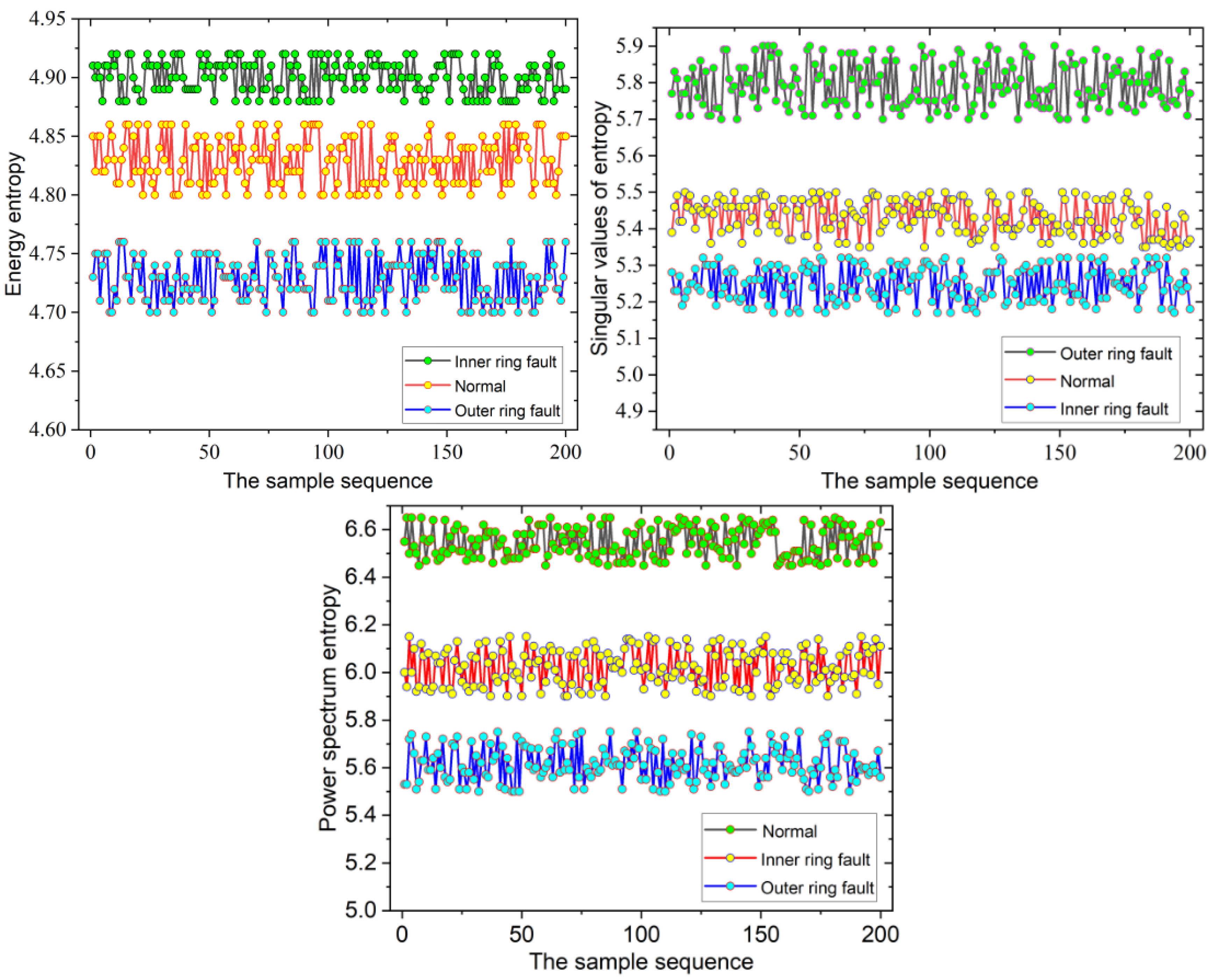
5.1. Fault Feature Extraction of Vibrating Screen Bearing

In order to identify and classify bearing faults, we construct a multi-mode feature matrix based on the energy entropy, singular value entropy, and power spectrum entropy calculated from signals processed by SSVD and RWOA-VMD, as shown in Figure 10. The energy entropy distribution is in different states, i.e., normal state, outer ring fault, and inner ring fault. A total of 200 sets of samples are adopted and each energy entropy is obtained from 1000 processed signals. The distribution of the energy entropy has good clustering and sensitivity. Similarly, the singular entropy distribution and power spectrum entropy distribution are exhibited in Figure 10. Therefore, due to good qualities, these three characteristic indexes can be used for fault diagnosis.

5.2. Support Vector Machine Optimized by Aquila Optimizer Algorithm (AO-SVM)

(1) Principle of AO algorithm

Inspired by the hunting behavior of aquila in nature, Laith A. [30] proposed an aquila optimizer algorithm (AO). As shown in Figure 11, the AO algorithm is divided into five steps:

① Initialization: Suppose N solutions are randomly generated from an initial population, and the predation space is D-dimensional. For D-dimensional, the optimization problem is:

$$\begin{gathered} minf\left(x\right) \\ s.t.UB\le x\le LB \end{gathered}$$

(20)

where $f\left(x\right)$ is the single objective optimization function, $X$ represents the set of current candidate solutions, as shown in Equation (21), which is randomly generated by Equation (18).

$$X=\left[\begin{array}{ccccc}{x}_{1,1}& \cdots & x_{1,j}& x_{1,D-1}& x_{1,D}\\ x_{2,1}& \cdots & x_{2,j}& \cdots & x_{2,D}\\ \cdots & \cdots & x_{i,j}& \cdots & \cdots \\ ⋮& ⋮& ⋮& ⋮& ⋮\\ x_{N-1,1}& \cdots & x_{N-1,j}& \cdots & x_{N-1,D}\\ x_{N,1}& \cdots & x_{N,j}& \cdots & x_{N,D}\end{array}\right]$$

(21)

$$x_{ij}=L{B}_j+rand\left(U{B}_j-L{B}_j\right),i=1,2,\dots ,Nj=1,2,\dots ,D$$

(22)

② Expanded Exploration $(X_1)$: During this step, the aquila recognizes the prey area and selects the best hunting area by high soar with vertical stoop. Figure 11a shows the high soar behavior with vertical stoop. The mathematical expression for this behavior is presented in Equation (23):

$$X_1\left(t+1\right)=X_{best}\left(t\right)\times \left(1-\frac{t}{T}\right)+\left(X_M\left(t\right)-X_{best}\left(t\right)\ast rand\right)$$

(23)

where $X_1\left(t+1\right)$ is the solution of the next iteration of $t$ generated by expansion exploration step $(X_1)$. $X_{best}\left(t\right)$ is the best solution obtained before the t-iteration, which reflects the approximate position of the prey, and $1-\frac{t}{T}$ is the expansion of the exploration by controlling the number of iterations. $X_M\left(t\right)$ represents the average of the current solution at the first t iteration, which is derived by Equation (24). $rand$ is a random number between 0 and 1. t and T represent the current iteration and the maximum number of iterations, respectively.

$$X_M\left(t\right)=\frac{1}{N}{\displaystyle \sum }_{i=1}^N{x}_i\left(t\right),\forall j=1,2,\dots ,D$$

(24)

③ Narrowed Exploration $(X_2)$: During this step, the aquila narrowly explores the selected area of the target prey in preparation for attacking. Figure 11b shows the short glide attack behavior of aquila’s contour flight, and the mathematical expression for this behavior is shown in Equation (25):

$$X_2\left(t+1\right)=X_{best}\left(t\right)\times Levy\left(D\right)+X_R\left(t\right)+\left(y-x\right)\ast rand)$$

(25)

where $X_2\left(t+1\right)$ is the solution of the next iteration of t generated by narrow exploration phase $(X_2)$. $X_{best}\left(t\right)$ is the best solution obtained before the tth iteration. $Levy\left(D\right)$ is Levy flight distribution function, derived from Equation (26), and $X_R\left(t\right)$ is the random solution obtained at the first iteration.

$$Levy\left(D\right)=s\times \frac{u\times \sigma }{{\left|v\right|}^{\frac{1}{\beta }}}$$

(26)

where s is a constant fixed to 0.01. u and v are random numbers between 0 and 1, and $\sigma$ derived from Equation (27).

$$\sigma =\left(\frac{\Gamma \left(1+\beta \right)\times \mathit{sin}e\left(\frac{\pi \beta }{2}\right)}{\Gamma \left(\frac{1+\beta }{2}\right)\times \beta \times 2^{\left(\frac{\beta -1}{2}\right)}}\right)$$

(27)

where $\beta$ is a constant value fixed to 1.5. In Equation (28), $y$ and $x$ are used to represent the spiral shape in the search, which are calculated as follows:

$$y=r\times \mathit{cos}\left(\theta \right)$$

(28)

$$x=r\times \mathit{sin}\left(\theta \right)$$

(29)

Thereinto:

$$r=r_1+U+D_1$$

(30)

$$\theta =-\omega \times D_1+{\theta }_1$$

(31)

$${\theta }_1=\frac{3\times \pi }{2}$$

(32)

where $r_1$ takes a value between 1 and 20 to represent the number of search periods, and U is a decimal number fixed to 0.00565. $D_1$ represents an integer between 1 and D. $\omega$ is a decimal number fixed to 0.005, and Figure 11c shows the spiral hunting behavior.

④ Expanded exploitation$(X_3)$: At this stage, the aquila narrows down to explore selected areas of the target prey in preparation for attack. Figure 11d shows the behavior of the aquila flying low with a slow descent attack, and the mathematical expression for this behavior is shown in Equation (33).

$$X_3\left(t+1\right)=(X_{best}\left(t\right)-X_M\left(t\right))\times \alpha -rand+\left(\left(UB-LB\right)\times rand+LB\right)\times \delta$$

(33)

where $X_3\left(t+1\right)$ is the solution for the next iteration of t generated by expanded exploitation $(X_3)$. $X_{best}\left(t\right)$ indicates the approximate position of the prey before the t-iteration (best solution obtained). $X_M\left(t\right)$ represents the average for the current solution at the t-iteration, which is derived from Equation (20). rand is a random value between 0 and 1. $\alpha$ and $\delta$ are development tuning parameters set between (0,1), and UB and LB represent the upper and lower limits of a given problem, respectively.

⑤ Narrowed Exploitation $(X_4)$: During this step, the aquila launches the ultimate attack on the prey in the last position. Figure 11e shows the behavior of the aquila in running and grabbing prey, and the mathematical expression for this behavior is shown in Equation (34).

$$\begin{gathered} X_4\left(t+1\right)=QF\times X_{best}\left(t\right)-\left(G_1\times X\left(t\right)\times rand\right) \\ -G_2\times Levy\left(D\right)+rand\times G_1 \end{gathered}$$

(34)

where $X_4\left(t+1\right)$ is the solution of the next iteration of $t$ generated by the narrowed exploitation $(X_4)$. QF represents the mass function used to balance the search strategy, derived from Equation (35); $G_1$ represents the random flight posture of the Sky hawk tracking prey during the run, derived from Equation (36); $G_2$ presents a regressive impairment from 2 to 0 to indicate the flight slope of the Sky hawk running from the first position (1) to the last position (t), derived from Equation (37). $X\left(t\right)$ is the current solution of the t iteration.

$$QF\left(t\right)=t^{\frac{2\times rand-1}{{\left(1-T\right)}^2}}$$

(35)

$$G_1=2\times rand-1$$

(36)

$$G_2=2\times \left(1-\frac{t}{T}\right)$$

(37)

$QF\left(t\right)$ is the mass function value at the time of the tth iteration. rand is a random value between 0 and 1, and t and T indicate the current number of iterations and the maximum number of iterations, respectively. $Levy\left(D\right)$ is derived from Equation (26) of levy’s flight distribution function, and Figure 11f shows the effect of the quality function (QF), G₁, and G₂ on AO’s behavior.

(2) SVM process optimized by AO algorithm

When the AO algorithm explores the approximate optimal solution or the reasonable position of the optimal solution of a set of random candidate solutions through search strategies, in order to emphasize the balance between AO search strategies (i.e., exploration and exploitation), exploration and exploration set up different search strategies (i.e., expanded exploration, narrowed exploration, expanded exploitation, and narrowed exploitation). The process of optimizing the SVM is shown in Figure 12.

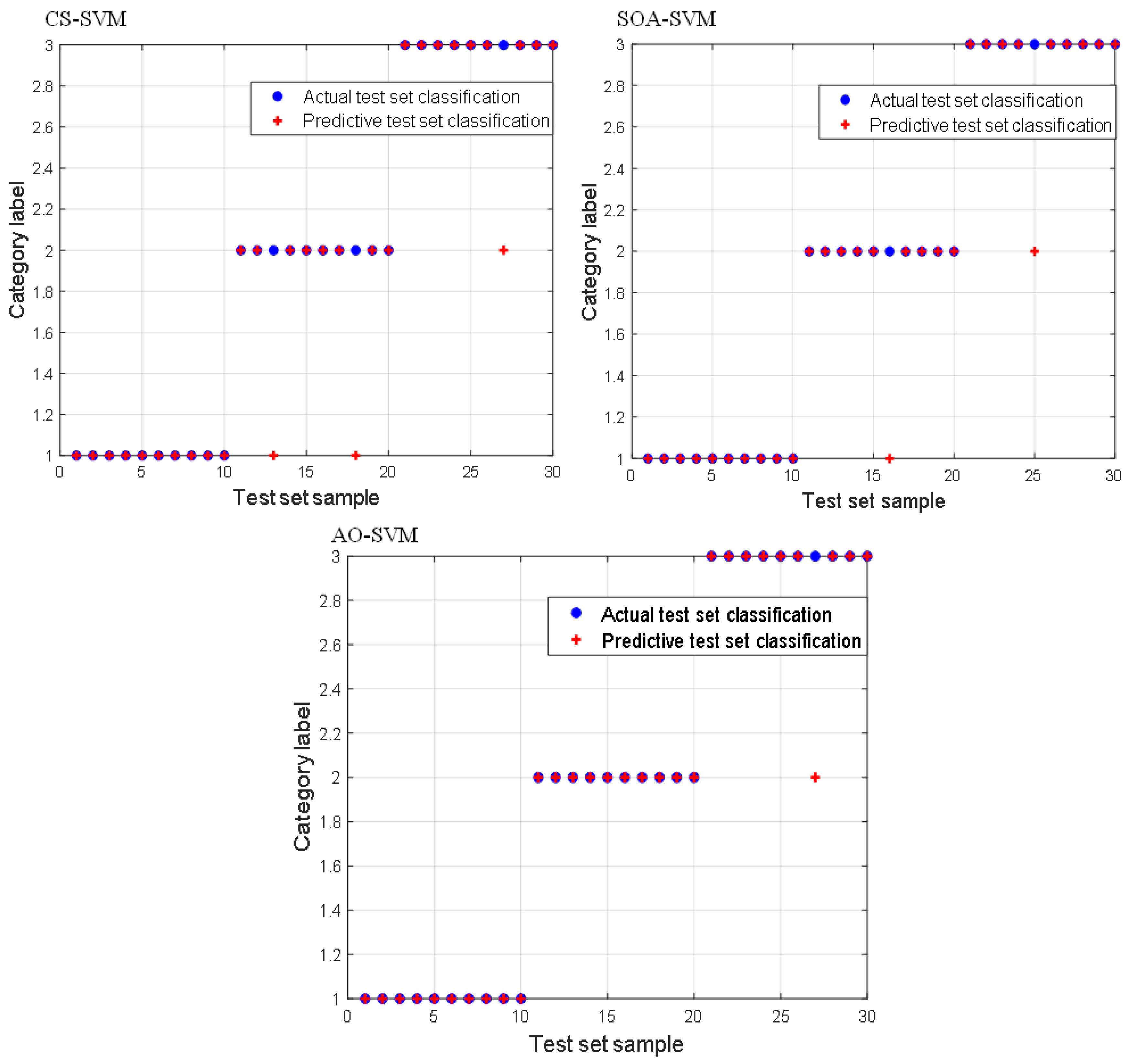
5.3. Application Comparison of Different SVM Optimization Algorithms

In order to verify that the AO-SVM-based algorithm has a better fault diagnosis capability, the optimized SVM based on the seagull optimization algorithm (SOA) and the optimized SVM based on the cuckoo search (CS) are selected for comparison.

Multi-modal features are, respectively, calculated and input to the AO-SVM, SOA-SVM, CS-SVM models. The kernel function width g affects the learning performance of SVM. When g is too large, the sample data cannot be effectively distinguished by the SVM classifier; although the sample data can be correctly classified when g is too small, the algorithm is very easy to over fit, resulting in the unknown samples cannot be correctly classified. The penalty factor C is another important parameter. When C is large, the generalization ability of SVM will be reduced; when C is small, the sample data cannot be fully trained by the SVM model, and the risk of inadequate learning and fitting error increase. Based on the above considerations, the optimization range of SVM penalty parameter C is [0.01, 100]; and the optimization range of the width of the kernel function g is [0.01, 100]. Moreover, the population parameters of the three models are set to 20; the maximum number of iterations is 50 times. There are 50 sets of data for each state as training groups and 10 sets of data for each state as test groups. The comparison of recognition results of CS-SVM, SOA-SVM, and AO-SVM is shown in Figure 13.

Table 3. Comparison of SVM optimization algorithms.

SVM Model	Penalty Parameters C	Kernel Function Width g	Accuracy (%)
CS-SVM	76.9775	56.3112	90.0000
SOA-SVM	61.4716	98.3154	93.3333
AO-SVM	46.2141	22.6567	96.6667

demonstrates that AO-SVM has the highest accuracy for fault diagnosis. Therefore, a conclusion is drawn that the multi-modal features and AO-SVM algorithm proposed in Section 5.1 and Section 5.3 has a good application effect in the early fault diagnosis of vibrating screen bearing.

6. Conclusions

In this paper, taking the vibrating screen from vibrating machinery as an example, the extraction of early fault characteristics and fault diagnosis methods of the bearing of vibrating screen exciter are studied. Based on the study, the conclusions and novelties of this paper can be drawn:

• Considering the strong background noise of the early fault signal of bearings, an improved SVD based on singular value’s unilateral ascent method, i.e., SSVD, for pre-denoising is proposed.
• In view of the weak fault characteristics of the early fault signal of bearings, a fault feature enhancement method, i.e., variational modal decomposition improved by revised whale algorithm optimization (RWOA-VMD), is proposed.
• Considering that the early fault characteristics of the vibrating screen bearings are much weaker than those of the traditional rotating machinery, it is impossible to effectively extract fault features by separately using SSVD or RWOA-VMD; and then, the joint application of SSVD and RWOA-VMD can achieve remarkable application effects.
• In order to intelligently realize the early fault diagnosis of the bearing of vibrating screen bearings, a multi-modal feature matrix consisting of the energy entropy, singular value entropy, and power spectrum entropy, is constructed.
• By improving the support vector machine using the Aquila optimizer algorithm, the early fault diagnosis of vibrating screen bearings is accurately realized.

As described in the paper, it requires the combination of SSVD and RWOA-VMD methods, which means that the time spent is a little longer. Therefore, further study is needed to improve the efficiency of the method. Moreover, the experiment is only conducted for the single point corrosion of the inner and outer rings of the vibrating screen bearing, so it is necessary to continue to verify the effectiveness of this method for coupling failures such as multiple point corrosion of the bearing components.

References

1. Lv, G. Present Situation and Development Trend of Vibrating Screen Equipment. Coal Min. Mach. 2021, 42, 41–43. [Google Scholar]
2. Vashisht, R.; Peng, Q. Crack detection in the rotor ball bearing system using switching control strategy and Short Time Fourier Transform. J. Sound Vib. 2018, 432, 502–529. [Google Scholar] [CrossRef]
3. Li, J.; Yao, X.; Wang, H.; Zhang, J. Periodic impulses extraction based on improved adaptive VMD and sparse code shrinkage denoising and its application in rotating machinery fault diagnosis. Mech. Syst. Signal Process. 2019, 126, 568–589. [Google Scholar] [CrossRef]
4. Lei, Y.; Lin, J.; He, Z.; Zuo, M. A review on empirical mode decomposition in fault diagnosis of rotating machinery. Mech. Syst. Signal Process. 2013, 35, 108–126. [Google Scholar] [CrossRef]
5. Wu, Z.; Huang, N. Ensemble empirical mode decomposition: A noise-assisted data analysis method. Adv. Adapt. Data Anal. 2009, 1, 1–41. [Google Scholar] [CrossRef]
6. Gilles, J. Empirical wavelet transform. IEEE Trans. Signal Process. 2013, 61, 3999–4010. [Google Scholar] [CrossRef]
7. Dragomiretskiy, K.; Zosso, D. Variational mode decomposition. IEEE Trans. Signal Process. 2014, 62, 531–544. [Google Scholar] [CrossRef]
8. Zheng, J.; Cheng, J.; Yang, Y. Modified EEMD algorithm and its applications. J. Vib. Shock 2013, 32, 21–26+46. [Google Scholar]
9. Kedadouche, M.; Thomas, M.; Tahan, A. A comparative study between Empirical Wavelet Transforms and Empirical Mode Decomposition Methods: Application to bearing defect diagnosis. Mech. Syst. Signal Process. 2016, 11, 88–107. [Google Scholar] [CrossRef]
10. Li, Q.; Liao, X.; Zhang, Q.; Cui, D. Feature Extraction and Classification of Bearings Based on EWT and Multi-Scale Entropy. Bearing 2016, 1, 48–52. [Google Scholar]
11. Chen, J.; Pan, J.; Li, Z.; Zi, Y.; Chen, X. Generator bearing fault diagnosis for wind turbine via empirical wavelet transform using measured vibration signals. Renew. Energy 2016, 89, 80–92. [Google Scholar] [CrossRef]
12. Yan, B.; Nie, S.; Tang, B.; Liu, Z. Research on Bearing Fault Diagnosis Based on Order Analysis and EWT. Modul. Mach. Tool Autom. Manuf. Tech. 2018, 7, 51–54. [Google Scholar]
13. Zhu, W.; Feng, Z. Fault diagnosis of planetary gearbox based on improved empirical wavelet transform. Chin. J. Sci. Instrum. 2016, 37, 2193–2201. [Google Scholar]
14. Amezquitasanchez, J.; Adeli, H. A new music-empirical wavelet transform methodology for time-frequency analysis of noisy nonlinear and non-stationary signals. Digit. Signal Process. 2015, 45, 55–68. [Google Scholar] [CrossRef]
15. Wang, D.; Tsui, K.; Qin, Y. Optimization of segmentation fragments in empirical wavelet transform and its applications to extracting industrial bearing fault features. Measurement 2019, 133, 328–340. [Google Scholar] [CrossRef]
16. Jiang, F.; Zhu, Z.; Li, W. An improved VMD with empirical mode decomposition and its application in incipient fault detection of rolling bearing. IEEE Access 2016, 6, 44483–44493. [Google Scholar] [CrossRef]
17. Shi, P.; Yang, W. Precise feature extraction from wind turbine condition monitoring signals by using optimised variational mode decomposition. Renew. Power Gener. IET 2017, 11, 245–252. [Google Scholar] [CrossRef] [Green Version]
18. Zhu, J.; Wang, C.; Hu, Z.; Kong, F. Adaptive variational mode decomposition based on artificial fish swarm algorithm for fault diagnosis of rolling bearings. Proc. Inst. Mech. Eng. Part C J. Mech. Eng. Sci. 2017, 231, 45–52. [Google Scholar] [CrossRef]
19. Wang, X.; Yang, Z.; Yan, X. Novel particle swarm optimization-based variational mode decomposition method for the fault diagnosis of complex rotating machinery. IEEE-ASME Trans. Mechatron. 2017, 23, 68–79. [Google Scholar] [CrossRef]
20. Wang, Z.; He, G.; Du, W.; Zhou, J.; Han, X.; Wang, J.; He, H.; Guo, X.; Wang, J.; Kou, Y. Application of parameter optimized variational mode decomposition method in fault diagnosis of gearbox. IEEE Access 2019, 7, 44871–44882. [Google Scholar] [CrossRef]
21. Cheng, C.; Wang, W.; Chen, H.; Zhang, B.; Shao, J.; Teng, W. Enhanced fault diagnosis using broad learning for traction systems in high-speed trains. IEEE Trans. Power Electron. 2021, 36, 7461–7469. [Google Scholar] [CrossRef]
22. Chen, H.; Jiang, B. A review of fault detection and diagnosis for the traction system in high-speed trains. IEEE Trans. Intell. Transp. Syst. 2020, 21, 450–465. [Google Scholar] [CrossRef]
23. Chen, H.; Jiang, B.; Ding, S.; Huang, B. Data-driven fault diagnosis for traction systems in high-speed trains: A survey, challenges, and perspectives. IEEE Trans. Intell. Transp. Syst. 2020, 23, 1700–1716. [Google Scholar] [CrossRef]
24. Chen, H.; Jiang, B.; Lu, N. A multi-mode incipient sensor fault detection and diagnosis method for electrical traction systems. Int. J. Control Autom. Syst. 2018, 16, 1783–1793. [Google Scholar] [CrossRef]
25. Chen, H.; Jiang, B.; Zhang, T.; Lu, N. Data-driven and deep learning-based detection and diagnosis of incipient faults with application to electrical traction systems. Neurocomputing 2020, 396, 429–437. [Google Scholar] [CrossRef]
26. Xu, Y.; Cai, Z. Application of Variational Modal Decomposition and K-L Divergence to Bearing Fault Diagnosis of Vibrating Screens. Noise Vib. Control 2017, 36, 306–308. [Google Scholar]
27. Cai, Z.; Xu, Y.; Duan, Z. An alternative demodulation method using envelope-derivative operator for bearing fault diagnosis of the vibrating screen. J. Vib. Control JVC 2018, 24, 3249–3261. [Google Scholar] [CrossRef]
28. Li, Z.; Zhang, W.; Ming, A.; Li, Z.; Chu, F. A Novel Fault Diagnosis Method Based on Improved Empirical Wavelet Transform and Maximum Correlated Kurtosis Deconvolution for Rolling Element Bearing. J. Mech. Eng. 2019, 55, 136–146. [Google Scholar]
29. Mirjalili, S.; Lewis, A. The Whale Optimization Algorithm. Adv. Eng. Softw. 2016, 95, 51–67. [Google Scholar] [CrossRef]
30. Abualigah, L.; Yousri, D.; Elaziz, M.A.; Ewees, A.A.; Al-qaness, M.A.A.; Gandomi, A.H. Aquila Optimizer: A novel meta-heuristic optimization algorithm. Comput. Ind. Eng. 2021, 157, 1–59. [Google Scholar] [CrossRef]
31. Abualigah, L. Aquila Optimizer: A meta-heuristic optimization algorithm, MATLAB Central File Exchange. Retrieved 1 November 2022. Available online: https://www.mathworks.com/matlabcentral/fileexchange/89386-aquila-optimizer-a-meta-heuristic-optimization-algorithm (accessed on 1 June 2022).
Figure 1. Comparison of frequency spectrums: (a) without noise and (b) with noise (SNR = 1).
Machines 10 01007 g001
Figure 2. (a) noise reduction based on SSVD and (b) based on singular value difference spectra.
Machines 10 01007 g002
Figure 3. Flowchart of RWOA-VMD.
Machines 10 01007 g003
Figure 4. Comparison of processing effect based on GA-VMD, WOA-VMD and RWOA-VMDA.
Machines 10 01007 g004
Figure 5. (a) original vibration signal and (b) frequency spectrum of vibrating screen bearing with inner ring fault.
Machines 10 01007 g005
Figure 6. Comparison of processing effect directly using: GA-VMD, WOA-VMD and RWOA-VMD in the condition of exciter bearing with inner ring fault.
Machines 10 01007 g006
Figure 7. The flow chart of the method of combining SSVD and RWOA-VMD for signal processing of vibrating screen exciter bearing.
Machines 10 01007 g007
Figure 8. (a) signal pre-denoising by SSVD with inner ring fault and (b) frequency spectrum.
Machines 10 01007 g008
Figure 9. The application effect of RWOA-VMD on the vibration signals of vibrating screen exciter: (a) inner ring fault and (b) outer ring fault.
Machines 10 01007 g009
Figure 10. Distributions of energy entropy, singular value entropy, and power spectral entropy in different conditions.
Machines 10 01007 g010
Figure 11. The influence of the principles and parameters of each step of the aquila optimizer algorithm on AO: (a) expanded exploration; (b) narrowed exploration; (c) expanded exploitation; (d) narrowed exploitation; (e) narrowed exploitation; (f) the effects of the quality function (QF), G1 and G2 on the behavior of the AO [30,31].
Machines 10 01007 g011
Figure 12. The flowchart of SVM improved by AO algorithm.
Machines 10 01007 g012
Figure 13. Comparison of identification results of three SVM algorithms: CS-SVM, SOA-SVM, and AO-SVM.
Machines 10 01007 g013