
Evaluation System of Curved Conveyor Belt Deviation State Based on the ARIMA–LSTM Combined Prediction Model

Abstract
:1. Introduction
2. Construction of Conveyor Belt Deviation Experimental System
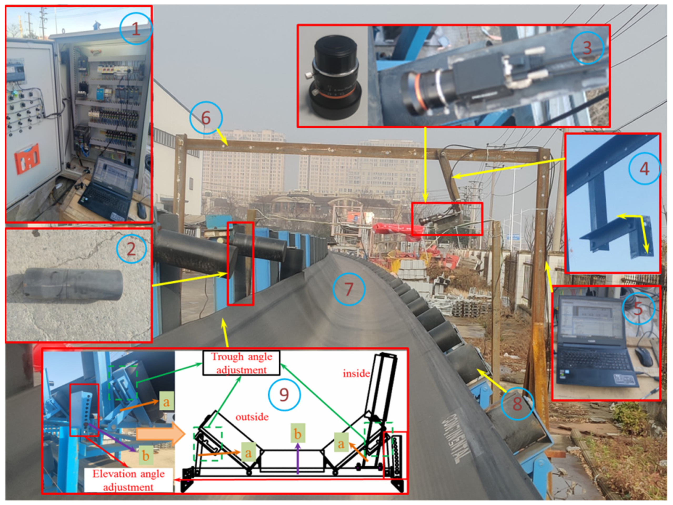
2.1. Conveyor Belt Deviation Measurement Test Bed
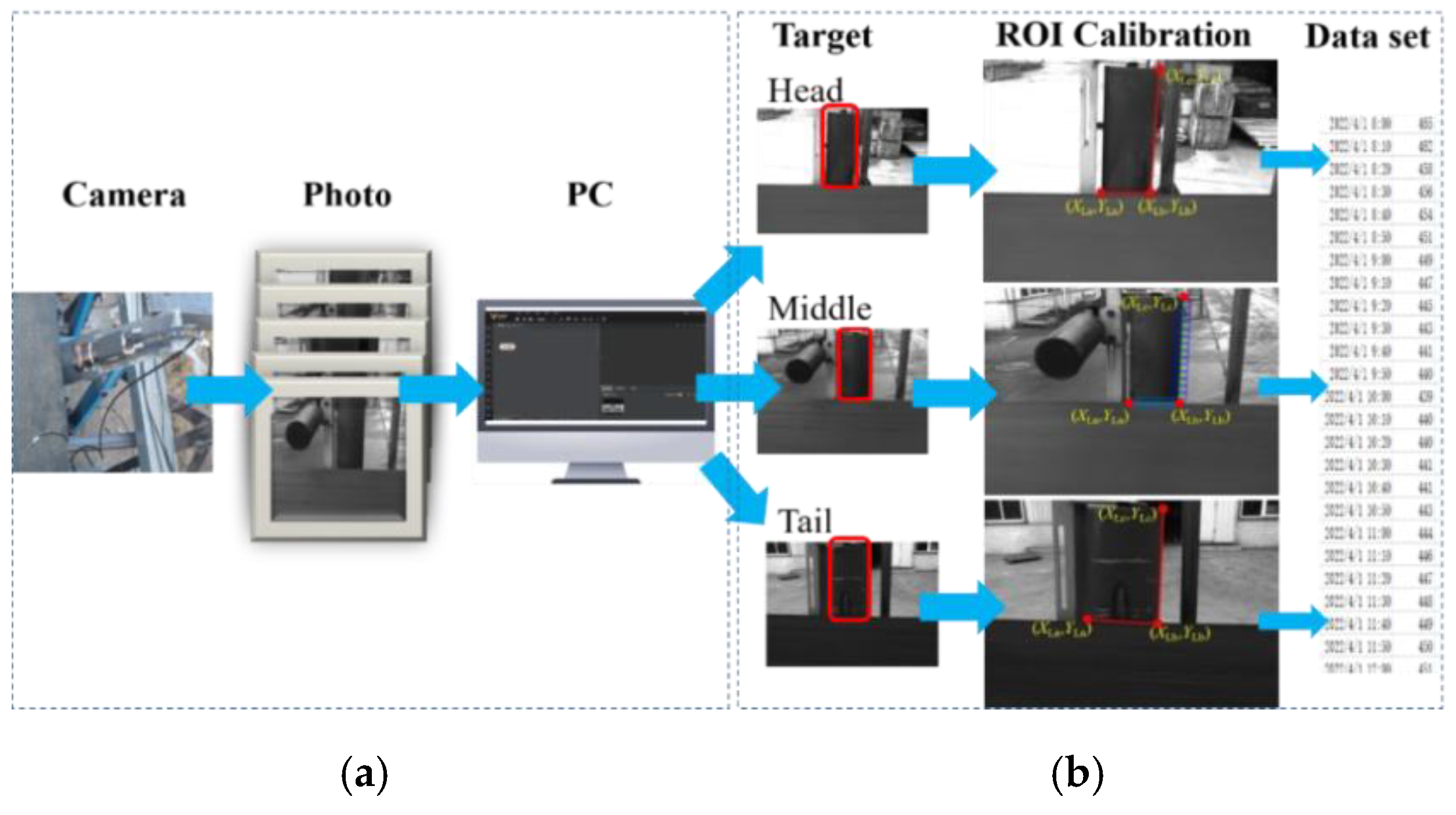
2.2. Deviation Data Acquisition
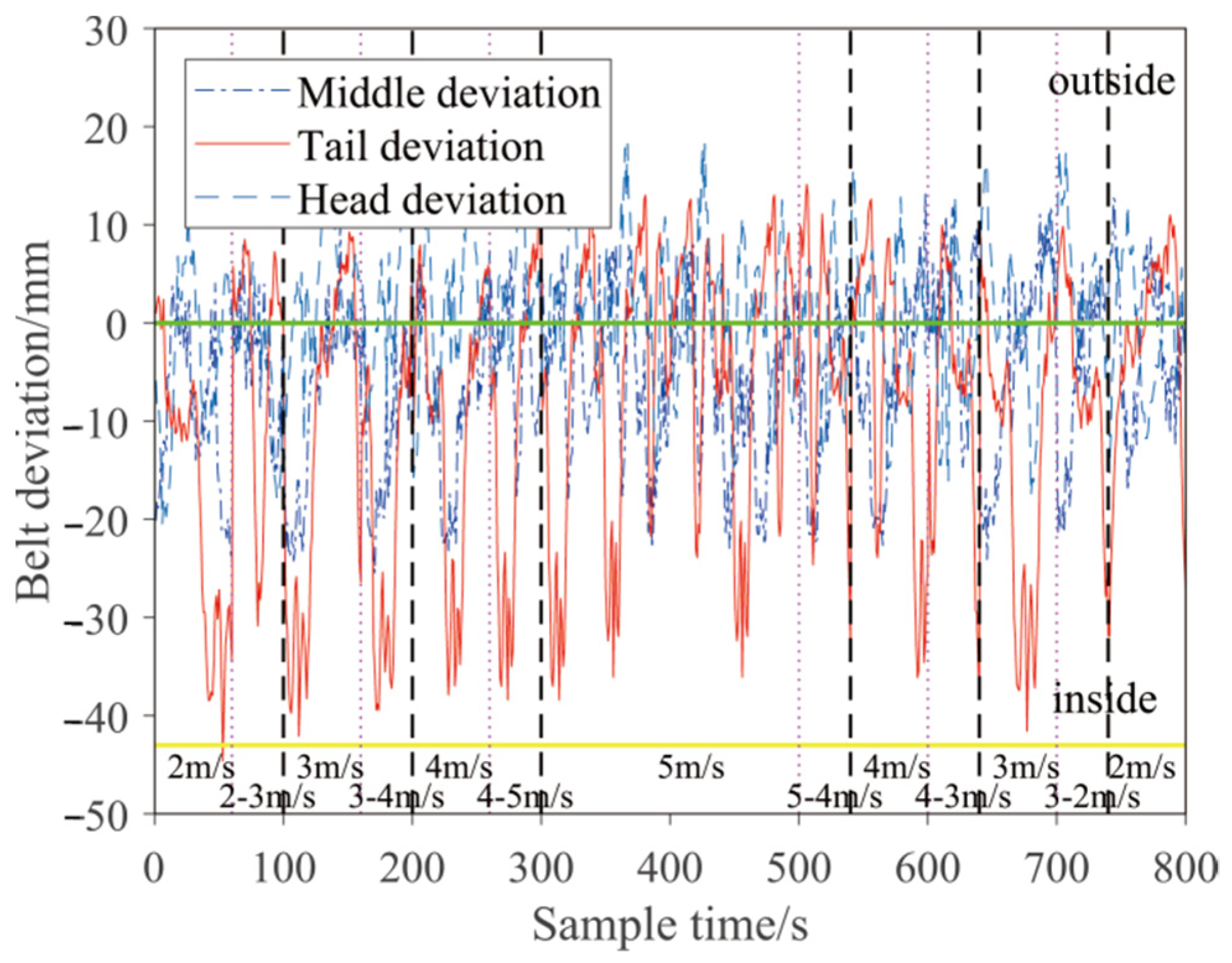
2.3. Determination of Deviation Detection Position
3. Establishment of Mechanical Model of Conveyor Belt Deviation in the Curve Section
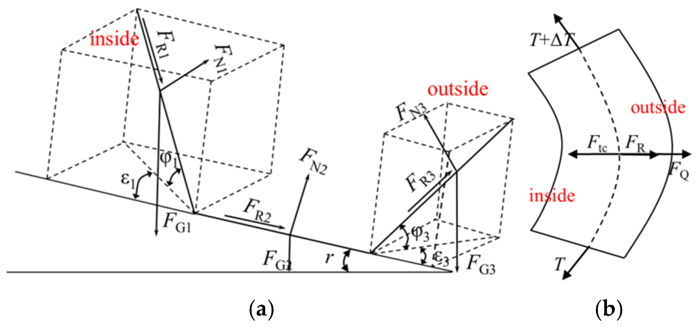
3.1. Force Equilibrium Equation
3.2. Material and Conveyor Belt Gravity Distribution Coefficient
3.3. Model Validation
3.4. Correction Deviation Range of Idler Frame Angle
4. Establishment of the Prediction Model of Conveyor Belt Deviation
4.1. ARIMA Prediction Model
4.2. LSTM Prediction Model
4.3. ARIMA–LSTM Combined Prediction Model Based on Series–Parallel Weighting
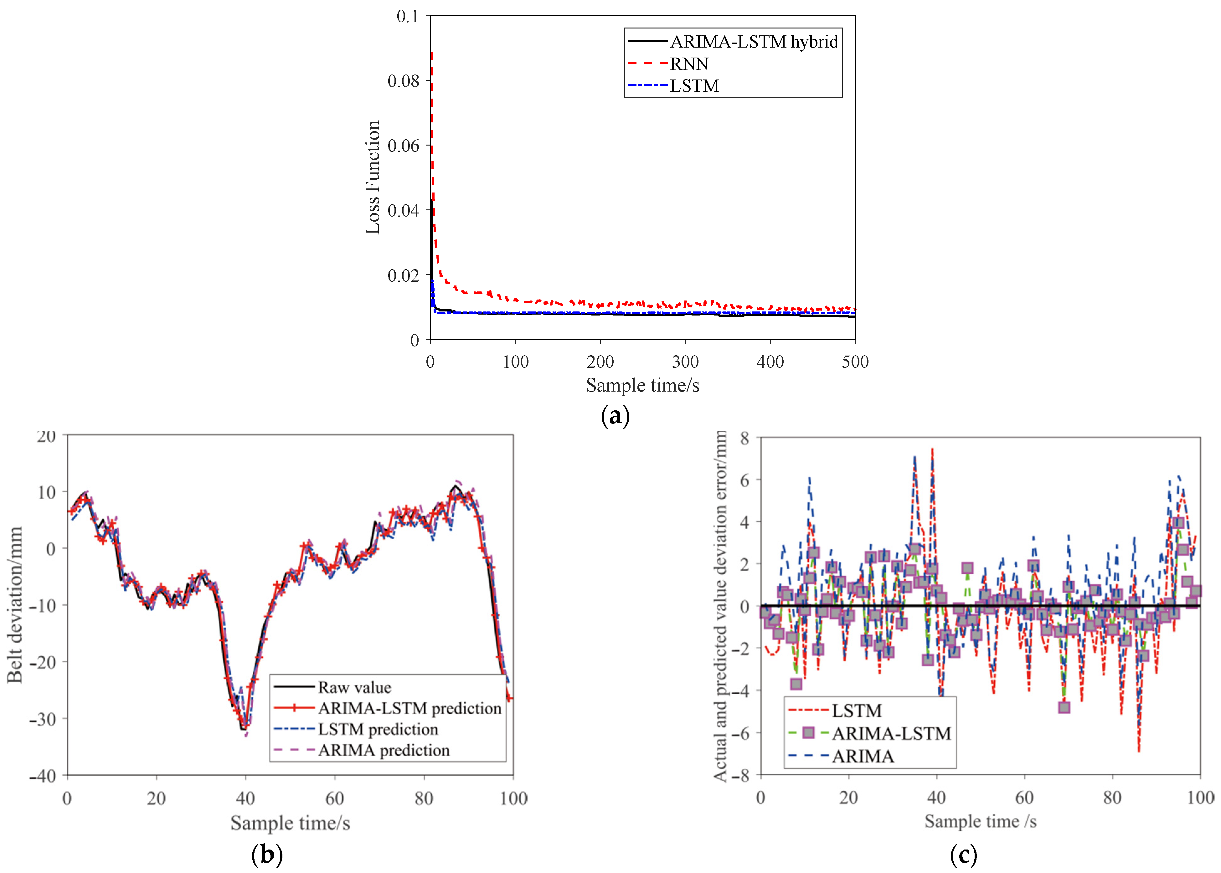
4.4. Comparison of Fitting Degree of Different Prediction Models
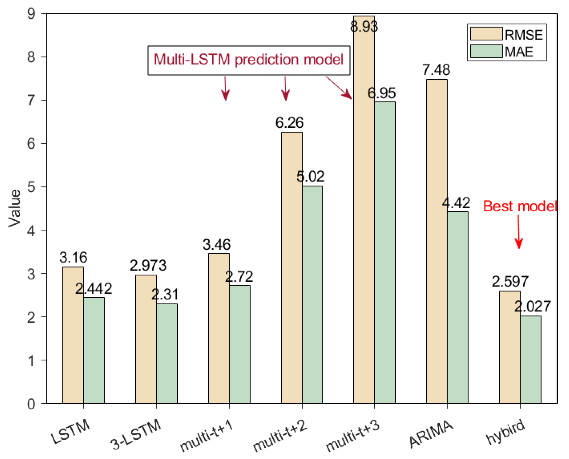
4.5. Performance Comparison of Different Prediction Models
5. Establishment of Conveyor Belt Condition Evaluation System
5.1. Application of the Prediction Model in the Correctable Deviation Range
5.2. Anomaly Detection of Conveyor Belt Deviation Based on OCSVM
5.3. Establishment of Visual Interactive Interface
5.4. Experimental Verification
6. Conclusions
Author Contributions
Funding
Institutional Review Board Statement
Informed Consent Statement
Data Availability Statement
Conflicts of Interest
References
- Grimmer, K.-J.; Kessler, F. The design of belt conveyors with horizontal curves. Bulk Solids Handl. J. 1992, 12, 557–563. [Google Scholar]
- Kessler, F.; Grabner, K.; Grimmer, K.-J. “bico-Tec” A new type of belt conveyor with horizontal curve. Bulk Solids Handl. J. 1993, 13, 741–747. [Google Scholar]
- Leberwirth, H. Design of belt conveyors with horizontal curves. Bulk Solids Handl. J. 1994, 14, 283–285. [Google Scholar]
- Tooker, G.E. Suspension idler is used in the horizontal curves. Bulk Solids Handl. J. 1988, 8. [Google Scholar]
- Cheng, X.; Du, H. Resistance Analysis of Belt Conveyor during Horizontal Turning Section. Adv. Mater. Res. 2011, 201–203, 467–470. [Google Scholar] [CrossRef]
- Zhao, L.; Lin, Y. Typical failure analysis and processing of belt conveyor. J. Procedia Eng. 2011, 26, 942–946. [Google Scholar] [CrossRef]
- Gupta, A. Analysis for Controlling Belt Deviation in Conveyor System. Am. J. Comput. Sci. Eng. Surv. 2013, 1, 53–58. [Google Scholar]
- Zhao, Y.; Li, Y. The present and future development of belt conveyer. J. Coal Mine Mach. 2004, 4, 1–3. [Google Scholar] [CrossRef]
- Wang, T.; Dong, Z.; Liu, J. Research of mine conveyor belt deviation detection system based on machine vision. J. Min. Sci. 2021, 57, 703–712. [Google Scholar] [CrossRef]
- Liu, Y.; Miao, C.; Li, X.; Xu, G. Research on Deviation Detection of Belt Conveyor Based on Inspection Robot and Deep Learning. Complexity 2021, 2021, 3734560. [Google Scholar] [CrossRef]
- Yang, Y.; Miao, C.; Li, X.; Mei, X. On-line conveyor belts inspection based on machine vision. Optik 2014, 125, 5803–5807. [Google Scholar] [CrossRef]
- Yang, Y.L.; Miao, C.Y.; Kang, K.; Li, X. Machine vision inspection technique for conveyor belt deviation. J. North Univ. China Nat. Sci. Ed. 2012, 33, 667–671. [Google Scholar]
- Wang, J.; Liu, Q.; Dai, M. Belt vision localization algorithm based on machine vision and belt conveyor deviation detection. In Proceedings of the 2019 34rd Youth Academic Annual Conference of Chinese Association of Automation (YAC), Jinzhou, China, 6–8 June 2019; IEEE: Piscataway, NJ, USA, 2019; pp. 269–273. [Google Scholar] [CrossRef]
- Zhang, M.; Shi, H.; Yu, Y.; Zhou, M. A computer vision based conveyor deviation detection system. J. Appl. Sci. 2020, 10, 2402. [Google Scholar] [CrossRef] [Green Version]
- Liu, Y.; Wang, Y.; Zeng, C.; Zhang, W.; Li, J. Edge Detection for Conveyor Belt Based on the Deep Convolutional Network. In Proceedings of the 2018 Chinese Intelligent Systems Conference, Wenzhou, China, 17–22 November 2018; Lecture Notes in Electrical Engineering. Jia, Y., Du, J., Zhang, W., Eds.; Springer: Singapore, 2019; Volume 529. [Google Scholar] [CrossRef]
- Zhang, M.; Jiang, K.; Cao, Y.; Li, M.; Hao, N.; Zhang, Y. A deep learning-based method for deviation status detection in intelligent conveyor belt system. J. Clean. Prod. 2022, 363, 132575. [Google Scholar] [CrossRef]
- Kirjanów-Błażej, A.; Jurdziak, L.; Burduk, R.; Błażej, R. Forecast of the remaining lifetime of steel cord conveyor belts based on regression methods in damage analysis identified by subsequent DiagBelt scans. Eng. Fail. Anal. 2019, 100, 119–126. [Google Scholar] [CrossRef]
- Hu, X.; Zong, M. Fault Prediction Method of Belt Conveyor Based on Grey Least Square Support Vector Machine. In Proceedings of the International Conference on Measuring Technology and Mechatronics Automation (ICMTMA), Beihai, China, 16–17 January 2021; pp. 55–58. [Google Scholar]
- Liu, X.; He, D.; Lodewijks, G.; Pang, Y.; Mei, J. Integrated decision making for predictive maintenance of belt conveyor systems. Reliab. Eng. Syst. Saf. 2019, 188, 347–351. [Google Scholar] [CrossRef]
- Mei, X.; Miao, C.; Yang, Y.; Li, X. Rapid inspection technique for conveyor belt deviation. J. Mech. Eng. Res. Dev. 2016, 39, 653–662. [Google Scholar]
- Wang, D.; Song, W.; Liu, J. Dynamic Design and Computer Imitation of Belt Conveyor with Horizontal Curves. Adv. Eng. Forum 2011, 2–3, 833–837. [Google Scholar]
- Bing, L. The Design and Application of Long Distance Belt Conveyor with Horizontal Curves. Master’s Thesis, Dalian University of Technology, Dalian, China, 2013. [Google Scholar]
- Wang, H.; Xv, L.; Qiu, Y.; Xiang, Y.; Hu, S. Design of turning radius of long distance belt conveyor of Changjiu Limestone Mine. Opencast Min. Technol. 2019, 34, 97–100. [Google Scholar]
- Wang, H. Study of Design Technology for Long Distance Horizontal Curve Belt Conveyor. Master’s Thesis, Dalian University of Technology, Dalian, China, 2013. [Google Scholar]
- Yang, L. Research on Design and Calculation Theory of Belt Conveyor with Horizontal Curves. Master’s Thesis, Northeastern University, Shenyang, China, 2014. [Google Scholar]
- Tian, L. Research on Key Technologies of Long Distance Horizontal Turning Belt Conveyor. Master’s Thesis, Taiyuan University of Science and Technology, Taiyuan, China, 2012. [Google Scholar]
- Hong, T.; Fan, S. Probabilistic electric load forecasting: A tutorial review. Int. J. Forecast. 2016, 32, 914–938. [Google Scholar] [CrossRef]
- Wang, X.; Wu, J.; Liu, C.; Yang, H.; Du Yanli, N.I. Exploring LSTM based recurrent neural network for failure time series prediction. J. Beijing Univ. Aeronaut. Astronaut. 2018, 44, 772–784. [Google Scholar] [CrossRef]
- Ning, Y.; Kazemi, H.; Tahmasebi, P. A comparative machine learning study for time series oil production forecasting: ARIMA, LSTM, and Prophet. Comput. Geosci. 2022, 164, 105126. [Google Scholar] [CrossRef]
- Shi, H.; Xu, M.; Li, R. Deep learning for household load forecasting—A novel pooling deep RNN. IEEE Trans. Smart Grid 2018, 9, 5271–5280. [Google Scholar] [CrossRef]
- Willmott, C.; Matsuura, K. Advantages of the mean absolute error (MAE) over the root mean square error (RMSE) in assessing average model performance. Clim. Res. 2005, 30, 79. [Google Scholar] [CrossRef]
- Chai, T.; Draxler, R.R. Root mean square error (RMSE) or mean absolute error (MAE)?—Arguments against avoiding RMSE in the literature. Geosci. Model Dev. 2014, 7, 1247–1250. [Google Scholar] [CrossRef] [Green Version]
- Breunig, M.M.; Kriegel, H.-P.; Ng, R.T.; Sander, J. LOF: Identifying density based local outliers. In Proceedings of the 2000 ACM SIGMOD International Conference on Management of Data, Dallas, TX, USA, 15–18 May 2000; Association for Computing Machinery: New York, NY, USA, 2000; Volume 29, pp. 93–104. [Google Scholar]
- Ester, M.; Kriegel, H.-P.; Sander, J.; Xu, X. A Density-Based Algorithm for Discovering Clusters in Large Spatial Databases with Noise. In Proceedings of the Second International Conference on Knowledge Discovery and Data Mining, Portland, Oregon, 2–4 August 1996; 96, pp. 226–231. [Google Scholar]
- Hooshin, H.; Hanmid, S. A fast DBSCAN algorithm for big data based on efficient density calculation. Expert Syst. Appl. 2022, 203, 117501. [Google Scholar] [CrossRef]
- Liu, F.T.; Ting, K.M.; Zhou, Z.-H. Isolation forest. In Proceedings of the 2008 Eighth IEEE International Conference on Data Mining, Pisa, Italy, 15–19 December 2008; pp. 413–422. [Google Scholar]
- Karczmarek, P.; Kiersztyn, A.; Pedrycz, W.; Al, E. K-means-based isolation forest. Knowl. Based Syst. 2020, 195, 105659. [Google Scholar] [CrossRef]
- Xing, H.J.; Li, L.F. Robust least squares one-class support vector machine. Pattern Recognit. Lett. 2020, 138, 571–578. [Google Scholar] [CrossRef]


| Parameter | Values | Parameter | Values |
|---|---|---|---|
| Capacity Q/(t/h) | 3000 | Curve radius R/m | 300 |
| Belt speed v/(m/s) | 5 | Carrying idler a0/m | 1.2 |
| Belt width B/m | 1.2 | Middle idler length l0/mm | 465 |
| (t/m3) | 2.4 | /(kg/m) | 54 |
| Lateral friction coefficient µ | 0.25 | /° | = 0.5 |
| Belt tension T/KN | 10 | /° | 25–45° |
| Idler diameter lr/mm | 159 | Elevation angle r/° | 1–8° |
| /° | 25° | ||
| Conveying Materials | Trough Angle/° | Elevation Angle/° | Maximum Deviation/mm | Mechanical Deviation/mm |
|---|---|---|---|---|
| Liu. [22] | 35 | 5 | 60 | 53.1128 |
| Wang. [23] | 45 | 8 | 120 | 105.8579 |
| Wang. [24] | 35 | 5 | 80 | 31.3856 |
| Correctable Deviation Range/mm | Trough Angle/° | |||
|---|---|---|---|---|
| 35° | 45° | 50° | ||
| Elevation angle\° | 3 | 0~38 | 0~47 | 0~55 |
| 4 | 38~49 | 47~62 | 55~71 | |
| 5 | 49~64 | 62~77 | 71~84 | |
| 6 | 64~72 | 77~94 | 84~103 | |
| 7 | 72~84 | 94~111 | 103~120 | |
| 8 | 84~95 | 111~129 | 120~136 | |
| Parameter | Value |
|---|---|
| Test Statistic | −7.1848 |
| p-value | 2.6578 × 10⁻¹⁰ |
| Lags Used | 3 |
| Number of Observations Used | 796 |
| Critical Value (1%) | −3.4386 |
| Critical Value (5%) | −2.8652 |
| Critical Value (10%) | −2.5687 |
| Algorithm | Train Sample | Average Error | Total Time/s |
|---|---|---|---|
| ARIMA | 560 | 0.2982 | 25.68 |
| LSTM | 560 | 0.2534 | 50.41 |
| ARIMA-LSTM | 560 | 0.06167 | 52.38 |
| Method | IF | DBSCAN | LOF(N-S) | LOF(S-S) | OCSVM |
|---|---|---|---|---|---|
| Total time/s | 10.132 | 8.783 | 11.56 | 7.432 | 1.849 |
Publisher’s Note: MDPI stays neutral with regard to jurisdictional claims in published maps and institutional affiliations. |
© 2022 by the authors. Licensee MDPI, Basel, Switzerland. This article is an open access article distributed under the terms and conditions of the Creative Commons Attribution (CC BY) license (https://creativecommons.org/licenses/by/4.0/).
Share and Cite
Sun, X.; Wang, Y.; Meng, W. Evaluation System of Curved Conveyor Belt Deviation State Based on the ARIMA–LSTM Combined Prediction Model. Machines 2022, 10, 1042. https://doi.org/10.3390/machines10111042
Sun X, Wang Y, Meng W. Evaluation System of Curved Conveyor Belt Deviation State Based on the ARIMA–LSTM Combined Prediction Model. Machines. 2022; 10(11):1042. https://doi.org/10.3390/machines10111042
Chicago/Turabian StyleSun, Xiaoxia, Yongqi Wang, and Wenjun Meng. 2022. "Evaluation System of Curved Conveyor Belt Deviation State Based on the ARIMA–LSTM Combined Prediction Model" Machines 10, no. 11: 1042. https://doi.org/10.3390/machines10111042
APA StyleSun, X., Wang, Y., & Meng, W. (2022). Evaluation System of Curved Conveyor Belt Deviation State Based on the ARIMA–LSTM Combined Prediction Model. Machines, 10(11), 1042. https://doi.org/10.3390/machines10111042