Abstract
Guideway hydrostatic bearings with the function of supporting and moving loads are a key component of ultra-precision heavy-duty machine tools. Because the dimension difference between the oil gap and the overall structure is great, it is difficult to generate the three-dimensional mesh, which has limited the improvement of bearing performance through structural innovation. To solve these problems, we propose an approach using the global fluid domain for performance analysis. The grid skewness of the film region and other regions are less than 0.4 and 0.8, respectively, which can satisfy the demands of static and dynamic high-accuracy simulation. Then, we used supporting load capacity, stiffness and damping to analyze the performance of hydrostatic bearings. The average error between the simulation result and the actual value was 10.76%, which is better than the result calculated by the traditional empirical formulae. The stiffness and damping of the bearings are easy to obtain by application of dynamic mesh technology. Furthermore, many obvious vortices were shown by visualization analysis in the bearing internal flow pattern in the bearing moving state of 400 mm/s. Finally, a specially designed double-slit septum successfully suppressed the formation of visible vortices. This structural improvement, combining the advantages of deep and shallow recesses, is expected to make hydrostatic bearings at high-speed conditions more stable for ultra-precision machine tools.
1. Introduction
The relative sliding surface of hydrostatic bearings is separated by low-viscosity lubricant, so the relative sliding resistance of the bearings is very small and the creep effect of the sliding friction pair can be effectively reduced with high-motion-positioning accuracy. In addition, the motion of the fluid film can play the role of error homogenization and external vibration suppression, so it has the advantages of high precision, long life, good anti-vibration performance and so on [1].
In early research, many scholars used the finite difference method (FDM) or finite element method (FEM) to solve the Navier–Stokes (N–S) equation numerically by lubrication theory, and theoretically predicted the pressure distribution and supporting load capacity of hydrostatic bearings. Based on these methods, bearing performance can be optimized from structure sizes and working parameters [2,3,4,5,6]. Although numerical analysis methods have been studied in depth with high accuracy, they rely heavily on the quality of the grid, and it is difficult to generate the complex mesh model of the fluid domain in the oil pad with high precision. Hence, the fluid domain of the bearing must be simplified, and it is difficult to describe the flow pattern inside bearing. In particular, phenomena such as turbulence and vortices affecting bearing stability cannot be accurately analyzed.
In the last decade, due to the improvement of computing power, a large number of researchers have used computational fluid dynamics (CFD) to analyze the static and dynamic characteristics of hydrostatic bearings. The convenient model pre-processing, reliable finite volume method (FVM) and visualized post-processing have made the CFD method widely applied. Shao et al. [7,8] investigated the pressure distribution of hydrostatic-thrust bearings by CFD, analyzed the influence of recess depth, worktable rotating speed and bearing weight on the pressure field, and carried out experimental verification, revealing the dynamic pressure effect of recess depth on hydrostatic-thrust bearings. Xu et al. [9] carried out numerical simulation analysis on multi-oil-recess and multi-oil-pad hydrostatic journal bearings by the CFD method, and found that the pressure distribution was influenced by local structures such as the return chute.
At present, some scholars use visualization technology to analyze the trace map of hydrostatic-bearing interiors for conventional simple structure. Gao et al. [10] studied the structural influence of six recesses on the performance of aerostatic-thrust bearings by using the CFD method and verified simulation results by combining with experiments. The turbulent kinetic energy distribution diagram was used to analyze the vortex structure of the internal flow field at static conditions, and the optimal recess was found to suppress the vortex effectively. Zhang et al. [11] simplified the model of hydrostatic journal bearings and used FLUENT to analyze the lubrication performance of different viscosities by pressure distribution. Horvat et al. [12] not only analyzed the pressure distribution and trace maps in rectangular recess of hydrostatic-thrust bearings, but also, through the visualization experiment of tracer particles, verified the reliability of CFD analysis, and the effect law of recess depth was obtained by pressure distribution and trace maps.
Many new studies have shown that CFD analysis for the static and dynamic characteristics of hydrostatic bearings is relatively accurate, and structural and operating parameters can be optimized by the analysis [13,14,15,16].
Ghezali et al. [17] adopted a simplified model without considering orifices and analyzed the recess pressure at different lubricant viscosities with the CFD method. They compared numerical calculation results of the Reynolds equation with the CFD analysis, and found good consistency. Li et al. [18] analyzed the static characteristic of the three shallow rectangular recesses for hydrostatic journal bearings and drew a pressure-distribution diagram. For hydrostatic journal bearing with eight holes of two rows, the equilibrium position was studied by Hou et al. [19], and the influence of design parameters, such as hole diameter, aspect ratio, eccentricity, oil-supply pressure and rotational speed on the dynamic characteristic was analyzed.
The reliable and powerful functions provided by the CFD method, such as dynamic mesh technology (DMT), fluid–structure Interaction (FSI), multi-physics field interaction and so on, can open up a new path for characteristic analysis and optimization of hydrostatic bearings. Li et al. [20] utilized DMT to analyze the dynamic coefficients of a simplified model of hydrostatic journal bearings and compared different numerical analysis methods with the CFD method. Liu et al. [21] proposed a new method of mechanical vibration control of a hydrostatic-bearing magnetorheological system, and analyzed the dynamic characteristics of the bearings on magnetic fields with DMT based on perturbation theory. Lin et al. [22] adopted FSI transient analysis to study the interaction between the fluid and structure of hydrostatic journal bearings, and analyzed the heat effect and cavitation phenomenon inside the bearing, verifying these experimentally. Cui et al. [23] researched supporting load capacity, pressure distribution and trace maps of heavy hydrostatic guideway bearings by employing a simplified model. The accuracy was verified quantitatively by the experiment.
In the study of hydrostatic bearings, both the traditional lubrication theory analysis method and the CFD method involve the simplification of the actual physical model [24,25]. In the mesh-generation process of the fluid-domain model, there is a large scale difference between the oil clearance and the other fluid domains. In the automatic mesh generation of the unstructured grid, the size of the grid element should be set to a smaller value to make the residual errors converge in the iterative process of the simulation, and smaller grids will occupy huge computational resources. Therefore, most of researchers have adopted simplified models and relied on integrated computer engineering and manufacturing (ICEM) to generate the structural grids. Although the structural grids are conducive to the convergence of the simulation, the predictive ability of simplified models is extremely limited, so analysis of the complex fluid domain cannot be carried out, which limits the structural innovation and development of hydrostatic bearings. On the other hand, it is complex and difficult to analyze the characteristics of hydrostatic bearings with irregular structure [26]. Based on the section model of hydrostatic bearings, M et al. [27] established two-dimensional non-uniform grids to simulate the internal flow field, and compared laminar and turbulent flows in terms of influences on supporting load capacity.
In this paper, a grid generation method for the global fluid domain model is proposed. Furthermore, we have carried out a detailed analysis of hydrostatic bearings through this division method. On the one hand, our research provides a detailed analysis of the flow field in hydrostatic bearings in terms of bearing load capacity, stiffness and damping of hydrostatic bearings. By comparing the traditional empirical formulae, it was found that this 3D meshing and CFD analysis is more accurate and can adapt to the analysis of various shapes of hydrostatic bearings, solving the analysis problem that the traditional empirical formulae cannot adapt to the new structure of hydrostatic bearings [28]. On the other hand, our method saves the computer resources needed to divide the grid. Based on our previous research, conventional CFD meshing methods cannot be adapted to the complex structure of hydrostatic bearing flow fields. Because of the structural characteristics of the hydrostatic bearing flow field, the difference between the oil film thickness and the oil film area is too large and not within an order of magnitude, so using the conventional CFD meshing method requires a large number of meshes, which takes significant computational resources. Therefore, with limited computational resources, if the conventional CFD meshing method is used, only a simplified model can be used to analyze the bearings, which is too simplified to simulate complex hydrostatic bearings. The meshing method in this thesis addresses the problem of large differences in oil film area and thickness values by using an unstructured network to analyze the bearings, reducing the number of meshes required, reducing the computational resources required and making it possible to simulate the flow field of hydrostatic-bearing gas or liquid on a PC. This article introduces the application value of the method through the steps of bearing design, analysis and optimization, and the analysis steps are described in Figure 1.
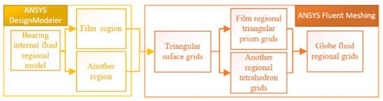
Figure 1.
Flow chart for the generation of the global fluid domain mesh model.
2. Prototype Design and Theoretical Performance Model
Empirical formulas for structure design of hydrostatic-guideway bearings are obtained from a large amount of actual engineering experience; therefore, the expected supporting load capacity, stiffness and damping can be achieved approximatively. In this study, the supporting load capacity must be no less than 1000 N. The conventional structure of the bearings shown in Figure 2 was designed based on the recommendation in the design manual for hydrostatic bearings [1].
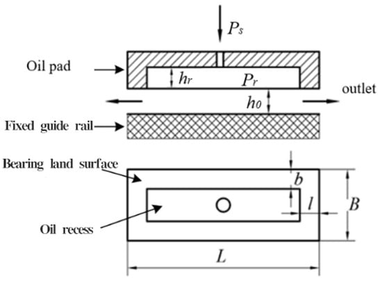
Figure 2.
Schematic diagram of structural parameters.
The lubricant Mobil-Velocite-10 was selected to reduce system temperature. To reduce recess deformation, a lower recommended value of recess pressure was adopted. The bearing width was selected according to the maximum supporting load capacity. The seal band width was selected at the minimum power consumption. In order to increase the bearing stiffness, a smaller recess depth was selected within the optional range. The detailed parameters are shown in Table 1 and a three-dimensional structure for the experiment is shown in Figure 3. At the top of the model, there is a spherical hinge constraint, which ensures that the structure can be rotated at will around the center of the ball. In the experiment, oil is injected from the oil inlet and flows through the right-hand orifice into the oil recess. Underneath the oil recess, an oil sealing surface is used to seal the oil.

Table 1.
Structural and oil parameters of hydrostatic bearings.
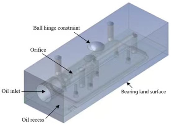
Figure 3.
CAD model of the hydrostatic bearing.
2.1. Supporting Capacity
The equivalent area corresponding to the pressure of rectangular recess can be expressed as [1]:
and the flow resistance of the bearing is determined by the oil viscosity and film thickness, written as:
where is oil dynamic viscosity; h is film thickness.
When orifice parameters, oil type, bearing structure size and oil supply pressure are determined, supporting load capacity, F is a function of film thickness:
is the pressure of the recess. K can be calculated as:
is density of oil, is orifice flow coefficient and is diameter of orifice.
2.2. Stiffness
Hydrostatic bearing stiffness is the capacity of oil film to resist displacement. It is expressed as the force required per unit displacement, which is also a function of film thickness, h, written as [1]:
where intermediate variable, can be calculated as:
is the dynamic viscosity of oil; is supply pressure.
2.3. Damping
Hydrostatic bearing damping can also be writen as a function of the film thickness, h [1]:
is the recess perimeter, is the recess area in the horizontal direction and is seal band area.
The above performance check results and analysis are shown in Section 5.
3. Simulation Model
3.1. Flow Governing Equations
The oil is governed by a modified N–S equation. In the Reynolds average method, the mean value and fluctuating components are used together to represent the solution variables of the instantaneous N–S equation, written as [1]:
where represents a scalar quantity, such as velocity or pressure.
In the inertial frame, substituting the variable expression in this form into the continuity and momentum equations with a time (or ensemble) average value, the global average momentum equation can be obtained. This can be represented as Cartesian tensors:
while u is the velocity of the element, Fi is the external volume force in direction of is a Kronecker symbol.
Equations (9) and (10) have a similar structural form to N–S equations, in which the solution variables are expressed as averages. The additional term represents the influence of turbulence, namely, the Reynolds stress. The Reynolds stress associated with the average velocity gradient is the common solution provided by the Boussinesq hypothesis [29]:
The Boussinesq hypothesis applied in the - model has the advantage of relatively low computational cost and is related to the calculation of turbulent viscosity, -t, which is calculated as a function of k and . The assumption of isotropic turbulent viscosity is generally applicable to shear flows governed by only one turbulent shear stress. This includes many technical flows, such as the wall boundary layer, mixed layer, jet flow, etc. It is exactly in line with the flow-field characteristics of hydrostatic bearings. Without high-intensity rotational flows and secondary flows, Reynolds stresses can be appropriately modeled by the Boussinesq hypothesis.
Since the standard - model was described by Launder and Spalding [30], it has become the main tool for practical engineering process calculation. The transport equations for and are obtained by exact equations and physical reasoning, respectively. The model’s robustness and accuracy make it popular in fluid dynamics and flow pattern analysis. Although many scholars have judged that the flow pattern inside the bearings is a laminar flow according to the Reynolds number, it was found that a large number of vortices and turbulence phenomena exist in the global fluid domain through pre-experimentation with the laminar flow model, and the residual convergence rate of the standard - model is better than that of the laminar flow model.
In the standard - model, the equations for and can be written as:
The term denotes the production of turbulence kinetic energy. According to the transport equation of , the term can be written as:
to calculate in a way that conforms to the Boussinesq hypothesis:
where is the average strain rate tensor modulus, which can be expressed as:
and the turbulence viscosity is calculated as:
The model constants C, C, C, and are widely used with the following values
These values have been determined from experiments for turbulent flow models, and have been found to work quite well in a wide range of wall-bounded and free shear flows.
3.2. Dynamic Mesh Governing Equation
In order to identify the relationship between supporting load capacity and film thickness, the transient motion control conservation equation was added to the oil film bottom surface and its parallel grid layers. Its integral form can be written as [1,31]:
is a scalar, V is an arbitrary control volume, is fluid density, is the velocity vector, is the velocity of the moving grid, is the diffusion coefficient, is the source term of the scalar and ∂V is the boundary of the control volume.
Equation (19) is a differential discretization of the integral form of the time derivative term, where we treat as a discretization performed by one variable. This discretization is independent of whether or not either the density or the velocity potential is a constant variable. The first-order forward difference formula can be used for a slow-moving oil film boundary to reduce the computational cost, and the time derivative term can be expressed as:
t is the time interval.
The derivative of volume with respect to time of control volume is computed from:
where is the number of faces on the control volume, is the volume swept out by the control volume face j over the time interval t and is velocity of the moving mesh.
The triangular prism grid is applied to subdivide oil film regions, which can be compressed and moved with the original high quality, thus ensuring the accuracy of the simulation. In the quasi-static analysis of the static supporting load capacity, the oil film bottom surface velocity will disturb the static supporting load capacity, but this can be avoided by defining a smaller velocity. The motion rule of the film’s bottom surface is described by the user-defined functions (UDFs).
3.3. Generation of Mesh Model for Global Fluid Domain
The model and local grid are described in Figure 4; all surfaces except for the inlet and outlet were defined as walls. The initial oil film thickness was 0.0301 mm, the recess depth was 1.5 mm, the pipe diameter was 4 mm, and the orifice diameter and length were 0.3 mm and 1 mm, respectively.
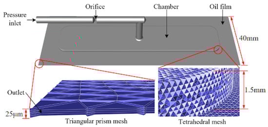
Figure 4.
Fluid domain model and grid detail view.
Due to the complexity of the global fluid domain model, it is difficult to use conventional methods to generate a high-quality structured grid. In order to make the simulation efficient and accurate, this study proposes the automatic dividing method for the unstructured grid. First, divide the global fluid domain by the unstructured surface grid with a maximum feature size of 0.2 mm and a minimum of 0.01 mm; it is necessary to ensure that the skewness values of the oil film upper and lower surfaces are similar. Then, the thin volume mesh is applied to stratify and subdivide the film region to obtain the triangular prism grid. Finally, automatically subdivide the other regions by the tetrahedral grid.
The high quality and low quantity of the mesh model were testified by the pressure distribution of the simulation shown as Figure 5. When the film region was stratified in five layers, the value of maximum-skewness and the number of cells in the oil film region were 0.518 and 1,391,350, respectively; in the other oil region, the values were 0.806 and 2,241,398 respectively.
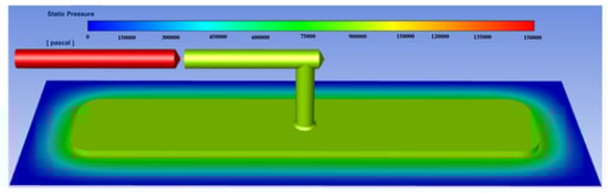
Figure 5.
Pressure profile of bearing interior (Film thickness h = 25 m).
The steady-state initialization was carried out by referring to the partial settings in Table 2; then, the dynamic mesh parameters were set. The supporting load capacity can be obtained by transient numerical analysis, as shown in Figure 5. The pressure distribution of 25 m film thickness in the simulation process was captured, as shown in Figure 5, which shows that the pressure distribution is uniform and reasonable, indicating that the mesh model meets the requirements of numerical analysis.
Table 2.
Detailed boundary conditions and input parameters.
3.4. Boundary Conditions
The N–S equations can be solved efficiently based on the finite element method (FEM). Czaban A [32] found that supporting load capacity considering non-Newtonian power-law properties is lower than that of ideal Newtonian fluid, about 10% lower. In order to simulate the internal flow field of hydrostatic bearings accurately, the rotary rheometer model MCR302 was used to measure the viscosity of Mobil-Velocite-10, which was fitted with power-law functions to obtain the exact viscosity characteristic of the oil. The relationship between the oil dynamic viscosity and shear rate can be expressed as [33]:
where is the viscosity consistency index and n is the viscosity power-law index.
For the tetrahedral grid, the fluid flow does not keep the same direction as the grid edge, so second-order discretization is generally used to obtain higher accuracy results. The detailed boundary conditions and input parameters of the simulation are shown in Table 2, and the structural and working parameters of hydrostatic bearings are derived from the recommended values.
4. Experimental Condition
In this paper, hydrostatic guideway bearings need to have high supporting capacity and stiffness to ensure that ultra-precision machine tools have very high machining precision. For this reason, the recommended oil film thickness between the bearings and the guideway is only 20 m, and a tiny change in film thickness can lead to large fluctuations in supporting capacity. It is difficult to accurately capture micro-size changes by conventional displacement sensors, which have uncertain signal identification errors and external vibration interference. In order to reduce the influence of system error on experimental results, a standard feeler gauge was adopted to measure film thickness.
In the experiments, oil was injected from the inlet and flowed into the oil recess through the orifice on the right side of the oil channel. In order to prevent oil from escaping through the gap on the lower side during the experiments, an oil sealing surface was used underneath the oil recess. At the same time, to ensure the stability of the structure, the structure was tightly fitted by means of open screws and bolts [28].
Figure 6 shows the experimental device and the testing conditions. Samples of different thicknesses with size differences less than 1 m were selected from a large number of standard feeler gauges before the experiment, constituting the pass gauge and stop gauge for each film thickness dimension. During the experiment, the film thickness was controlled by the displacement loading device and was identified by the feeler gauge samples.
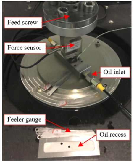
Figure 6.
Experimental devices and test conditions.
The range and resolution of the force-measuring instrument for measuring the supporting load capacity were 5000 N and 1 N, respectively. The bearings used in the experiment were connected with the loading rod by a ball hinge to maintain a uniform oil film thickness.
5. Verification and Application
5.1. Compared Results
The results of theoretical calculation, the simulation and the experiment are shown in Figure 7. The supporting load capacities of the three methods reflect the same trend; they increase with the decrease of film thickness. Evaluating the supporting load capacity of each thickness, the theoretical calculation results are much higher than the experiment results, and the average relative error between them is 22.70%. The error between the simulation and the experiment is 10.76%. However, when a larger load is applied, the loading force acts more like a concentrated load on the bottom of the ball hinge, so the edge part of the oil-sealing surface will be slightly deformed; in order to avoid the above effects, the experiments used the treatment shown in Figure 6. The average film thickness measured at a quarter position of the bearing length shown in Figure 6 has a certain influence on the results. Moreover, the smaller the film thickness, the larger the repeated measurement fluctuations for supporting load capacity will be, which is mainly due to the higher stiffness and the seal surface warping.
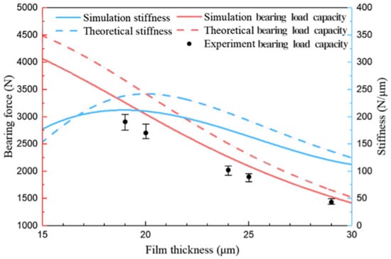
Figure 7.
The results of theoretical calculation, simulation and experimentation for supporting load capacity and stiffness.
Due to the limited experimental conditions, it was not possible to obtain the bearing force for each oil film thickness, so we obtained the bearing force for the five film thicknesses and made a dot plot. The bearing stiffness is actually the rate at which the supporting capacity varies with film thickness. As depicted in Figure 7, the curve-simulation bearing load capacity is close to the experimental bearing load capacity, Therefore, the effectiveness of the simulation of bearing capacity was verified. Further comparison between the simulated bearing capacity and the theoretical calculated bearing capacity curve shows that the simulated bearing capacity is closer to the actual value.
From the comparison of results, there is a large gap between theoretical results and the experiment in terms of supporting load capacity, so the theoretical calculation usually only plays a guiding role in the design. The supporting load capacity can be obtained accurately since the important factors of the numerical analysis, such as the geometric model, boundary conditions and the oil characteristics, are all consistent with the real situation.
5.2. Frequency Sweep Analysis for Bearing Damping
In order to identify the bearing damping based on perturbation theory, DMT was used to make the film bottom surface perform harmonic vibration at a linear swept frequency with a frequency range of 1–100 Hz and an amplitude of 1 m. The film bottom surface velocity was defined by DEFINE CG MOTION in the macroinstruction of UDFs, which can be expressed as:
In addition, to a certain extent, the higher the vibration frequency, the lower the fitted error. The reason is that the data points are more concentrated on both sides of the fitted line. When the film surface velocity is 0 m/s, the bearing stiffness is 208.3 N/m, and it is consistent with the results in Figure 7. This shows that the damping value obtained by numerical analysis is reliable due to the strict governing equation of the dynamic mesh.
Figure 8 shows that the simulation residuals were kept at about and the residuals of all variables were the same order of magnitude as the convergence of steady-state calculations, indicating that error terms introduced by the simulation have little fluctuation and can be ignored. After processing the time-variant data of supporting load capacity, the relationships between supporting load capacity, film bottom surface velocity and simulation time were obtained, as in Figure 9. Purple, red and green lines represent the relationship of time and wall, bearing force and wall velocity, and time and bearing force, while the blue line shows the relationship between time, bearing force and wall velocity, respectively. CFD results are recorded in Figure 10 when the oil pad is moved up and down by the UDF procedure, as described in Equation (23). The film surface velocity and corresponding supporting load capacity were approximatively fitted to a linear function, as in Figure 10. The slope of the straight line represents the damping. The average damping of the bearings with the film thickness of 20 m is 3.86 N·s/m obtained from the slope of the fitted line, in the same order of magnitude, with a theoretical calculation result of 6.62 N·s/m.
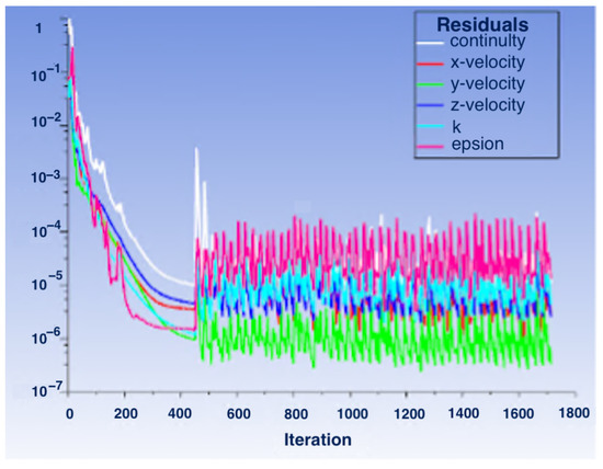
Figure 8.
The simulation residuals.
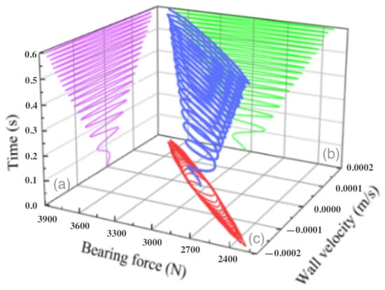
Figure 9.
Relationships between supporting load capacity, film surface velocity and simulation time: (a) relationship between film surface velocity and simulation time; (b) relationship between supporting load capacity and film surface velocity; (c) relationship between supporting load capacity and film surface velocity.
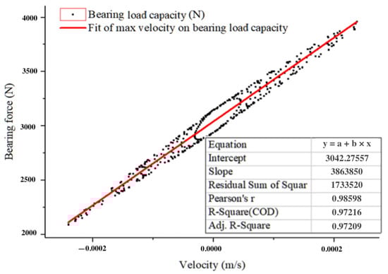
Figure 10.
Linear fitting of the supporting load capacity with maximum film surface velocity.
5.3. Vortex Analysis and Suppression
A large number of researchers, limited by the grid division, have used a simplified model of hydrostatic bearings for analysis of the flow field. However, our preliminary research found that the simplified model does not effectively reflect the real vortex situation. So we here compare the simplified model with the real model for analysis; a large number of vortices can be seen in the recess of the simplified model. The flow pattern inside the simplified model was obtained, as shown in Figure 11. The structure and simulation parameters are consistent with the above model, and only the orifice is simplified to aim at the oil recess. The pressure distribution is shown in Figure 12, which is consistent with Figure 5. It indicates that the supporting load capacity performance cannot change. However, a large number of vortices can be seen in the recess of the simplified model. This flow pattern is in agreement with the universal flow law after the jet flow directly impinges on a wall; it is similar to that described in the literature [10,12] and verified by the tracer particle experiment [12]. Therefore, the mesh model and input parameters used in this study can simulate flow pattern well and may be more accurate than a simplified flow-field model.
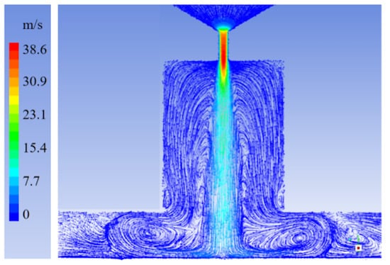
Figure 11.
Flow pattern of simplified model at recess inlet.
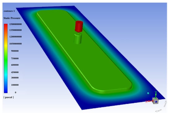
Figure 12.
Pressure profile of simplified model (film thickness h = 25 m).
Relevant studies have shown that vortices have an adverse effect on bearing stability [11,17]. Based on the viscous shear theory, a thin septum with double slits was designed and installed between the recess and the oil film to separate the fluid domain for blocking the influence of shear flow. Figure 13 shows the improved bearing structure. The thin septum with double slits is installed at the bottom of the original recess. To prevent the septum from reducing the supporting performance, an auxiliary recess with a depth of 0.1 mm is left under the septum. The basic principle is to combine the advantages of deep and shallow recesses, which are a uniform pressure distribution with higher value and suppression of the vortices, respectively.
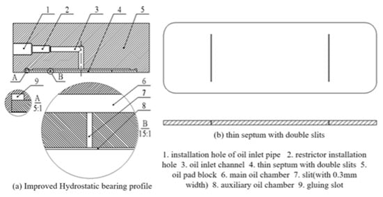
Figure 13.
Improved hydrostatic bearing structure.
The mesh generation method proposed in this paper is applied in the improved bearing analysis. Figure 14 shows the bearing internal fluid domain after improvement and its pressure distribution without significant change compared with Figure 5, so the supporting load capacity and stiffness of the bearings cannot change. The vortices in the improved recess are significantly reduced, and the obvious vortices only appear at the slit position of the thin septum, as shown Figure 15i1. All visible vortices are entirely suppressed, as shown in Figure 15i2 and Figure 15j2, with the adjustment of the slit width from 1 mm to 0.3 mm by image analysis of vortex position. Therefore, we conclude that the double slits can reduce vortices, and the reduction of slit width also suppress vortixes. Thus, this structure is expected to enhance bearing stability in higher speed conditions for ultra-precision machine tools.
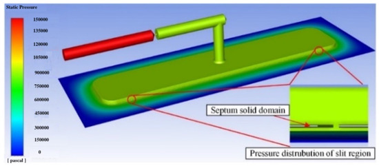
Figure 14.
Pressure distribution of the bearings at rest after optimization (film thickness h = 20 m).
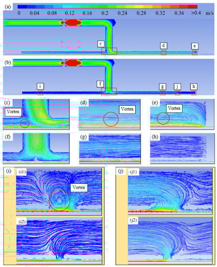
Figure 15.
Velocity flow pattern of the bearings at moving speed of 0.4 m/s. (a) Bearing recess without improvement. (b) Bearing recess with double-slit septum. (c,f) Recess inlet position. (d,g) Random local region. (e,h) Recess edge region. (i,j) Slit regions. (i1,j1) Slits with 1 mm width. (i2,j2) Slits with 0.3 mm width.
6. Conclusions
This article is about the use of a CFD method, as well as 3D meshing, in the analysis of load capacity, stiffness and damping of hydrostatic bearings. By comparing it to the traditional empirical formulae, it was found that the 3D meshing and CFD analysis is more accurate and can adapt to the analysis of various shapes of hydrostatic bearings, solving the analysis problem that the traditional empirical formulae cannot adapt to the new structure of hydrostatic bearings [28]. Through the steps of bearing design, analysis and optimization, the application value of this approach is presented.
- The self-adaptive generation of the global fluid domain mesh model can solve the problem of mesh generation for the model with multi-scale geometric dimensions, and can also increase the efficiency of mesh model processing. Moreover, the maximum skewness of the grids is less than 0.8, which can make the calculation results accurate. Due to the low number of grids, the performance of current personal computers is sufficient to handle the numerical analysis of the mesh model with high efficiency;
- With the help of the above mesh model processing method, the supporting capacity, stiffness and damping were captured by the simulation and verified by the experiment, and were more accurate than the results of theoretical calculation. Thus, this method can make the optimization of the hydrostatic bearing structure more diverse and the analysis more convenient;
- In this study, the flow pattern of the global fluid domain inside the bearings was depicted based on the proposed mesh generation method, and vortices were discovered in the recess. A double-slit septum was installed between the recess and the oil film to suppress the visible vortices without bearing performance attenuation. The structure improvement, combining the advantages of deep and shallow recesses, is expected to make hydrostatic bearings more stable in high-speed conditions for ultra-precision machine tools.
Author Contributions
Conceptualization, H.W. and Y.R.; investigation, H.W. and Y.R.; writing—original draft preparation, H.W. and Y.W.; writing—review and editing, Y.W., H.W. and Y.R.; supervision, H.W. and Y.W. All authors have read and agreed to the published version of the manuscript.
Funding
We acknowledge support from the Science Challenge Project (No. TZ2018006-0102-03), the National Natural Science Foundation of China (No. 51875223) and the National Key Technologies Research and Development Program (2020YFB2007600).
Data Availability Statement
Not applicable.
Acknowledgments
We thank Xuedong Chen for use of the laser displacement sensor.
Conflicts of Interest
The authors declare no conflict of interest.
References
- Rowe, W.B. Applications of the metacentre and of the general pressure equations, pressure of gases. In Hydrostatic, Aerostatic and Hybrid Bearing Design; Elsevier: Oxford, UK, 2012. [Google Scholar]
- Liu, Z.S.; Zhang, G.H.; Xu, H.J. Performance analysis of rotating externally pressurized air bearings. Proc. Inst. Mech. Eng. Part J J. Eng. Tribol. 2009, 223, 653–663. [Google Scholar] [CrossRef]
- Khatri, C.B.; Sharma, S.C. Influence of textured surface on the performance of non-recessed hybrid journal bearing operating with non-Newtonian lubricant. Tribol. Int. 2016, 95, 221–235. [Google Scholar] [CrossRef]
- Zhang, G.J.; Li, J.; Tian, Z.X.; Huang, Y.; Chen, R.C. Film Shape Optimization for Two-Dimensional Rough Slider Bearings. Tribol. Trans. 2015, 59, 17–27. [Google Scholar] [CrossRef]
- Shen, F.; Chen, C.L.; Liu, Z.M. Effect of Pocket Geometry on the Performance of a Circular Thrust Pad Hydrostatic Bearing in Machine Tools. Tribol. Trans. 2014, 57, 700–714. [Google Scholar] [CrossRef]
- Liang, P.; Lu, C.H.; Pan, W.; Li, S.Y. A new method for calculating the static performance of hydrostatic journal bearing. Tribol. Int. 2014, 77, 72–77. [Google Scholar] [CrossRef]
- Shao, J.P.; Zhou, L.M.; Li, H.M.; Yang, X.D.; Zhang, Y.Q.; Chi, M.S. Influence of the oil Cavity Depth on Dynamic Pressure Effect of Hydrostatic Thrust Bearing. In Proceedings of the 2009 International Conference on Intelligent Human-Machine Systems and Cybernetics, Hangzhou, China, 26–27 August 2009; pp. 11–14. [Google Scholar]
- Shao, J.P.; Liu, G.D.; Yu, X.D. Simulation and experiment on pressure field characteristics of hydrostatic hydrodynamic hybrid thrust bearings. Ind. Lubr. Tribol. 2018, 71, 102–108. [Google Scholar] [CrossRef]
- Xu, X.Q.; Shao, J.P.; Yang, X.D.; Zang, Y.Q.; Yu, X.D.; Gao, B.W. Simulation on Multi-oil-cavity and Multi-oil-pad Hydrostatic Bearings. Appl. Mech. Mater. 2013, 274, 274–277. [Google Scholar] [CrossRef]
- Gao, S.Y.; Cheng, K.; Chen, S.J.; Ding, H.; Fu, H.Y. CFD based investigation on influence of orifice chamber shapes for the design of aerostatic thrust bearings at ultra-high-speed spindles. Tribol. Int. 2015, 92, 211–221. [Google Scholar] [CrossRef]
- Zhang, Y.Q.; Fan, L.G.; Li, R.; Dai, C.X.; Yu, X.D. Simulation and experimental analysis of supporting characteristics of multiple oil pad hydrostatic bearing disk. J. Hydrodyn. 2013, 25, 236–241. [Google Scholar] [CrossRef]
- Horvat, F.E.; Braun, M.J. Comparative Experimental and Numerical Analysis of Flow and Pressure Fields Inside Deep and Shallow Pockets for a Hydrostatic Bearing. Tribol. Trans. 2011, 54, 548–567. [Google Scholar] [CrossRef]
- Tauviqirrahman, M.; Jamari, J.; Susilowati, S.; Pujiastuti, C.; Setiyana, B.; Pasaribu, A.H.; Ammarullah, M.I. Performance Comparison of Newtonian and Non-Newtonian Fluid on a Heterogeneous Slip/No-Slip Journal Bearing System Based on CFD-FSI Method. Fluids 2022, 7, 225. [Google Scholar] [CrossRef]
- Rasep, Z.; Yazid, M.N.; Samion, S. A study of cavitation effect in a journal bearing using CFD: A case study of engine oil, palm oil and water. J. Tribol. 2021, 28, 48–62. [Google Scholar]
- Tauviqirrahman, M.; Jamari, J.; Wicaksono, A.A.; Muchammad, M.; Susilowati, S.; Ngatilah, Y.; Pujiastuti, C. CFD Analysis of Journal Bearing with a Heterogeneous Rough/Smooth Surface. Lubricants 2021, 9, 88. [Google Scholar] [CrossRef]
- Shang, Y.; Cheng, K.; Ding, H.; Chen, S.; Samion, S. Design and Optimization of the Surface Texture at the Hydrostatic Bearing and the Spindle for High Precision Machining. Machines 2022, 10, 806. [Google Scholar] [CrossRef]
- Ghezali, F.; Bouzidane, A.; Thomas, M. 3D Numerical investigation of pressure field of an orifice compensated hydrostatic bearing. Mech. Ind. 2017, 18, 101. [Google Scholar] [CrossRef]
- Li, D.Y. Study on CFD solution method for static characteristics of hybrid oil film bearing. Appl. Mech. Mater. 2012, 155–156, 236–240. [Google Scholar] [CrossRef]
- Hou, Z.Q.; Xiong, W.L.; Yang, X.B.; Yuan, J.L. Study on Dynamic Characteristics of a Hydrostatic and Hydrodynamic Journal Bearings for Small Diameter Grinding Spindle. Adv. Mater. Res. 2012, 497, 99–104. [Google Scholar] [CrossRef]
- Li, Q.; Zhang, S.; Ma, L.; Xu, W.W.; Zheng, S.Y. Stiffness and damping coefficients for journal bearing using the 3D transient flow calculation. J. Mech. Sci. Technol. 2017, 31, 2083–2091. [Google Scholar] [CrossRef]
- Liu, C.P.; Hu, J.P. A magnetorheological hydrostatic guideway system for machining vibration control. J. Braz. Soc. Mech. Sci. 2019, 41, 12. [Google Scholar] [CrossRef]
- Lin, Q.Y.; Wei, Z.Y.; Wang, N.; Chen, W. Analysis on the lubrication performances of journal bearing system using computational fluid dynamics and fluid-structure interaction considering thermal influence and cavitation. Tribol. Int. 2013, 10, 8–15. [Google Scholar] [CrossRef]
- Cui, C.; Guo, T.N.; Wang, Y.J.; Dai, Q. Research on Carrying Capacity of Hydrostatic Slideway on Heavy-duty Gantry CNC. AIP Conf. Proc. 2017, 1839, 020159. [Google Scholar]
- Wang, W.; Cheng, X.H.; Zhang, M.; Gong, W.W.; Cui, H.L. Effect of the deformation of porous materials on the performance of aerostatic bearings by fluid-solid interaction method. Tribol. Int. 2020, 150, 106391. [Google Scholar] [CrossRef]
- Wen, Z.P.; Wu, J.W.; Tan, J.B. An adaptive modeling method for multi-throttle aerostatic thrust bearing. Tribol. Int. 2020, 149, 105830. [Google Scholar] [CrossRef]
- Maamari, N.; Krebs, A.; Weikert, S.; Wild, H.; Wegener, K. Stability and dynamics of an orifice based aerostatic bearing with a compliant back plate. Tribol. Int. 2019, 138, 279–296. [Google Scholar] [CrossRef]
- Helene, M.; Arghir, M.; Frene, J. Numerical study of the pressure pattern in a two-dimensional hybrid journal bearing recess, laminar, and turbulent flow results. J. Tribol. 2003, 125, 283–290. [Google Scholar] [CrossRef]
- Wu, H.; Huang, Y.; Cui, H.; Rong, Y. A passive compensated method with hydraulic transmission for static infinite stiffness of thrust bearing. Tribol. Int. 2021, 163, 107193. [Google Scholar] [CrossRef]
- Hinze, J.O. Reference book for research of mechanics of turbulence. In Turbulence; McGraw-Hill Publishing Co.: New York, NY, USA, 1975. [Google Scholar]
- Launder, B.E.; Spalding, D.B. Research of predictions of turbulent flow. In Lectures in Mathematical Models of Turbulence; Academic Press: London, UK, 1972. [Google Scholar]
- Berry, R.A.; Saurel, R.; LeMetayer, O. The discrete equation method (DEM) for fully compressible, two-phase flows in ducts of spatially varying cross-section. Nucl. Eng. Des. 2010, 240, 3797–3818. [Google Scholar] [CrossRef]
- Czaban, A. CFD analysis of hydrodynamic pressure distribution in non-Newtonian oil in journal bearing lubrication gap. Solid State Phenom. 2015, 220–221, 37–42. [Google Scholar] [CrossRef]
- Bharti, R.P.; Chhabra, R.P.; Eswaran, V. Steady flow of power law fluids across a circular cylinder. Can. J. Chem. Eng. 2006, 84, 406–421. [Google Scholar] [CrossRef]
Publisher’s Note: MDPI stays neutral with regard to jurisdictional claims in published maps and institutional affiliations. |
© 2022 by the authors. Licensee MDPI, Basel, Switzerland. This article is an open access article distributed under the terms and conditions of the Creative Commons Attribution (CC BY) license (https://creativecommons.org/licenses/by/4.0/).