A Deep-Learning-Based Multi-Modal Sensor Fusion Approach for Detection of Equipment Faults

Abstract

Condition monitoring is a part of the predictive maintenance approach applied to detect and prevent unexpected equipment failures by monitoring machine conditions. Early detection of equipment failures in industrial systems can greatly reduce scrap and financial losses. Developed sensor data acquisition technologies allow for digitally generating and storing many types of sensor data. Data-driven computational models allow the extraction of information about the machine’s state from acquired sensor data. The outstanding generalization capabilities of deep learning models have enabled them to play a significant role as a data-driven computational fault model in equipment condition monitoring. A challenge of fault detection applications is that single-sensor data can be insufficient in performance to detect equipment anomalies. Furthermore, data in different domains can reveal more prominent features depending on the fault type, but may not always be obvious. To address this issue, this paper proposes a multi-modal sensor fusion-based deep learning model to detect equipment faults by fusing information not only from different sensors but also from different signal domains. The effectiveness of the model’s fault detection capability is shown by utilizing the most commonly encountered equipment types in the industry, such as electric motors. Two different sensor types’ raw time domain and frequency domain data are utilized. The raw data from the vibration and current sensors are transformed into time-frequency images using short-time Fourier transform (STFT). Then, time-frequency images and raw time series data were supplied to the designed deep learning model to detect failures. The results showed that the fusion of multi-modal sensor data using the proposed model can be advantageous in equipment fault detection.

1. Introduction

Industry 4.0 has encouraged a paradigm shift from automation to autonomy by introducing the significance of artificial intelligence (AI) technologies. The workforce in factories that have adopted Industry 4.0 concepts has gradually decreased, and production efficiency has increased. The more labor-intensive tasks in factories, such as maintenance, has also been affected, and the companies have recognized the value of AI-assisted maintenance programs. Conventionally, maintenance programs are implemented in two parts: planned or unplanned maintenance. An unplanned breakdown of machines during manufacturing causes disruptions in the production process and causes scrap. As a result, the production capacity is affected, and financial losses can be experienced depending on the cycle time plan and the number of affected lots per unit of time. It is almost impossible to compensate for these losses if a piece of critical equipment in a manufacturing step is affected. Especially-high-volume manufacturing companies have placed safeguards in their production where critical equipment is constantly monitored with intelligent fault detection and classification (FDC) systems. An FDC system constantly monitors equipment conditions with various sensors and generates early warnings. Early prediction of incipient equipment faults can give engineers enough time to take action and satisfy the longest possible equipment uptime.

In an FDC system, a critical component is the generation of fault models and alarm rules so that false positive alarms are minimal. A new trend is to incorporate data-driven fault detection models by utilizing machine learning (ML) and efficiently processing multiple machine sensor data to increase robustness and accuracy in fault detection and classification. Generally referred to as condition monitoring (CM), this method is now replacing unplanned maintenance approaches and has been adapted with significant contributions of ML and deep learning (DL) models. Instead of relying on manually created alarm rules, an intelligent CM with a deep learning model can send an alert when it detects a change in machine health, allowing the maintenance technicians to intervene on time. The challenge remains in designing accurate, intelligent models that can leverage all sensors and achieve maximal equipment fault coverage. Since different equipment fault modalities can be prominent in different sensors and it can be difficult to know them in advance, data obtained from a single sensor may be insufficient for an effective CM approach. Furthermore, depending on the fault type, sensor data in a different signal domain can reveal more discriminative features; however, these may not be known in advance. Therefore, multi-sensor and information fusion concepts can play an important role in this field to achieve maximal fault detection coverage for equipment.

Sensor fusion refers to the methods used to combine information from several sensors. This approach can allow compensation of weaknesses over one sensor and help to improve the overall accuracy or reliability of a fault classification. Relying on single sensor data can be detrimental in cases such as in the presence of noisy data affected by process conditions, in the event of a sensor failure or selection of a sensor type that does not capture fingerprints of a particular equipment fault condition. In these highly likely situations, sensor fusion techniques allow for obtaining more robust results from multiple sources of information.

The data sources for the fusion process may not always be identical. Depending on the types of sensors utilized in fusion, the approach can be divided into two topics: heterogeneous and homogeneous sensor fusion. In heterogeneous sensor fusion, the data to be fused is obtained from different sensors, e.g., vibration and current, while for homogeneous sensor fusion, the data is obtained from the same sensors, e.g., vibration X, Y, and Z axes. Depending on the step where the sources of information are fused, it can be categorized as data-level fusion, feature-level fusion, and decision-level fusion [1].

Multi-modal learning for sensor fusion can involve associating information from multiple sensors and their different sensor data domains. For example, while a vibration sensor can reveal the most critical information on mechanical equipment anomalies, a current sensor may also contribute to detecting similar failures. A transformation of sensor data into different domains, e.g., frequency domain, can contribute to the detection of certain faults and provide additional modalities as well. Considering that one piece of equipment has many different fault types, the ability to incorporate multi-sensors and multi-domain information for equipment condition monitoring can be valuable in the field.

Recent research work in the literature has shown the strength of data-driven DL models in sensor fusion; however, effective multi-sensor fusion strategies with multi-modal data are rare. This study proposes a DL model that supports heterogeneous feature-level sensor fusion and a multi-modal learning structure. The main motivation is to design a model that can cover different equipment faults in a single model. Instead of designing individual models for each fault type, one model can have better usability in practice for condition monitoring applications. The model’s effectiveness in detecting equipment faults was experimentally verified with artificially induced common equipment faults in electrical motors. Multi-sensors consisting of vibrational and current data collected from two independent testbed setups were utilized with both their time and time-frequency domain representations.

The rest of the paper is organized as follows: firstly, a literature review of related work in condition monitoring and sensor fusion applications is presented. Secondly, a background on the theory of the methods used is introduced to the reader. Afterward, the proposed method and details of the model design process are presented together with an introduction of the experimental testbed setup where the datasets are collected. Then, the results obtained from the experimental studies are presented with a discussion. Finally, the conclusions and future studies that will follow this study are presented.

2. Related Work

AI for condition monitoring has been a very active field in the literature. Furthermore, equipment fault detection has been a popular use-case for developing new ML or DL models by researchers due to the significant benefits for manufacturing. Liu et al. [2] reviewed the use of AI models in fault detection of rotating machinery. The models, such as kNN, naive Bayes, SVM, and deep learning were investigated based on model advantages and disadvantages. In a recent work, Peng et al. [3] surveyed the existing methods of fault detection and recognition of fault types on rolling bearings from vibration data.

Although ML techniques have produced successful results, the powerful feature extraction capabilities of deep learning techniques have made them more popular. Hoang et al. [4] conducted a study on deep-learning-based error detection in bearings and presented powerful methods using autoencoders, a restricted Boltzmann machine, and CNNs. Furthermore, Zhang et al. [5] performed a very comprehensive study on deep-learning-based fault detection on bearings. They investigated the techniques found in the literature such as CNNs, deep belief networks, RNN, and GANs, and the most widely used open-source datasets.

Recent developments in sensor technologies have enabled frequent usage of condition-based monitoring to capture frequently occurring faults in equipment. Although dynamic physics-based mathematical models can be developed for monitoring equipment parts for fault detection [6] in production, this approach might require expert knowledge and might have limited equipment coverage. On the other side, data-driven DL-based modeling strategies have gained significant attention and recent studies have demonstrated successful results for FDC modeling. Among these studies, many of them have utilized the power advantage of convolutional neural network (CNN)-based model design. The ability to learn powerful features from raw data through convolutional operations is the main strength of CNN-based algorithms in FDC applications [7,8]. However, a known major drawback of a CNN model is the requirement for a large amount of training data [9]. For example, Zhang et al. [10] presented a systematic review of the current literature based on transfer learning as a remedy for CNNs’ need for a large amount of data. In addition, different strategies are being developed by researchers in the field to alleviate this drawback through effective sensor fusion strategies. Karabacak et al. [11] applied the GoogLeNet model to classify incipient equipment faults after collecting thermal images from healthy and defective worm gears. Vibration and sound signals were collected from the sensors, and the data were converted into spectrograms. When the results were examined, it was observed that thermal images gave better results than vibration and sound sensor data. Santo et al. [12] proposed a hard disk health status definition that combines an automated approach with ML prediction techniques based on the LSTMs. It can be observed that the method tested on two different data sets has achieved successful results. Al-Dulaimia et al. [13] proposed a hybrid model running LSTM and 1D-CNN in parallel to estimate the remaining useful life of turbofan engines. The proposed method aimed to provide past time information with a LSTM structure and to extract spatial features with a 1D-CNN structure. Yao et al. [14] proposed a deep convolutional neural network based on a multi-scale structure with an attention mechanism. When the results were examined, it was observed that the multi-scale learning structure outperformed the single-scale models. Additionally, it was observed that the attention mechanism added to the multi-scale structure increased the model accuracy. Although the study was successfully conducted and the analysis of the vibration signal was significant, the study was only limited to a single type of sensor.

Among the most frequently encountered sensor data used for equipment fault detection in the literature are vibration and current. These types of signals may contain useful information in both time and frequency representations. Wang et al. [15] trained DCNN models with four different signal representations to test the effect of different signal representations’ success in classifying gearbox failures. Depending on the data structure, these representations, such as time domain, frequency domain, time–frequency domain, and the reconstructed phase space, were trained with 2D or 1D CNNs. When the results were examined, the most successful method was the frequency domain with 1D CNNs. Lee et al. [16] trained state-of-the-art image classification models such as GoogLeNet, AlexNet, and ResNet50 to classify different motor failures after converting triaxial acceleration data into 2D images (spectrograms) using the power spectral density function. Although these studies test the effectiveness of different signal representations in fault detection, their limitation is that they rely on a single type of sensor for equipment fault detection.

A single data sensor for industrial fault detection may not always be clean and high-quality. This is a major problem, especially when relying on a single sensor for equipment fault detection in production. Alternatively, data from multiple sensors can also be fused to improve classification accuracy. Compared to single-sensor data, multi-sensor signals can often provide better information that can be used for fault detection [17]. Nasir et al. [18] investigated power, sound, vibration, and acoustic emission (AE) signals and studied the optimal combination of sensors by conducting different experiments with sensors utilizing classical ML methods. XGBoost algorithm gave the highest accuracy for two different combinations. First, a combination of power and acoustic emission sensors, and then a combination of power, acoustic emission, and microphone sensors were studied. These two combinations gave the same accuracy with 0.923. After adding the microphone, the false-positive rate decreased from 0.091 to 0, but the false-negative rate increased from 0.067 to 0.133. This work showed an effective method for CM, although it was limited in terms of accuracy by using ML instead of DL. Gültekin et al. [19] proposed a new deep-residual-network (DRN)-based fusion approach to diagnosing failures under varying bearing conditions. The proposed model uses time-frequency representations converted by short-time Fourier transform from time series data obtained from different sensors as input. When the obtained results are examined, it is seen that the presented approach is more effective than a single-type sensor. Li et al. [20] designed a deep adaptive channel layer for fault detection in helicopter transmission systems and studied which data from different sensors are more important and which are less important. The authors proposed weighing sensors according to their importance. It has been observed that 100% accuracy is achieved when the proposed method is trained with focal loss, which is suitable for unbalanced data sets. However, one sensor that is known to be critical for a specific fault can be not so effective in a different fault type. Gong et al. [21] proposed a novel method for detecting faults in bearings, consisting of data level fusion and CNN-SVM. First, they segmented the vibration time series data and made it two-dimensional. Then, they combined the two vibrational signals, which were reconstructed in 2D, and made them two channels to perform data level fusion. Kou et al. [22] investigated the classification of tool wear status using vibration, current and infrared images for a tool condition monitoring system. In this work, raw time domain vibration and current data were converted to images using the GADF [23] method. The images of the different signals obtained were classified with the CNN model created by data level fusion. When the results were examined, the fusion method was more successful than the other nonfusion method, achieving an accuracy result of 91%. However, the model did not consider different signal representations of sensor data. Patil et al. [24] performed manual feature extraction from vibration and acoustic emission signals to detect various forms of misalignment under different operating conditions. The extracted features were ranked according to their importance with ANOVA, and feature selection was made. When the selected features were tested with machine learning algorithms, it was observed that 100% accuracy was achieved with SVM however, the main drawback is that manual feature extraction, and ranking may not be practical for production monitoring.

Linear prediction coefficients (LPC) and mel-frequency cepstral coefficients (MFCC) are signal processing techniques commonly used in fields such as sound processing and fault recognition. Habbouche et al. [25] proposed two methodologies based on these signal processing techniques. In addition, to examine the importance of the fusion method, early-level fusion was performed with the LPC-LSTM method. The results showed that the MFCC-CNN-LSTM method achieved higher success, but the fusion-applied LPC-LSTM method was more successful than single sensor methods and achieved 100% accuracy, showing the strength of multi-sensor fusion. Das et al. [26] present two different feature extraction methods that were applied to infrared thermal images (IRT) to classify the surface contamination level of metal oxide surge arresters (MOSAs). Firstly, the features were extracted with the ResNet50 deep neural network. Secondly, to obtain superpixel features the Slic [27] algorithm was used. Then, feature selection was carried out according to the ANOVA test from these features and fused. Classical machine learning algorithms classified the fused features. The random forest algorithm gave the most successful results when the obtained results were examined. In addition, feature fusion gave more successful results than using them individually, supporting the power advantages of sensor fusion in the field.

Within the examined literature work, a study that can provide a single global model to support different equipment faults and can incorporate heterogeneous sensors, especially with different domain representations has not been encountered.

3. Theory and Background

The proposed model utilizes fundamental CNN layers. A classical CNN model architecture consists of convolutional, activation, pooling, and batch normalization layers for feature extraction stages and fully connected layers for classification stages. In this section, these fundamental components of CNN architecture are introduced together with signal transformation techniques, which are applied to collected equipment sensor data.

3.1. Convolutional Neural Network

3.1.1. Convolutional Layer

The Convolutional Layer is the main building block of a CNN. It provides the extraction of local features by applying certain convolution filters that slide over the input signal. Different weights in the applied filter will allow different features to be extracted from the signal, and many different filters are utilized for feature extraction in a CNN. The Convolutional Layer can extract both low-level and high-level features from a signal. The convolution process can be explained as follows:

$$y\left[m,n\right]={\displaystyle \sum }_j {\displaystyle \sum }_{i}x\left[m,n\right]\ast h\left[m-i, n-j\right]$$

(1)

where y denotes the output signal of size m × n and x is the input signal. A convolutional kernel operator of size i × j is denoted by h.

3.1.2. Activation Layer

In a CNN, after a convolution process, the resulting data, which is also called a feature map, is usually passed through an activation layer. This type of layer applies a non-linear transformation to the signal. It provides advantages such as improving the representation ability of the network, ease of computation, and speed in convergence. Although there are various activation functions, the Rectified Linear Unit (ReLu) function is the most widely used one.

3.1.3. Pooling Layer

The pooling layer is frequently added in CNN architecture. It reduces the network’s parameters and the amount of computation by reducing the size of the input signal. Although there are various pooling methods, the most commonly used is the max pooling method.

3.1.4. Batch Normalization

This technique was first introduced in a study published by Ioffe and Szegedy [28]. Batch normalization (BN) is a normalization operation between layers of a neural network. BN is usually applied after the Convolutional Layer and before the activation function. The network can be made to learn at fewer epoch values by applying batch normalization. On the contrary, a known disadvantage is that it can shorten the network’s training process. Furthermore, it can also significantly stabilize the training process and achieve higher accuracy in fewer epochs.

3.2. Short Time Fourier Transform (STFT)

STFT is used as a signal transformation technique and displays a change in frequency components of a signal over time. It is one of the most widely used transformation techniques in equipment fault detection. STFT is based on discrete Fourier transformation (DFT) that enables the transformation of a signal from the time domain into the time-frequency domain for a time-dependent signal. It can capture the varying frequency and phase components over time. To calculate the STFT, the signal is divided into segments with windows of equal length, and then the Fourier transform for each short segment is calculated separately. Equation (2) shows a mathematical expression of STFT: X is the STFT transformation of the input signal $x_n$ at time n within the m-size windowed block and $w_n$ is the window function. The frequencies over which DFT is calculated is represented by ω.

$$\mathrm{STFT}=X\left(m,w\right)={\displaystyle \sum }_{-\infty }^{\infty }{x}_n{w}_{n-m}{e}^{-j\omega n}$$

(2)

A visual representation of STFT can be obtained using spectrogram images. A spectrogram shows the frequency spectrum amplitude changes of a signal in varying colors over time.

3.3. Sensor Fusion

The sensor fusion process, one of the sub-topics of the Information Fusion term, is applied to eliminate uncertainties in data and make more stable and accurate predictions. Data from a single source may not always be sufficient for decision-making in cases such as failures in a data source or noise in the data due to several operational situations. It is also possible that different types of sensors can reveal different information about the environment. Sensor fusion is used in many engineering applications such as autonomous driving and condition monitoring to enhance decision-making with more information gain. Depending on the fusion level, sensor fusion can be classified into three main categories. These are defined as data-level fusion, feature-level fusion, and decision-level fusion.

3.3.1. Data Level Fusion

This is a sensor fusion technique that combines data obtained at the raw data level. It works at the lowest level as compared to other categories. Data Level Fusion is generally used to fuse data with the same physical properties obtained from homogeneous sensors. Differentiated data from heterogeneous sensors are combined at higher levels [29].

3.3.2. Feature Level Fusion

The data obtained from each data source enters the fusion process after independent discriminative features are extracted from the raw data. The fusion is realized by combining the extracted feature vectors.

3.3.3. Decision Level Fusion

In this fusion technique, which is the highest fusion level, a final decision is made by combining the decisions that have already been derived individually by using various features from individual sensors.

4. The Proposed Method

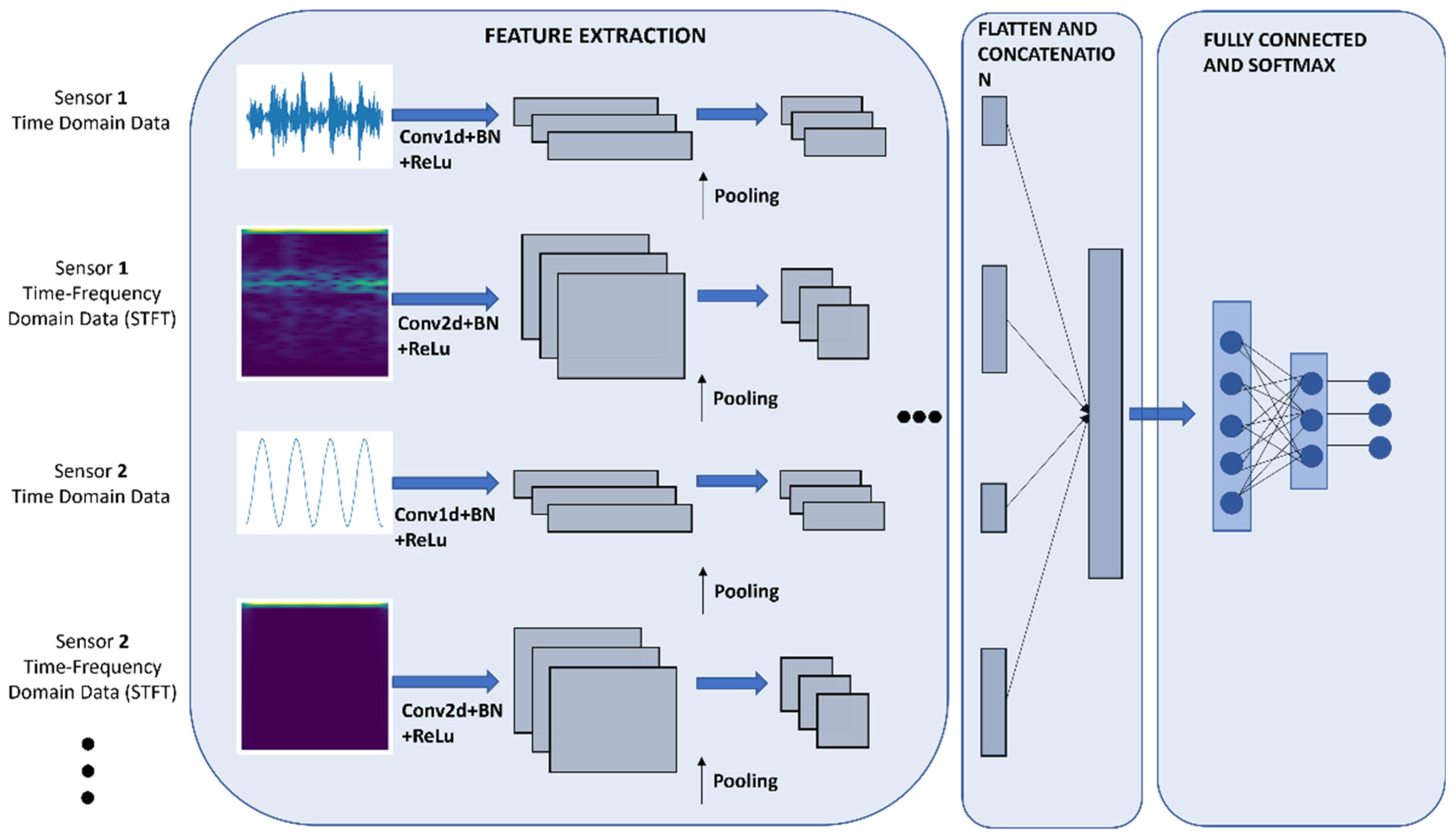
An illustrative figure for the proposed method is shown in Figure 1. The proposed method includes more than one CNN-structure working together and can incorporate multiple heterogenous sensors and information from their different domain representations. In the following subsection, the multi-modal approach, the multi-sensor fusion approach and the proposed multi-modal sensor fusion structure obtained by combining these elements will be introduced.

Figure 1. The proposed DL model structure.

Multi-Modal Sensor Fusion Approach

Multi-modal learning involves associating more than one subject while trying to make sense of something. For example, a student can learn a subject from both images and text. However, by combining the two, better learning can be achieved with the link between images and texts. Multi-modal learning provides dynamic learning through the interaction of different resources.

In this study, a multi-modal approach was leveraged for a global model by using different types of sensor data and their different domain representations. The main motivation behind this approach is that, in equipment condition monitoring, each sensor type can include critical information depending on the fault type being investigated, which is not known in advance. Additionally, some sensor data may reveal more prominent fault fingerprints in a different domain, e.g., frequency, than in the time domain, depending on the nature of the signal.

For example, vibration is a mechanical phenomenon in which oscillations occur around a point of equilibrium. These oscillations, recorded over a certain time are called vibration signals. If a piece of equipment has an incipient defect, harmonics around the fundamental frequency start to appear in collected vibration signals [30]. Therefore, processing the raw time domain of a vibrational signal might not reveal critical information as much as its frequency domain representation. An STFT transformation of a signal can provide both amplitude and frequency components and time transition of these harmonics.

Similarly, although a current sensor can reveal important information on electrical faults in a motor, some of the high-frequency effects can also be observed in the current signal when a mechanical fault occurs. Alternatively, time domain statistical features of a current signal can also reveal some critical information. A deep learning model that can fuse all this information and simultaneously incorporate multi-modal sensors can be invaluable in overcoming these challenges. The proposed method has been developed for this reason. The model offers a multi-modal learning structure and shows that different information sources can be combined effectively in an equipment condition monitoring application.

The proposed model uses vibrational and current sensors collected from two independent electrical motor experimental testbeds; however, the model can also be expanded to different equipment types and their faults. For raw time domain data, 1D CNNs were used, and for the STFT transformed spectrogram time-frequency images, 2D CNNs were used.

As shown in Figure 1., after taking both time series data and frequency representations of each sensor data as input and extracting the feature vectors with 1D and 2D CNNs, these vectors were combined with a concatenation layer, and feature-level fusion was carried out. Then, a single feature vector belonging to four different data types combined was passed through fully connected layers and classified. After each convolution step, batch normalization and ReLU were applied as activation functions. In the last layer, the Softmax function was applied as the activation function for the classification step.

Three convolutional blocks were added after each input. Each convolution block consists of convolution, BN, ReLU, and max pooling layers. A 3 × 3 kernel was applied for 2D CNNs. The filters’ sizes were determined as 32, 64, and 128, respectively. To suppress possible noise in the first layers and apply large kernel sizes to obtain better features, 64 × 1 kernel and 4 × 1 stride were applied in the first layer. After the first layer, a 3 × 1 kernel was applied. The filters were determined as 8, 16, and 32, respectively. Max pooling kernel sizes were determined as 2 × 2 for 2D and 2 × 1 for 1D. After the vibration spectrogram, vibration time domain, current spectrogram, and current time domain inputs were processed and flattened in parallel, and feature vectors of 4608 × 1, 384 × 1, 4608 × 1, and 384 × 1 dimensions were obtained, respectively. By concatenating these feature vectors, a new vector with the size of 9984 × 1 was created. Then, for the classification stage, it was passed through fully connected layers of 512, 256, 128, and n (class number) sizes, respectively. ReLU was used in the first three layers in the fully connected layers, and Softmax activation function was used in the last layer.

5. Experiments

In this work, the data needed to verify the proposed model was obtained by artificially induced faults utilizing two independent testbeds. The testbeds were designed to realize electrical motors’ rotating parts, such as bearings. However, other motor faults can also be mimicked utilizing these testbeds. One of the testbed datasets is known as the Paderborn University (PU) dataset and is publicly available. The second dataset was obtained from an in-house custom-made testbed in our research center laboratory at the Eskisehir Osmangazi University (ESOGU). In the following section, the data collection setups for both PU and ESOGU are introduced.

5.1. The ESOGU In-House Dataset and Experimental Data Collection Setup

An in-house experimental testbed, as shown in Figure 2, was used to create artificially induced fault scenarios. For varying motor conditions, three types of sensor data can be collected. These are vibration, current and torque signals. A National Instrument (NI) data acquisition system CompactRIO 9539 was used for data collection and recording. For vibrational signals, a three-axis vibration sensor (PCB triaxial 356A15) was mounted on the front of the motor. Only the z vibrational axis was utilized in this study. Three-phase AC-motor current signal was also recorded during motor operation. The magnetic powder break was used to create a motor load and mimic varying loading conditions of motor operation.

Figure 2. ESOGU in-house testbed setup used to create motor fault scenarios.

The fault scenarios examined in this study included motor bearing parts. These are rotating parts of a motor and they are most prone to break-down. As shown in Figure 3, various types of faults were induced into bearing parts in different locations by creating holes at varying depths. If a fault is created on the outer race of the bearing, it is called an “outer” fault. Depending on the depth of the whole, the fault class is given a name. For example, the “outer-0.5” fault type indicates a damaged bearing on the outer race of the bearing with a 0.5 mm hole depth. The holes were created by using a high-precision arc cutting tool, and varying depths in a range of 0.5–1.5 mm were created to mimic severity of a fault type.

Figure 3. Example of artificially created fault classes on bearings for the in-house dataset.

5.2. The Paderborn (PU) Dataset and Experimental Data Collection Setup

This publicly available dataset was generated from a testbed as shown in Figure 4 [31]. The experimental setup consists of test drive electric motors (left-side) as well as a synchronous servo motor as a load motor (right-side). The torque and rotational speed measurements were obtained through the torque sensor located on the shaft. Artificial bearing errors were created with a rolling bearing test module located in the middle of the testbed. The vibration of the bearing was measured using a piezoelectric vibration sensor (Model No. 336C04, PCB Piezotronics, Inc., Depew, NY, USA) with a 64 kHz sampling rate. Motor phase current was measured with a current transducer (LEM CKSR 15-NP) at a 64 kHz sampling rate.

Figure 4. Paderborn university dataset experimental testbed setup.

The entire dataset consists of 32 experimental sets, including motor current and vibration data. In this dataset, 6 sets were obtained from healthy bearings, 12 sets were from artificially damaged bearings, and 14 were from real damaged bearings. In addition, each experimental set was repeated under varying four electrical motor test conditions. These conditions are:

(1)

Speed of 1500 rpm and torque 0.7 Nm, bearing radial force of 1000 N;

(2)

Speed of 900 rpm and torque of 0.7 Nm, bearing radial force 1000 N;

(3)

Speed of 1500 rpm and torque of 0.1 Nm, bearing radial force 1000 N;

(4)

Speed of 1500 rpm and torque of 0.7 Nm, bearing radial force 400 N.

Note that only the operating condition (1) dataset was used in this study.

5.3. Data Preprocessing and Model Hyperparameters Setup

In the data preparation phase of the experimental ESOGU dataset, 120 s of recordings were taken so that 6200 samples were obtained from 6400 current signals from the vibration signal per second. A total of 8 files were obtained under full load conditions for different hole depths of 0.5 and 1.5 mm for the healthy, outer ring, inner ring, and ball classes. Each file contained 768,000 data samples for vibration and 750,000 for current. For calculating STFTs, each measured signal was divided into non-overlapping windows. The window size was determined as 512 for vibration data and 500 for current data to obtain an equal amount of data from both signals. The 65 × 65 spectrograms were obtained from the signals of the divided window. To facilitate the calculation, the last row and column of the 65 × 65 spectrogram were truncated to 64 × 64 dimensions. A total of 10,000 of the 12,000 total data samples were used for the training; the remaining 2000 data samples were divided into 1000 for tests and 1000 for validations.

In preparing the PU dataset, a total of 256,000 data samples were divided into 512 non-overlapping windows, similar to our own dataset, and obtained 500 data samples for each file. A total of 16,000 data samples were obtained from 32 different files representing each of our classes. The 64 × 64 spectrograms were obtained by repeating the steps applied in the dataset to obtain the spectrograms. In total, 70% of the total data was divided into the training phase. The remainder of the data were divided into tests and validations with a 50% ratio. When both the ESOGU and PU datasets were divided into train, validation, and test sets, these sets were kept unchanged across different fusion method trials. For example, only the current time domain data for the ESOGU dataset was kept constant, in addition to the two-input current time and time-frequency domain cases. Similarly, only vibration time-frequency domain data was the same across all methods whenever vibrational STFT was needed for the input method.

The initial learning rate for the training of both datasets was determined as 1 × 10⁻⁴. Adam was used as the optimization algorithm. The step-based learning rate scheduling function regulated the learning rate parameter. For the step-based learning rate scheduling function, the drop rate was set to 0.5 and the step size to 10.

For model building and training, the Google Colab platform was used. The code was written with Python 3.7.13. Tensorflow 2.8.2 was used to build the proposed deep learning model. In addition, the system included a Tesla T4 15.1 GB GPU and 13.61 GB RAM.

6. Results and Discussions

Firstly, the proposed model was tested on the PU dataset and afterward on the in-house (ESOGU) dataset to diagnose the condition of the bearings in electrical motors. Different combinations of inputs were used to test the effectiveness of fusion on our proposed method. For example, “multi-sensor time and time-frequency domain” refers to the four inputs entered into the proposed method with one channel vibrational axis raw data in the time domain and its STFT transformed spectrogram image, as well as current sensor raw time and STFT transformed image. A visual representation of STFT spectrogram image data for ESOGU dataset is shown in Figure 5.

Figure 5. Example of STFT spectrograms for each class in the ESOGU dataset.

Individual accuracy results were obtained where each experiment was repeated five times for both data sets in every method. For the in-house dataset, 100% success was achieved in all trials when the four-input method was used. For the PU data set, an average of 97.10% was obtained. The mean ± std of other methods are listed in Table 1.

Table 1. Comparison of DL models for various types of sensor data and different datasets. Accuracy (%) values are the mean ± std over five trials.

Methods	PU Dataset			ESOGU Dataset
	Accuracy	Std	F1 Score	Accuracy	Std	F1 Score
Multi-sensor time and time-frequency domain (4 inputs)	97	±1.45	0.96	100	0	1
Vibration time and time-frequency domain (2 inputs)	84	±0.5	0.87	100	0	1
Current time and time-frequency domain (2 inputs)	89	±2.57	0.89	97	±0.83	0.97
Only vibration time domain	79	±1.18	0.79	87	±2.28	0.80
Only vibration time-frequency domain	80	±0.99	0.80	99	±0.44	0.99
Only current time domain	61	±7.68	0.61	77	±7.63	0.74
Only current time-frequency	57	±0.99	0.58	66	±4.94	0.60

Figure 6 and Figure 7 present the loss plots over each dataset. The plots were captured while training the dataset with all four inputs. When the graphs were examined, it was observed that the training and validation progressed in good harmony for both data sets. The proposed method’s generalization capacity was sufficient and reached high accuracies in a short time, as shown in the testing results.

Figure 6. Loss-epoch graph of the proposed method on the ESOGU in-house dataset.

Figure 7. Loss-epoch graph of the proposed method on the Paderborn dataset.

To better analyze the classification results, the confusion matrices of the proposed algorithm are presented in Figure 8 and Figure 9. In the confusion matrices, each row and column represents the predicted and true classes. Diagonal and off-diagonal cells indicate the number of correctly and incorrectly classified observations, respectively. The confusion matrix obtained with the ESOGU dataset can be seen in Figure 8. Healthy and bearing failure type (inner and outer) and the depth of hole (0.5 mm or 1.5 mm) are given. For example, a bearing fault class created on the outer race of the bearing with a 0.5 mm hole is indicated with a label “outer 0.5”. When Figure 8 is examined, it can be observed that all of the classes were predicted correctly without any misclassification. The confusion matrix obtained with the PU dataset is given in Figure 9. Each fault class code number (0–31) and its corresponding fault type is listed in Table 2. For example, the fault class code 0 corresponds to a healthy bearing class, whereas the fault class code 21 corresponds to an artificially damaged bearing fault at the inner race location. The PU dataset was utilized to test the classification performance of the model as the number of equipment fault classes scaled up. Although there are false classifications for a few samples in the PU dataset, most of the predictions were made accurately for all classes at a high rate.

Figure 8. ESOGU dataset for seven-class confusion matrix.

Figure 9. Paderborn dataset with 32-class confusion matrix.

Table 2. The PU dataset fault class codes (0–31) and their corresponding fault class type.

		Artificially Damaged		Real Damaged
	Healthy	Inner	Outer	Inner	Outer	Inner + Outer
Fault Class Codes	0, 1, 2, 3, 4, 5	21, 22, 24, 25, 26	6, 7, 9, 10, 11, 12, 13	23, 27, 28, 29, 30, 31	8, 14, 15, 16, 17	18, 19, 20

Different input combination methods have been used to examine the effect of multi-sensor and multi-modal fusion structures. These methods are listed and enumerated by definition as follows:

(1)

An input method that takes raw data and spectrograms of only vibration data as input (two-input vibration);

(2)

Method that takes the raw data and spectrograms of the only current data as input (two-input current);

(3)

Method that takes only vibration spectrogram as input (only vibration spectrogram);

(4)

Method that takes only vibration raw data input (only vibration raw);

(5)

Method that takes only the current spectrogram as input (only current spectrogram);

(6)

Method that receives only current raw data input (only current raw);

(7)

Method that takes spectrogram and raw data of vibration and current sensors (four-input fusion).

Figure 10 and Figure 11 show the accuracy values vs. the trials made for all the input methods listed. When the results are examined, it can be seen that the vibration data for the in-house data set have better success compared to the current data, indicating that vibrational sensors are more discriminative in this equipment set. When only vibration spectrogram data were used, an average of 99% accuracy results were obtained. With the multi-modal learning approach to vibration data (1) and the proposed method, the obtained classification performance value reached 100%. The advantage of the proposed method can be seen better in the PU dataset. When a multi-modal learning structure is included in these methods, accuracy is higher across all trials than those with a single input. It has been observed that when the multi-modal learning structure and the multi-sensor structure are combined, they outperform other methods.

Figure 10. ESOGU dataset comparison with different methods.

Figure 11. Paderborn dataset comparison with different methods.

7. Conclusions

This work proposes a CNN-based deep learning model that can enable a multi-sensor fusion structure. The proposed method can combine multiple heterogeneous sensors and their data from different domains. As a power advantage, this enables users to obtain a global model that can be used in production for various types of equipment faults instead of training a single model for every fault type. Since the proposed model is agnostic to input sensor parameters and does not perform any weighting between sensor or data types in advance, the sensors that are not critical for the fault class may cause unnecessary computational expense for the user.

Experimental tests are performed utilizing vibration and current data and a multi-modal learning structure to diagnose the most commonly encountered electrical motor failures, called bearing failures. Five trials were conducted with a publicly available dataset, called the Paderborn University dataset in the literature, to observe how consistent the proposed method was. Additional in-house generated datasets were also utilized to confirm the proposed method’s effectiveness. The results showed that depending on the nature of the dataset, the proposed model can help to obtain better classification performance by combining multi-modal data from multi-sensors. In the results obtained from the ESOGU dataset, since vibration data was the most discriminative sensor data, the accuracies were able to reach up to 100% with the proposed method when multi-modal structure was established. Although using only vibration data was sufficient to achieve high accuracy, the results show that the model can still work stably when current data is also included. For the PU dataset, the advantage of the proposed method can be better seen. The proposed method produced the highest results with an accuracy of 97% and the model was 13% more successful than the closest method (two-input vibration) as well. The proposed method in the PU dataset outperformed the other benchmarking methods. These results show how effective the combination of multi-modal learning and multi-sensor could be with the proposed method.

As a future study, additional motor or other types of equipment faults will be experimented with, and the proposed method will be tested in different fault types with additional sensors. Furthermore, implementation of the proposed work for an edge-AI application will also be considered.