Abstract
The rendering of tensor glyphs is a progressive process of visualizing the vector space both in fluid dynamics and the latest medical scanning. Nowadays, the rendering accuracy is ensured by numerical methods based on interpolation of tensor functions. The tensor glyph functions to visualize significant properties of the vector space. Not all these properties are visualized at all times. The number of properties and their unambiguity depend on the method chosen. This work presents a direct analytical expression covering rank two tensors in a plane. Unlike the methods used so far, this method is accurate and unambiguous one for tensor visualization. The method was applied to the simplest tensor type, which presented an advantage for the method’s analytical approach. The analytical approach to the planar case is significant also because it provides instruction on how to expand analytical calculations to cover higher spatial dimensions. In this way, numerical methods for tensor rendering can be replaced with an accurate analytical method.
1. Introduction
The rendering of tensor glyphs is a progressive process of visualization in vector spaces. Tensor glyphs are objects that represent multidimensional data using several admissible rules [1]. The main uses are in visualizing tensors of fluid dynamics, stress tensors, or a Jacobian matrix of a velocity field [2], as well as diffuse tensors of magnetic resonance in medicine [3,4].
A rank two tensor glyph in 2D or 3D space must satisfy several requirements. The following requirements are fully satisfied in some glyph structures and satisfied only to a limited degree in others. The conditions to be satisfied by general tensors are invariance under isometric domain transformation, scaling invariance, direct encoding of real eigenvalues and eigenvectors, glyph uniqueness with respect to the relevant tensor, and continual glyph changes mapping continuous changes in the tensor.
Kratz et al. team focused on combining statistical and analytical methods, using especially Mohr diagrams in the area of stress tensors [5]. Some rendering techniques stemmed from knowledge of the tensor eigenvectors. With hyperstreamlining, these data were enhanced, thus improving the complexity of the visualization technology. However, the analysis was based on visualizing two-dimensional, scalar-derived charts, thus reducing information on tensor properties [6,7,8]. To proceed with the analysis of the entire tensor invariant part, Zobel and Scheuermann introduced the term extreme points [9].
Kindlmann and Schultz introduced superquadratic tensor glyphs that satisfy all of the requirements, but only where symmetric tensors are concerned [10,11].
In the work of Globus et al. [12], the condition of uniqueness was not satisfied, because only the real eigenvalues were represented in the form of an ellipsoid, and it did not hold for complex values. Similarly, Theisel et al. [13] showed glyphs that failed to satisfy the condition of uniqueness, as well as that of change continuity. Technical mechanics approaches the visualization of tautness tensors in several ways. Mohr circles [14] visualize only eigenvalues, and therefore lack constancy under rotation, which fails to satisfy the condition of invariance under isometric domain transformation. Lately, the research into tensor visualization has been exploring different metrics such as Frobenius, Euclidean, Wasserstein, and Fisher Rao [15].
All of the papers mentioned above address individual tensor properties through numerical methods, in which the results are made more exact through interpolation, subject to the preservation of the usual tensor invariants [16,17]. However, this condition is not satisfied at all times. Technical mechanics operate with, for example, the ellipse of inertia, [18], which violates the first tensor invariant, as pointed out below.
The ingenuity of the proposed method compared to the methods used so far lies in the accurate analytical calculation of tensor rendering. The proposed analytical calculation applied to rank two tensors in the plane is capable of precise rendering of all tensor properties in the form of an analytical tensor glyph.
We are not aware of the existence of a direct analytical calculation of a tensor shape in the form of graphic visualization. The analytical calculation proposed for rank two tensors in a plane makes it possible to accurately represent all tensor properties in the form of an analytical tensor glyph.
Analytical calculation of tensor glyphs was applied to the planar case, as it is the simplest one to compute. Section 2 describes decomposition of the general matrix into its symmetrical and antisymmetrical component. This facilitates further simplification of the analytical calculation with the sole focus on the symmetrical tensor. Section 3 presents how tensor invariants are determined, pointing out, among other things, the manner in which complex results in quadratic form can be represented by real numbers. Analytical calculations require the third invariant be defined, in addition to the two known tensor invariants, as it is directly related to the symmetrical matrix norm. The complete analytical procedure for tensor glyph computing is presented in Section 4. This section also features tensor glyph illustrations. Section 6 introduces a special tensor glyph shape, enabling measurement of the golden section proportions. The significance of this lies in the fact that such proportions will materialize under exactly the 45-degree angle of the reference vector viewed from the aspect of basic tensor glyph symmetry. This finding leads to new useful considerations, for example in terms of the optimization of topological structures in the field of materials strength [19].
2. Theoretical Background
All mathematical objects have underwent development that started with simpler objects. Before a tensor could be created, the vector needed to be defined. The vector definition was preceded by a scalar definition.
A multidimensional array can also be precisely described by an object of a tensor type. Tensor rank is determined from the number of simultaneous directions representing a physical value. It then follows that the number of tensor components is derived from the following formula:
where is the number of components, is the number of dimensions, and is the tensor rank.
For example, the definition of tensor rank for a 3D space is as follows. A tensor of rank is an array of values (in 3D space) called tensor components, which combine with multiple directional implicators (basis vectors) to form a quantity that does not vary with changes in the coordinate system [20].
Based on the above, a table of precisely defined tensor types and numbers of tensor components can be constructed (Table 1).

Table 1.
Number of spatial object components.
Higher dimensions are described in metric spaces by the defined spatial Pythagorean theorem. Spatial structures where the space dimension is smaller than the tensor rank are marked in grey. The position of planar tensors analyzed in the present paper is marked in green.
Most often, a tensor is defined as a multidimensional array. Formally, it is defined through indices that, subject to the observation of certain rules, enable transformation operations of matrix calculation [21]. The definition of a tensor as a multidimensional array satisfying the transformation law dates back to the work of Ricci [22]. Another tensor definition takes the form of a multilinear map. This definition better shows the independence of the tensor from its base in the geometric object sense [23,24]. In some mathematical applications, the tensor is defined based on the tensor product of vectors in a vector space. This definition leads to a tensor being an object without components, thus enabling the extension of the linear algebra concept to multilinear algebra [25,26].
According to Table 1, a rank two tensor in a plane has four components, which can be expressed in the form of a square matrix. This view leads to a simplified tensor definition, drawing on the planar case. The tensor definition derives from tensor components and the transformation prescription. The tensor components alone do not create a spatial object. A spatial object can emerge only if the tensor transformation is applied in every direction.
Building on this consideration, a tensor can be derived from the procedure used for rotating the vector or the coordinate system. The vector rotation involves a transformation element in the form of a special square matrix, with a functional relation existing between the individual values. This rotational matrix is not a tensor, but the calculation principle can be applied to tensors as well. A general tensor in a plane can be defined by four different real numbers, without a functional relation between the individual values. However, a mathematical decomposition of general matrices into their symmetric and antisymmetric parts is available.
Each general matrix, and hence the matrix of a general tensor, can be decomposed through a simple modification of the addition of the symmetric and antisymmetric tensors:
where is the symmetric tensor and is the antisymmetric tensor.
In terms of its size, the antisymmetric part does not depend on the general tensor’s symmetric part. The general matrix expression of the general tensor is as follows:
where represents the general tensor components, represents the symmetric tensor components, and represents the antisymmetric tensor components.
3. Invariants of the Tensor in a Plane and Tensor Eigenvalues
Rotating the coordinate system with respect to the initial state yields a square matrix, but the information about the initial state prior to rotation is lost. In the initial state, the initial vector is defined by angle . If the rotation angle is zero, then the components of the initial vector lie along the main coordinate axis. Unknown components of the initial vector, , are the eigenvalues of the transformation matrix that emerges from rotating the coordinate system, and this matrix is diagonal.
Despite varying angle , a rotational matrix always preserves the determinant (6). In this case, the matrix eigenvalues equal one, so the initial angle must equal 45°. However, as demonstrated below, a rotational matrix cannot be a tensor:
Let us generalize this requirement also for the tensor matrix, whose initial state can be expressed as the product of the eigenvalues and the identity matrix:
where is a square matrix and is an identity matrix.
Let the determinant of any tensor matrix remain constant, too. Then the difference between the matrices results in the characteristic equation, and the respective determinant equals zero.
The parameter in this equation is an unknown variable. Adjustments lead to a quadratic equation:
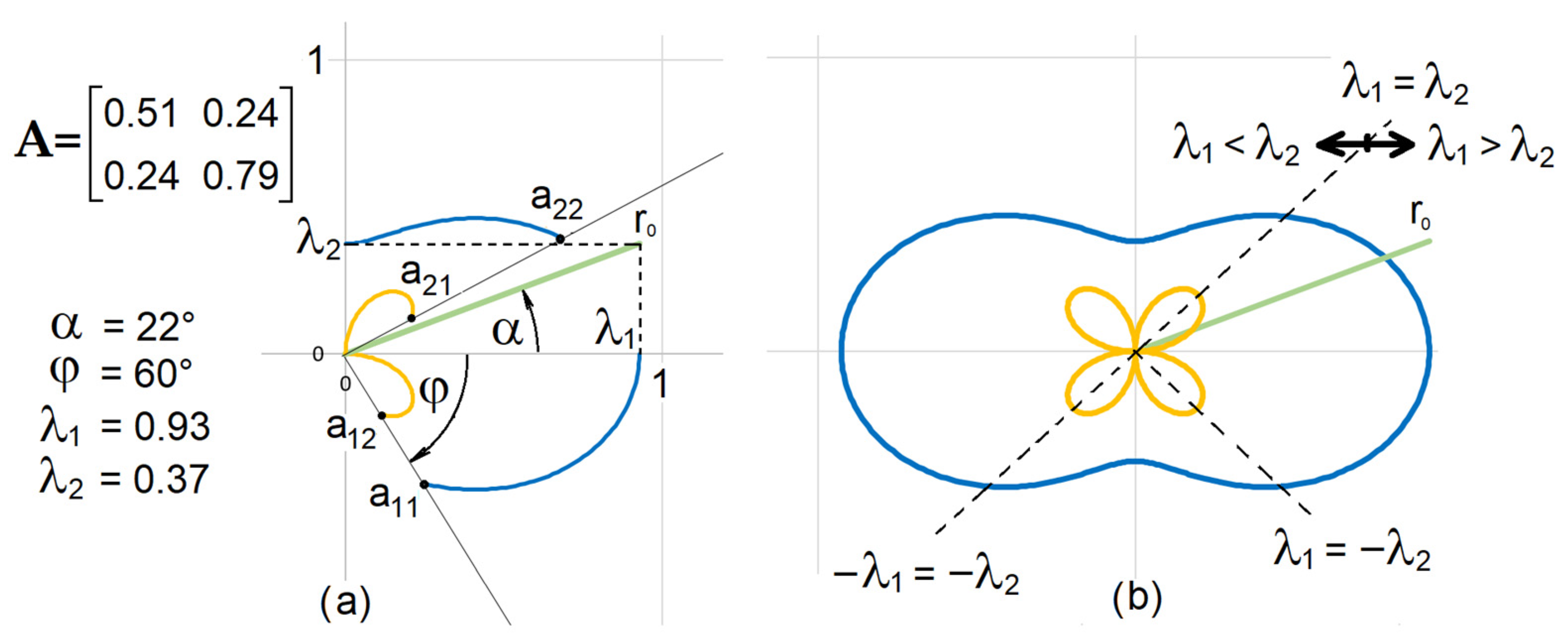
Solving the quadratic equation, we arrive at the unknown values of . To represent the shape, it is necessary to determine the domain of values for real roots only. The validity lies in the value interval of the initial angle , as shown in Figure 1.
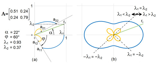
Figure 1.
Symmetric tensor and its components rotated by (a) and (b) .
The asymmetry of the domain of angle is due to its approximation to the domain of the quadratic equation. When the angle is larger than any enabled by the domain, the quadratic equation has complex roots.
Each tensor can be expressed as a polynomial, which is called the quadratic form. For a planar tensor, it is enough to solve a polynomial of the second order, which corresponds to the quadratic equation. The equation roots can be real or complex. Complex roots emerge when the eigenvalues satisfy . This exchange is the result of the parameters swapping their positions in the main diagonal square matrix. In such a case, the discriminant is a negative number and the corresponding matrix is negative-definite, because the eigenvalues do not change. Each complex solution matches exactly one real solution, which is arrived at by swapping the order of eigenvalues to satisfy . The eigenvalues’ order does not result in a loss of information from the swap of their position. Thus, visualization can have the same form in both real and complex solutions. By reshuffling the order of eigenvalues, a solution in the range of real numbers is arrived at, because the tensor matrix is positive-definite. Such a result can be represented graphically.
If we rotate the coordinate system with respect to the tensor’s initial state, the tensor’s transformation matrix components must duly change. The quadratic equation coefficients cannot change, because the initial state does not change either. These quadratic equation coefficients are called tensor invariants. Therefore, the following relations automatically hold for invariants:
Trace is the first invariant (sum of values of the main diagonal):
The determinant is the second invariant.
The above relations are commonly known. However, yet another tensor invariant exists, which has the form of the initial vector’s square length. This corresponds to the sum of the squares of the eigenvalues (15). The size of this vector stays unchanged during transformation.
The invariant in the form of the initial vector’s length can be expressed in absolute value:
or by its square, which does not change either:
Inserting it in the quadratic equations (Appendix A) and making adjustments, we arrive at the following result:
Further analysis uncovers the fact that the initial vector length corresponds to the symmetric part of the general matrix norm (Frobenius or Hilbert–Schmidt norm). A square symmetric matrix norm is as follows:
Inserting the components into the equation below (17) yields the same result:
In the literature, a matrix norm is not considered to be an additional tensor invariant. Nevertheless, the additional invariant is necessary for the analytical calculation of the tensor’s graphical representation.
The above formulas show that the rotational matrix maintains the determinant and the matrix norm, yet cannot be a tensor, as it does not satisfy the first invariant. This case is special because it must satisfy two conditions. Based on Equation (15) and the double root discriminant, we have:
It follows from these conditions that the following must hold for a rotational matrix:
Inserting and adjusting the components, we get:
which is satisfied only in the case of the rotational matrix; however, the first invariant requires a condition (11), which is not satisfied.
4. Analytical Procedure for Solving the Reverse Task
This section highlights the key to the tensor’s graphical representation. The previous task can be reversed in the sense that the rotation angle can be the unknown value and the parameters can be known.
This task is not addressed in practice in the way outlined here, likely due to the fact that to solve it, two invariants in the plane are not enough, and it is suitable to derive the solution for a symmetric tensor only. A general asymmetric tensor can be addressed only when the symmetric tensor has been solved.
Since this task is not commonly addressed in the literature, we outline the manner of deriving transformational relations. For unambiguous solving of the reverse task, the above-mentioned relations are used simultaneously with the condition of tensor symmetry:
The rotational angle of the coordinate system is determined with the help of the angle formed by the matrix eigenvector and the initial coordinate system. The eigenvector can be derived from relation (7). After having been multiplied by the eigenvector, the following holds true:
Only one eigenvector satisfies the above equality notation. Its orientation is determined by angle with respect to the initial tensor state. Making use of commonly known adjustments, we arrive at the following relation:
A symmetric tensor in a plane is unequivocally determined by three independent values. Rotating the coordinate system from its initial state will change the tensor components, but the tensor will remain the same; it will just be represented in a different direction. Thus, a tensor is an omnidirectional object. Based on this notion, the tensor shape can be represented in a plane through components under a given angle of the coordinate system’s rotation. Gradually changing the angle of rotation all the way to 360°, some shape characteristics of a symmetrical tensor should emerge in the plane.
Based on the above-mentioned formulas, the component can be expressed, resulting in a quadratic form after derivation (Appendix B):
One root of the quadratic equation corresponds to the initial state and the other to the state rotated by angle . In terms of solving the task, only the rotated state is of interest. Subsequently, the remaining components of the symmetric tensor are expressed as follows:
The graphical representation creates an omnidirectional shape of the symmetric tensor for the initial vector , as shown in Figure 1. Figure 1b shows the point of the mutual swap of the values on the main diagonal, so that the solutions of the equation be real numbers.
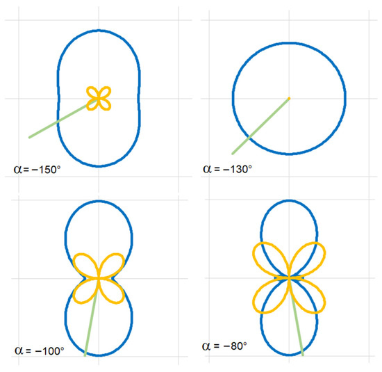
Figure 2.
Symmetric tensor glyphs: .
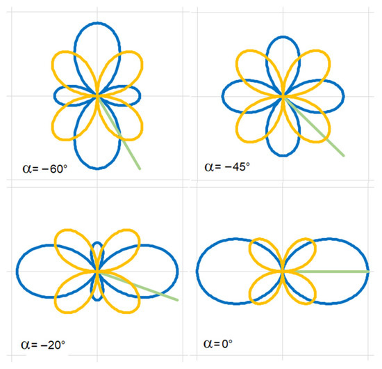
Figure 3.
Symmetric tensor glyphs: .
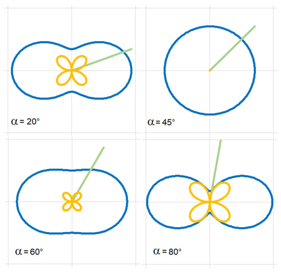
Figure 4.
Symmetric tensor glyphs: .
As shown, symmetric tensor glyphs repeat their shapes with changes in the initial angle. Different shapes are limited to a single quadrant.
5. General Tensor
The previous section introduced the symmetric tensor with three freely exchangeable components. The antisymmetric tensor features only one freely exchangeable component. Therefore, the only possible geometric shape corresponding to the antisymmetric tensor is a circle. If it should be a different shape, the tensor determinant would not be constant when rotated by angle , which would violate the tensor invariant condition.
When a general tensor is expressed in a matrix form, the antisymmetric tensor components do not change with changes in rotation angle . The absolute value of these constant components represents the circle’s radius:
The general tensor maintains the product of symmetric and antisymmetric tensor invariants:
with index representing the general tensor invariants, and and being the invariant indices of the symmetric and antisymmetric tensors, respectively. Applying the above formulas, the general tensor can be represented graphically, as shown in Figure 5 and Figure 6.
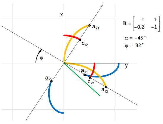
Figure 5.
General tensor components rotated by .
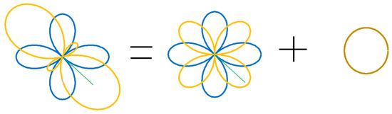
Figure 6.
General tensor is a product of symmetric and antisymmetric tensors, using parameters in Figure 7.
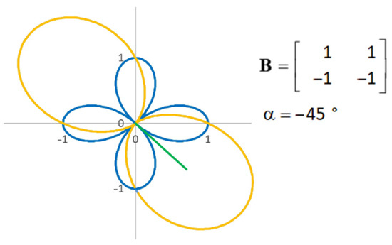
Figure 7.
General tensor with .
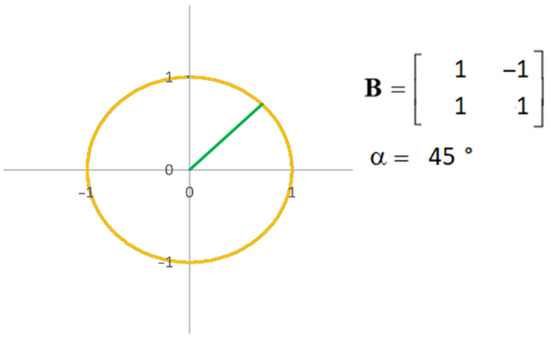
Figure 8.
General tensor with .
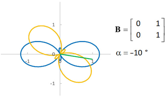
Figure 9.
General tensor with .
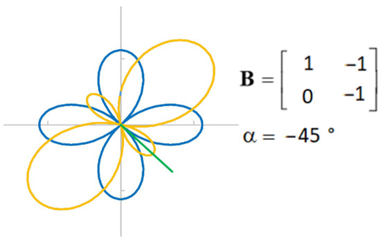
Figure 10.
General tensor with .
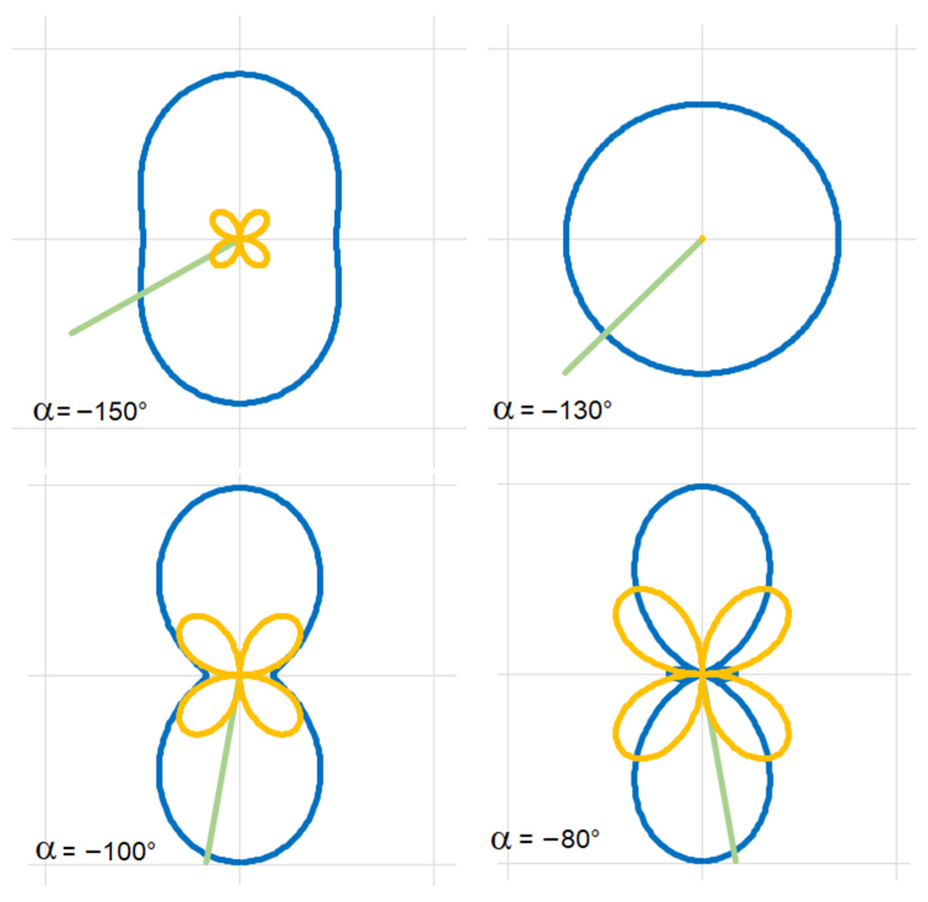
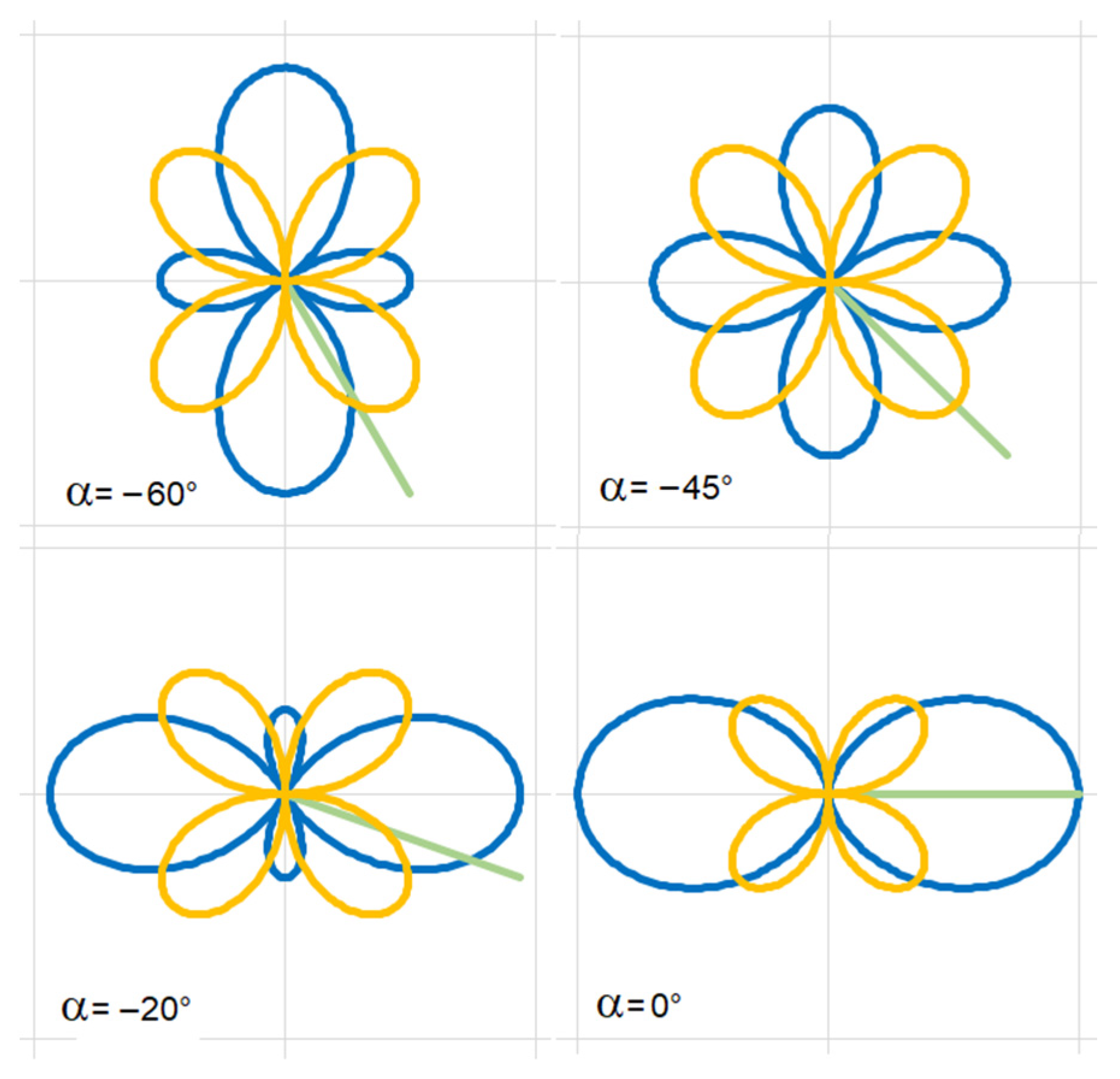
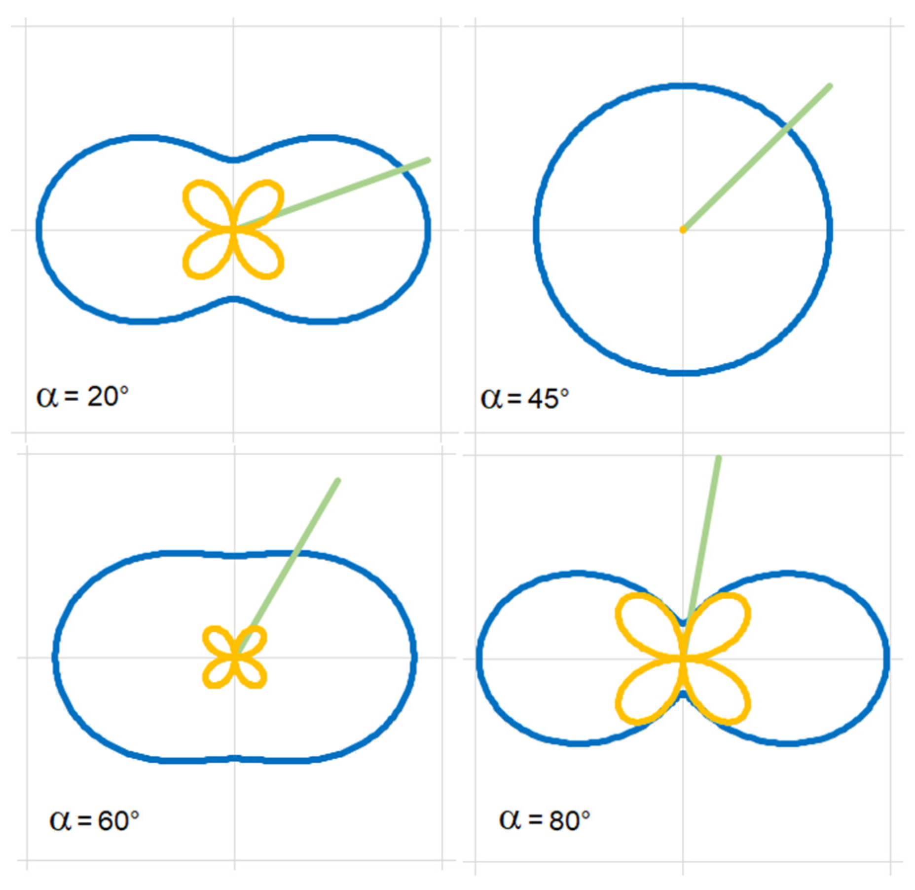
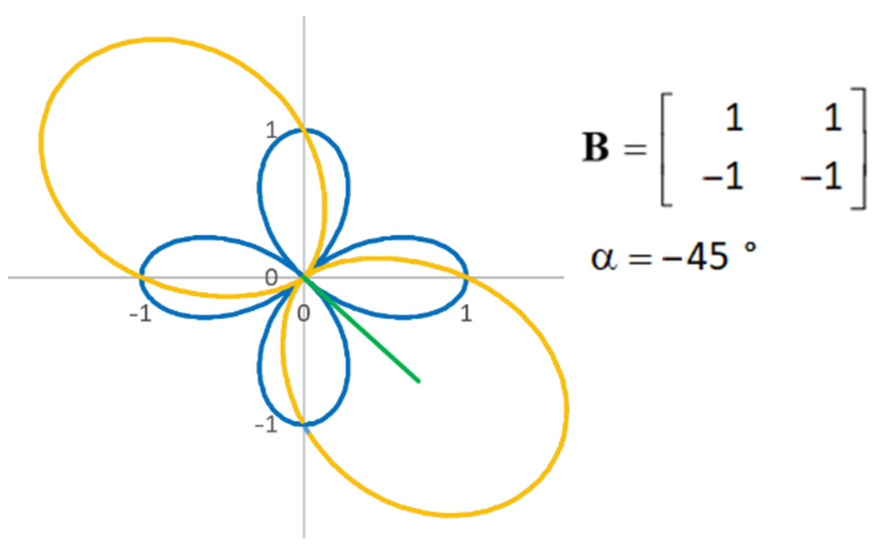
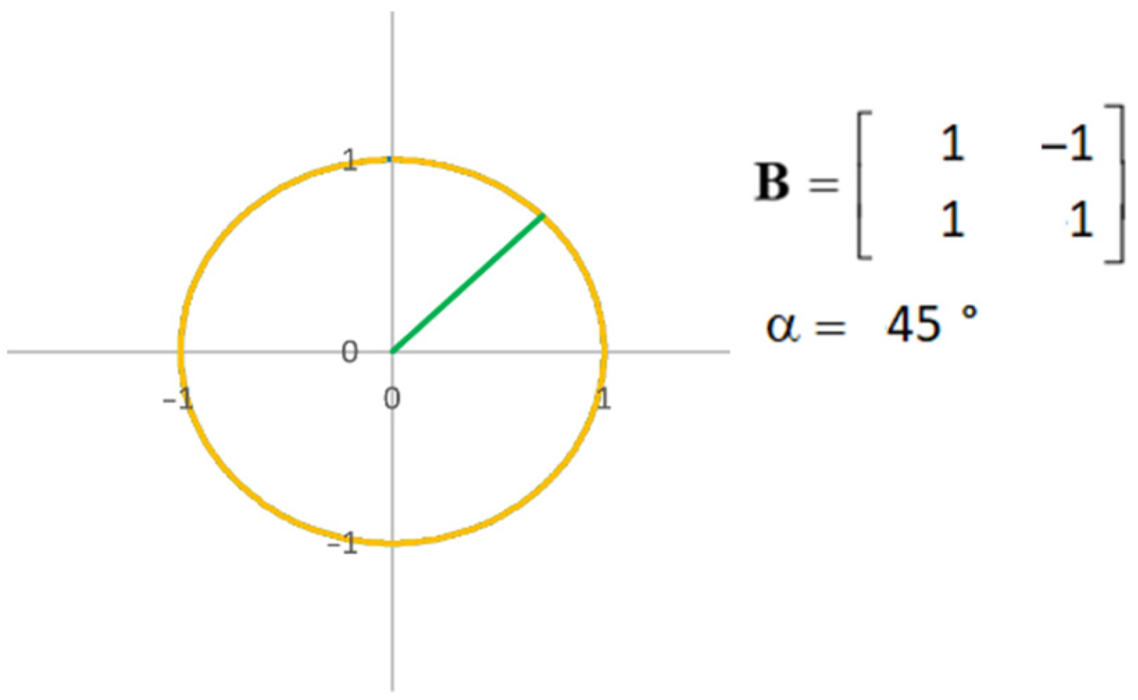
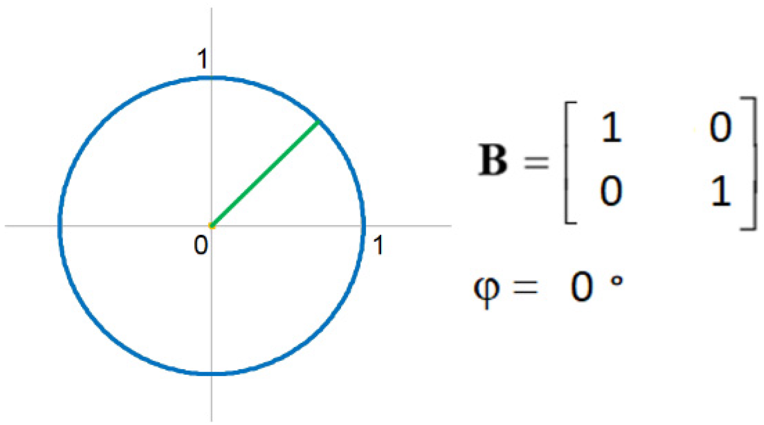
Components of this rotational matrix can be a part of some general tensor. Upon defining the square matrix components, the matrix can be decomposed into symmetric and antisymmetric tensors. Typically, for this tensor, the initial angle always equals . However, with every rotation of the rotational matrix by angle , a new general tensor emerges. Figure 11, Figure 12, Figure 13 and Figure 14 show examples of different tensors corresponding to some of the rotational matrix states.
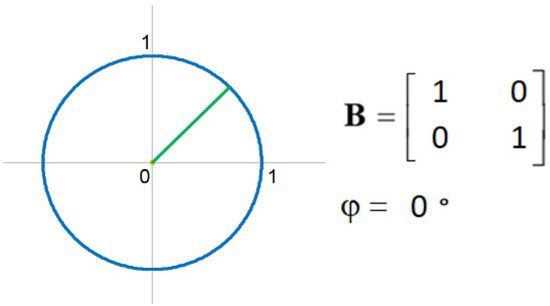
Figure 11.
General tensor for rotational matrix with angle .
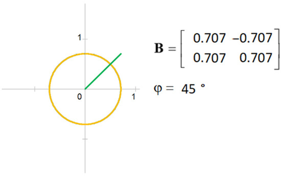
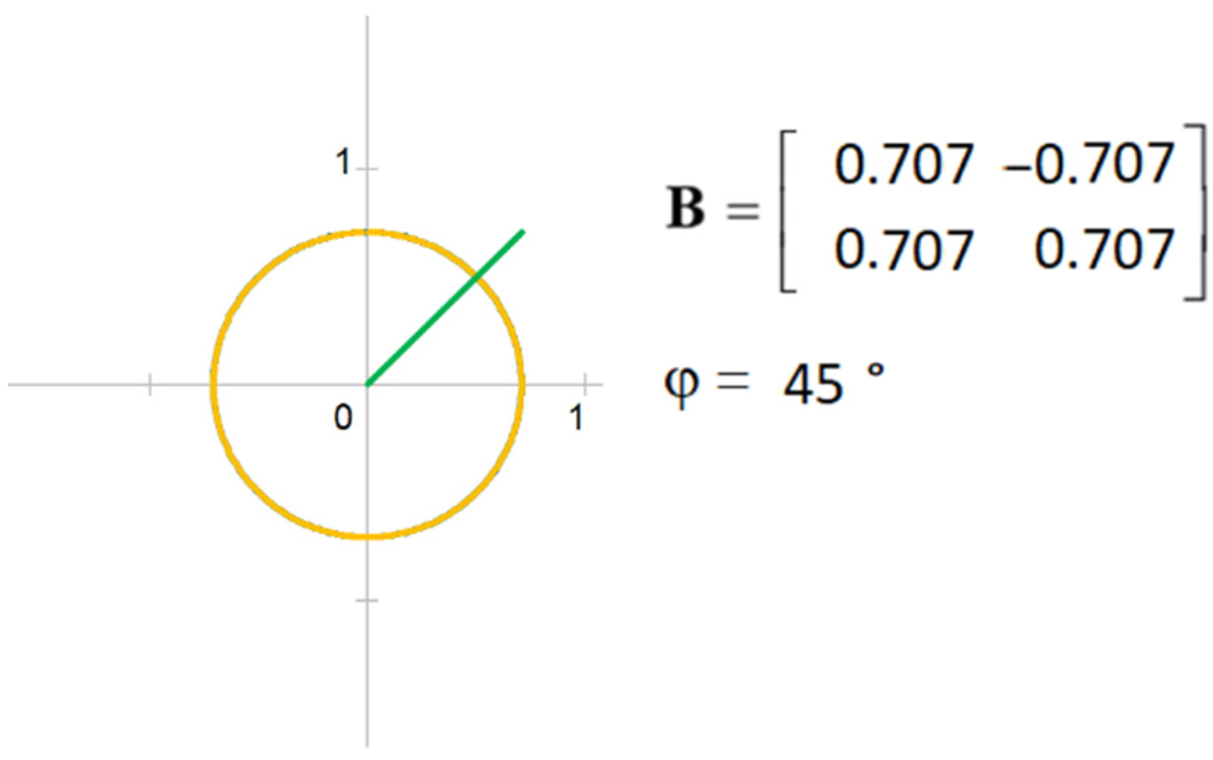
Figure 12.
General tensor for rotational matrix with angle .
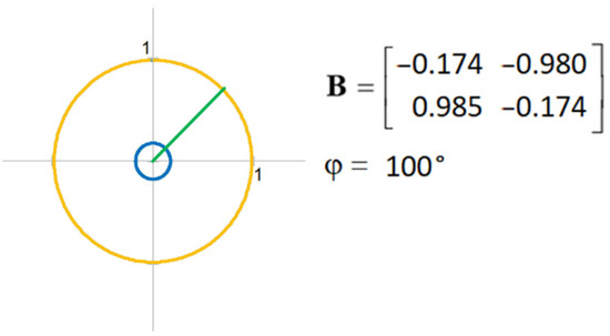
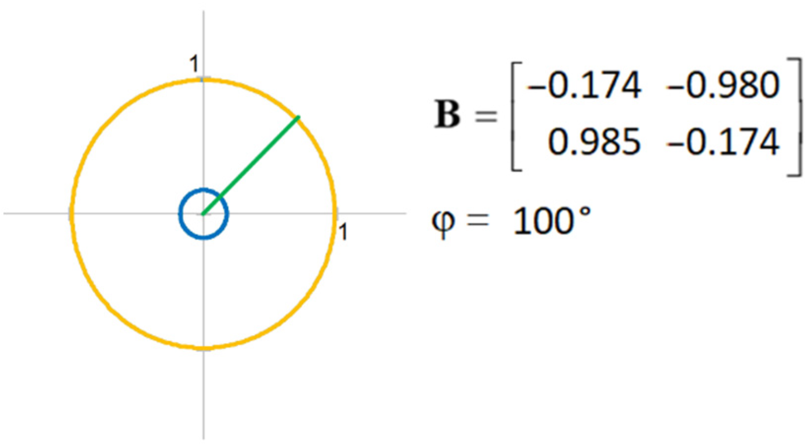
Figure 13.
General tensor for rotational matrix with angle .
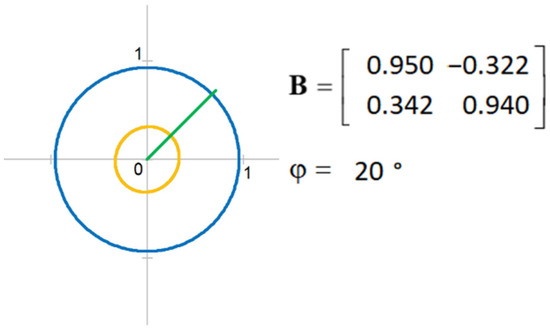
Figure 14.
General tensor for rotational matrix with angle .
As can be seen, in all cases, the tensor shape is made of the diagonal matrix components and , which give rise to two concentric circles.
6. Golden Section in Tensor Visualization
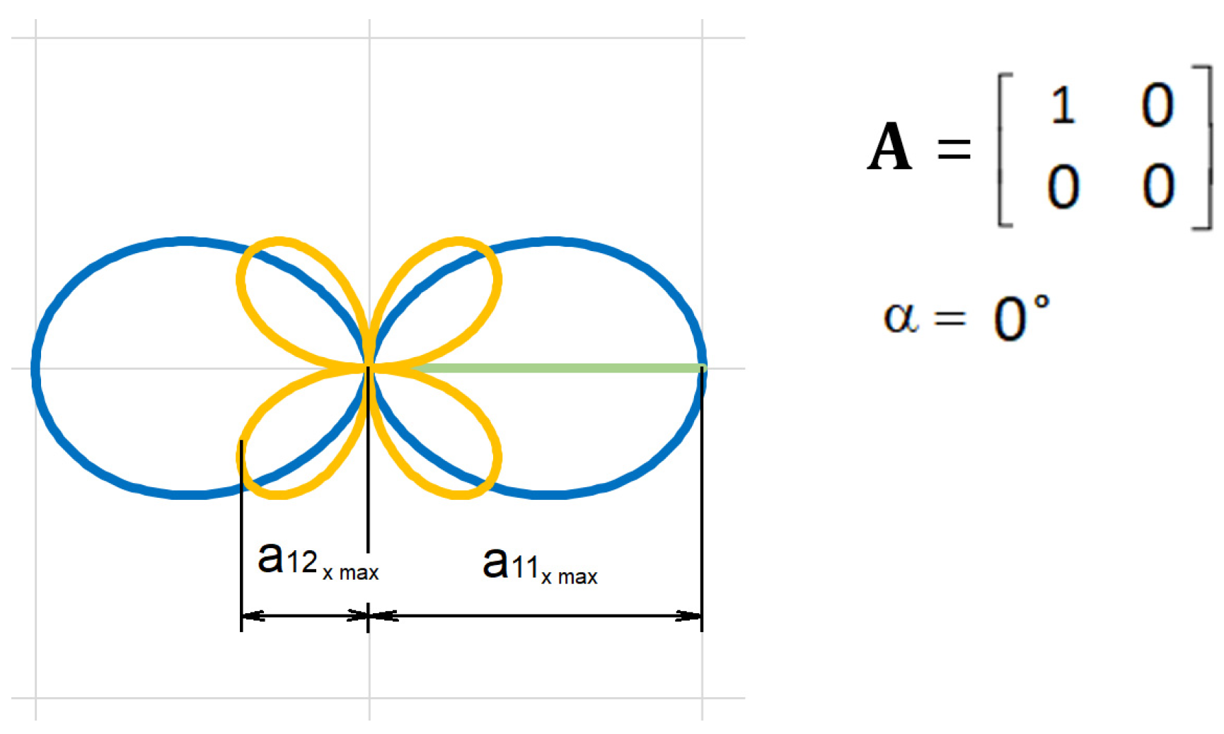
Shape proportions created by diagonal symmetric tensor components depend solely on the angle of the initial vector. With the initial state , the maximum values of tensor component parts in the x-axis direction display the golden section ratio (Figure 15).
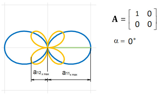
Figure 15.
Symmetric tensor with .
This fundamental relation is introduced without being derived mathematically. It was obtained through measurement. If we view the symmetric tensor as a glyph, the shape of which changes symmetrically, in terms of glyph symmetry, this condition is achieved under a 45° angle.
7. Discussion and Conclusions
Tensors are fundamental building blocks used to describe physical phenomena. In the orthogonal coordinate system, their shape diversity is limited, as shown in Figure 2, Figure 3, Figure 4, Figure 5, Figure 6, Figure 7, Figure 8, Figure 9, Figure 10, Figure 11, Figure 12, Figure 13 and Figure 14. It follows from the analysis that these analytical glyphs are unambiguous in terms of their shape. The analytical calculations presented in Section 4 are also highly likely to hold by analogy for 3D space. A substantial barrier to creating analytical calculations has been the absence of the third invariant in 2D space. In a similar fashion, the fourth tensor invariant for 3D space is also missing. It is necessary to derive the calculations for the symmetrical tensor first, followed by the asymetrical tensor. In addition, the change in the eigenvalues order on the main tensor diagonal is necessary to ensure that solving the equation always yields a real number instead of a complex one. The changed order does not lead to loss of information on tensor properties and the real numbers can be visualized in 3D rendering.
An interesting observation is that the symmetric tensor shape under zero angle of the initial state, as shown in Figure 15, has a proportional relation to the golden section ratio. This is significant because this commonly known principle, abundantly present in organic nature, was found at the heart of the tensor calculation. By means of the constant φ, the symmetric tensor is connected to the complex plane in the same way as the significant constants and . This is, therefore, likely to be a fundamental principle. The golden section ratio can also be encountered in relation to the strength of materials theory [19], as mentioned in the conclusion of an important paper by Michell [27]. These references to the golden section ratio are not limited to the plane only; they can also be found in attempts to describe higher dimensions. A paper dealing with transformations of a Pythagorean-like formula for surfaces immersed in three-dimensional space forming constant sectional curvature in a Riemann sphere examined the first, second, and third fundamental forms of the surface, proving that the immersed surfaces are totally round spheres with Gauss-like curvature φ + c, where φ is the golden ratio [28]. This, too, is a fundamental principle.
This paper’s main contributions are as follows:
- (a)
- A new analytical approach to deriving rank two tensor components in a plane;
- (b)
- Analytic tensor glyph visualization of the rank two tensor in a plane by representing all components in every direction;
- (c)
- Definition of a new tensor invariant that can be added to all dimensions;
- (d)
- Pointing out the golden ratio law present in the representation of a planar tensor with a zero initial angle (as shown in Figure 15).
Tensor glyphs imaging is a progressive and useful method when applied to in-depth analysis of dynamic processes. Currently, only numerical methods for imaging exist, resting on different principles mentioned in the introductory section. Due to computation constraints, some principles are not capable of determining all tensor glyph properties. In analytical calculation, this problem ceases to exist. However, a special transfer system for transforming complex results into the real space had to be used; details of the technique used to that end were given in Section 3.
Author Contributions
Conceptualization, T.S.; methodology, T.S.; resources, T.S.; writing—original draft preparation, T.S.; writing—review and editing, J.S. and J.D.; project administration, J.S. All authors have read and agreed to the published version of the manuscript.
Funding
This work was supported by the Slovak Research and Development Agency under contract no. APVV-18-0413, KEGA 016TUKE-4/2021 and KEGA 063TUKE-4/2021.
Institutional Review Board Statement
Not applicable.
Informed Consent Statement
Not applicable.
Data Availability Statement
Not applicable.
Conflicts of Interest
The authors declare no conflict of interest.
Appendix A
Determining the third invariant .
Let there be the following input equations:
Let us insert the following components (A1) into the equation:
Let us add up the equations:
Let us insert the parameters :
As shown, the third invariant is also linearly independent of other invariants. Nonetheless, a certain form of quadratic dependence does exist between the invariants. We insert the tensor components (A5) into the equation:
Appendix B
Calculating the components of .
Let there be the following input equations:
The input equations shall be adjusted as follows:
Let us determine the product of the components :
Let us express the component :
Component is calculated from the quadratic equation (A27):
References
- Borgo, R.; Kehrer, J.; Chung, D.H.; Maguire, E.; Laramee, R.S.; Hauser, H.; Ward, M.; Chen, M. Glyph-based visualization: Foundations, design guidelines, techniques and applications. In Eurographics State of the Art Reports; The Eurographics Association: Hannover, Germany, 2013; pp. 39–63. [Google Scholar]
- Gerrits, T.; Rössl, C.; Holger Theisel, H. Glyphs for general second-order 2d and 3d tensors. IEEE Trans. Vis. Comput. Graph. 2016, 23, 980–989. [Google Scholar] [CrossRef] [PubMed]
- Sarwar, T.; Ramamohanarao, K.; Zalesky, A. Mapping connectomes with diffusion MRI: Deterministic or probabilistic tractography? Magn. Reson. Med. 2019, 81, 1368–1384. [Google Scholar] [CrossRef] [PubMed]
- Muhammed, A.M.; Aswathi, V. Analysis of Visualization Techniques in Diffusion Tensor Imaging (DTI). In Proceedings of the 2018 Second International Conference on Advances in Electronics, Computers and Communications (ICAECC), Bengaluru, India, 9–10 February 2018. [Google Scholar]
- Kratz, A.; Björn, M.; Hotz, I. A visual approach to analysis of stress tensor fields. In Scientific Visualization: Interactions, Features, Metaphors, 1st ed.; Hagen, H., Ed.; Schloss Dagstuhl—Leibniz-Zentrum für Informatik GmbH: Kaiserslautern, Germany, 2011; Volume 2, pp. 188–211. [Google Scholar]
- Hashash, Y.; Yao, J.; Wotring, D. Glyph and hyperstreamline representation of stress and strain tensors and material constitutive response. Int. J. Numer. Anal. Methods Geomech. 2003, 27, 603–626. [Google Scholar] [CrossRef]
- Schroeder, W.; Martin, K.M.; Lorensen, W. The design and implementation of an object-oriented toolkit for 3D graphics and visualization. In Proceedings of the 7th Annual IEEE Conference on Visualization (Visualization 96), San Francisco, CA, USA, 27 October–1 November 1996. [Google Scholar]
- Delmarcelle, T.; Hesselink, L. Visualizing second-order tensor fields with hyperstreamlines. IEEE Comput. Graph. Appl. 1993, 13, 25–33. [Google Scholar] [CrossRef] [Green Version]
- Zobel, V.; Scheuermann, G. Extremal curves and surfaces in symmetric tensor fields. Visual Comput. 2018, 34, 1427–1442. [Google Scholar] [CrossRef]
- Kindlmann, G. Superquadric tensor glyphs. In Proceedings of the Sixth Joint Eurographics-IEEE TCVG Conference on Visualization, Konstanz, Germany, 19–24 May 2004; pp. 147–154. [Google Scholar]
- Schultz, T.; Kindlmann, G.L. Superquadric glyphs for symmetric second-order tensors. IEEE TVCG 2010, 16, 1595–1604. [Google Scholar] [CrossRef] [PubMed] [Green Version]
- Globus, A.; Levit, C.; Lasinski, T. A tool for visualizing the topology of three-dimensional vector fields. In Proceedings of the the second annual IEEE conference on Visualization, San Diego, CA, USA, 22–25 October 1991; pp. 33–40. [Google Scholar]
- Theisel, H.; Weinkauf, T.; Hege, H.C.; Seidel, H.P. Saddle connectors—An approach to visualizing the topological skeleton of complex 3d vector fields. In Proceedings of the 14th IEEE Visualization, Washington, DC, USA, 22–24 October 2003; pp. 225–232. [Google Scholar]
- Crossno, P.; Rogers, D.H.; Brannon, R.M.; Coblentz, D. Visualization of salt-induced stress perturbations. In Proceedings of the 15th IEEE Visualization Conference, Austin, TX, USA, 10–15 October 2004; pp. 369–376. [Google Scholar]
- Feragen, A.; Fuster, A. Geometries and interpolations for symmetric positive definite matrices. In Modeling, Analysis, and Visualization of Anisotropy, 1st ed.; Schultz, T., Özarslan, E., Hotz, I., Eds.; Springer: Dordrecht, The Netherlands, 2017; pp. 85–113. [Google Scholar]
- Hlawitschka, M.; Scheuermann, G. HOT-lines: Tracking lines in higher order tensor fields. In Proceedings of the 16th IEEE Visualization Conference, Minneapolis, MN, USA, 23–28 October 2005; pp. 27–34. [Google Scholar]
- Healy, D.; Timms, N.E.; Pearce, M.A. The variation and visualisation of elastic anisotropy in rock-forming minerals. Solid Earth 2020, 11, 259–286. [Google Scholar] [CrossRef] [Green Version]
- Lord, N. The moment of inertia of an elliptical wire. Math. Gaz. 2014, 98, 121–125. [Google Scholar] [CrossRef]
- Fleisch, D.A. A Student’s Guide to Vectors and Tensors; Cambridge University Press: Cambridge, UK, 2011; p. 134. [Google Scholar]
- Sharpe, R.W. Differential Geometry: Cartan’s Generalization of Klein’s Erlangen Program; Springer Science & Business Media: New York, NY, USA, 2000; pp. 194–200. [Google Scholar]
- Kline, M. Mathematical Thought from Ancient to Modern Times: Volume 3; Oxford University Press: New York, NY, USA, 1990; pp. 1127–1128. [Google Scholar]
- Lee, J.M. Smooth manifolds. In Introduction to Smooth Manifolds; Springer: New York, NY, USA, 2013; pp. 304–316. [Google Scholar]
- Lang, S. The Tensor Product. In Algebra. Graduate Texts in Mathematics; Springer: New York, NY, USA, 2002; Volume 211, pp. 601–603. [Google Scholar]
- Jeevanjee, N. An Introduction to Tensors and Group Theory for Physicists; Birkhäuser: New York, NY, USA, 2011; pp. 39–54. [Google Scholar]
- Dodson, C.T.J.; Poston, T. Tensor Geometry Springer-Verlag. Grad. Texts Math. 1991, 120, 105–106. [Google Scholar]
- Stejskal, T.; Dovica, M.; Svetlík, J.; Demeč, P.; Hrivniak, L.; Šašala, M. Establishing the Optimal Density of the Michell Truss Members. Materials 2020, 13, 3867. [Google Scholar] [CrossRef] [PubMed]
- Michell, A.G.M. The limits of economy of material in frame-structures. Philos. Mag. 1904, 8, 589–597. [Google Scholar]
- Aydin, M.E.; Mihai, A.A. Note on Surfaces in Space Forms with Pythagorean Fundamental Forms. Mathematics 2020, 8, 444. [Google Scholar] [CrossRef] [Green Version]


Publisher’s Note: MDPI stays neutral with regard to jurisdictional claims in published maps and institutional affiliations. |
© 2022 by the authors. Licensee MDPI, Basel, Switzerland. This article is an open access article distributed under the terms and conditions of the Creative Commons Attribution (CC BY) license (https://creativecommons.org/licenses/by/4.0/).