Abstract
The classification of sound signals can be applied to the fault diagnosis of mechanical systems, such as vehicles. The traditional sound classification technology mainly uses the time-frequency domain characteristics of signals as the basis for identification. This study proposes a technique for visualizing sound signals, and uses artificial neural networks as the basis for signal classification. This feature extraction method mainly uses a principle to convert a time domain signal into a coordinate symmetrized dot pattern, and presents it in the form of snowflakes through signal conversion. To verify the feasibility of this method to classify different noise characteristic signals, the experimental work is divided into two parts, which are the identification of traditional engine vehicle noise and electric motor noise. In sound measurement, we first use the microphone and data acquisition system to measure the noise of different vehicles under the same operating conditions or the operating noise of different electric motors. We then convert the signal in the time domain into a symmetrized dot pattern and establish an acoustic symmetrized dot pattern database, and use a convolutional neural network to identify vehicle types. To achieve a better identification effect, in the process of data analysis, the effect of the time delay coefficient and weighting coefficient on the image identification effect is discussed. The experimental results show that the method can be effectively applied to the identification of traditional engine and electric vehicle classification, and can effectively achieve the purpose of sound signal classification.
1. Introduction
Traditional sound identification often relies on the differences in sound characteristics perceived by the human ears. Advanced signal processing analysis methods, Fourier transform and wavelet transform for the time domain signal, can be used to recognize sound features as the basis for recognition. However, the Fourier-transformed frequency domain map cannot simultaneously show the sound characteristics in the time domain and easily distinguish differences in sound characteristics based on the human ear. The original acoustic signal is converted in this study using a symmetrical point map. The acoustic signal is then visually processed. The acoustic signal is identified using the convolutional neural network. This study will first use convolutional neural network recognition from traditional engine vehicle noise symmetry point patterns, and then extend the research to electric motor noise recognition.
In 1986, Pickover [1] proposed the sound symmetrized dot pattern (SDP) concept and formula, which successfully visualized sound characteristics. In particular, Gaussian noise and white noise have little difference whether shown on a power diagram or spectrum diagram, making it difficult to distinguish between the two. However, there is a significant difference between Gaussian noise and white noise represented on the sound symmetric point diagram. In 1997, Derosier et al. [2] proposed a study on the SDP gain coefficient of the mechanical characteristics of food products, and discussed the influence of the gain coefficient on the pattern. In 2000, Shibata et al. [3] put forward rotating machinery fault diagnosis through sound signal visualization. In 2004, Dudkowska and Makowiec [4] used the artificial symmetrized pattern (AIP) to observe heart rate characteristics, and used AIP to analyze the health of the heart. Wu and Chuang [5] used acoustic and vibration signal visual dot patterns to diagnose internal combustion engine faults. It was shown that the sound SDP can show vehicle noise, and different internal combustion engine failures can be observed. The sound SDP can present internal combustion engine failure characteristics as of 2005. In 2011, Cheng et al. used a wavelet space filter and symmetry point diagram to diagnose abnormal internal combustion engine noises [6]. In 2014, Tomasz [7] used frequency domain diagrams to analyze the problem points spark ignition (SI) engines under fixed and non-fixed conditions. Wang [8] proposed using sound symmetry point maps with a pattern matching system as a vehicle type identification method. However, due to the rapid development of internet technology and improvements in computer equipment efficiency in recent years, deep learning has been used to introduce many sophisticated picture classification methods. A cat’s brain wave response was observed in cat vision system research, as proposed by Hubel and Wiesel in 1962. Their research results on neuron output and input as well as cell response were proposed [9]. Their research laid a foundation for deep learning development.
A self-organizing neural network model was proposed by Kunihiko in 1980 [10]. The model in this article is the theoretical basis of imitation, which can be said to be the beginning of the convolutional layer and pooling layer of CNN. Brain neuroscience results were converted into computer and model simulations commonly used in convolutional neural networks (CNN) proposed. Alex et al. [11] applied the convolutional neural network to machine vision competition. The convolutional neural network exhibited excellent picture recognition performance in 2012, and a regularization method called drop out was proposed. In 2016, Vedaldi [12] proposed that MatConvNet is a CNN for MATLAB. It can quickly design the architecture of CNN and support high-performance computing on CUP and GPU. In 2018, Konovalenko et al. [13] proposed using CNN to study titanium alloy fractured surfaces, diagnose metal sections, and determine the fracture time for analysis. It can be confirmed that CNN is used to classify images more accurately, and the manual adjustment of parameters can be a reduced quantity. In 2018, Abiyev and Ma’aitah [14] proposed a deep convolutional neural network for chest disease detection. X-ray film was used for deep learning classification, which can effectively diagnose chest diseases. From this article, we can understand the system architecture of CNN and design principles. In 2018, Vinken et al. [15] used deep convolutional neural networks to study regular and irregular shapes represented by monkey inferior temporal neurons and human judgments. To identify natural images of objects, they used CNN to compare training and untraining. In 2017 Jain et al. [16] proposed using optical character recognition (OCR) to identify vehicle systems. Using different methods for identifying vehicles, scanned images can be coded to identify vehicles. Zhang and Jiang [17] proposed neural network-based road vehicle type identification in 2009. After preprocessing the vehicle image, the image features are extracted, and the BP neural network is trained and tested for image classification. In 2015, Zeng et al. [18] proposed using symmetrical polar coordinates to identify diesel engine fault detection. It was shown in the article that the SDP spacing angle should not be too dense, because too dense may lead to signal overlap in using SDP with an internal angle of 60°. In 2019, González et al. [19] used SDP to observe vehicle air-conditioning systems, converted the vibration signals of different faults, converted time waveforms into SDP, and unified the SDP parameters used in rotating machinery vibration analysis. In 2019, Nilwong et al. [20] used a single convolutional neural network (CNN) to determine the position and locate the compass direction from the entire image. The research method pointed out that the image position can be confirmed by training through the CNN network. The accuracy of positioning in an outdoor environment. In 2020, due to the improvement of energy structure, Yalong et al. [21] were unable to adjust wind turbines for natural wind power in the past. They established a historical wind power database using CNN and collected long-term weather data to estimate short-term wind power using the wind power curve. In 2021, Pham et al. [22] used CNN to determine the type of fault classification in the bearing, because the bearing is a component that supports rotation. When the working state of the bearing and its fault state can be classified accurately, it can effectively solve the complex fault diagnosis problem. In 2021, Colantonio et al. [23] discovered that in lathe cutting operations, tool wear is inevitable, but due to tool wear, the probability of producing defective products increases. Through various deep learning calculations, the framework of the tool status in stable turning can be monitored. In 2021, Fentaye et al. [24] set up different failure scenarios of aircraft engines through step-by-step detection, and distinguished and accurately classified various failures through deep learning. In 2022, Zou et al. [25] used CNN to deal with the problem of the inability to extract rice features in general image recognition, and successfully used CNN to complete a number of rice calculations.
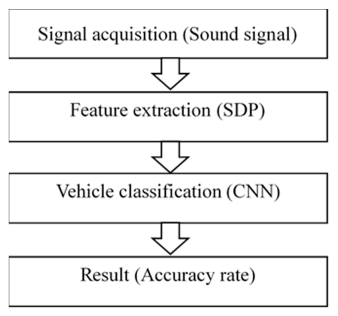
Because CNN works have excellent image classification and image recognition performance, SDP and convolutional neural networks will be used to identify vehicle types. Compared with traditional methods to distinguish pictures, CNN can more efficiently identify vehicle types. The main structure of this research is divided into three parts: data acquisition, visual processing of sound signals, and vehicle noise symmetrical points identification. The signal is first converted into a sound SDP. The vehicle noise sound SDP is then labeled and the convolutional neural network operation is used to identify the vehicle type sound symmetrical point pattern. The various noise coefficients effects on the SDP vehicle noise on the identified vehicle types are discussed. An attempt is made to find the optimal gain coefficient of the vehicle noise symmetry point diagram to obtain the best vehicle type identification result.
2. Materials and Methods
2.1. Symmetrized Dot Pattern Principle
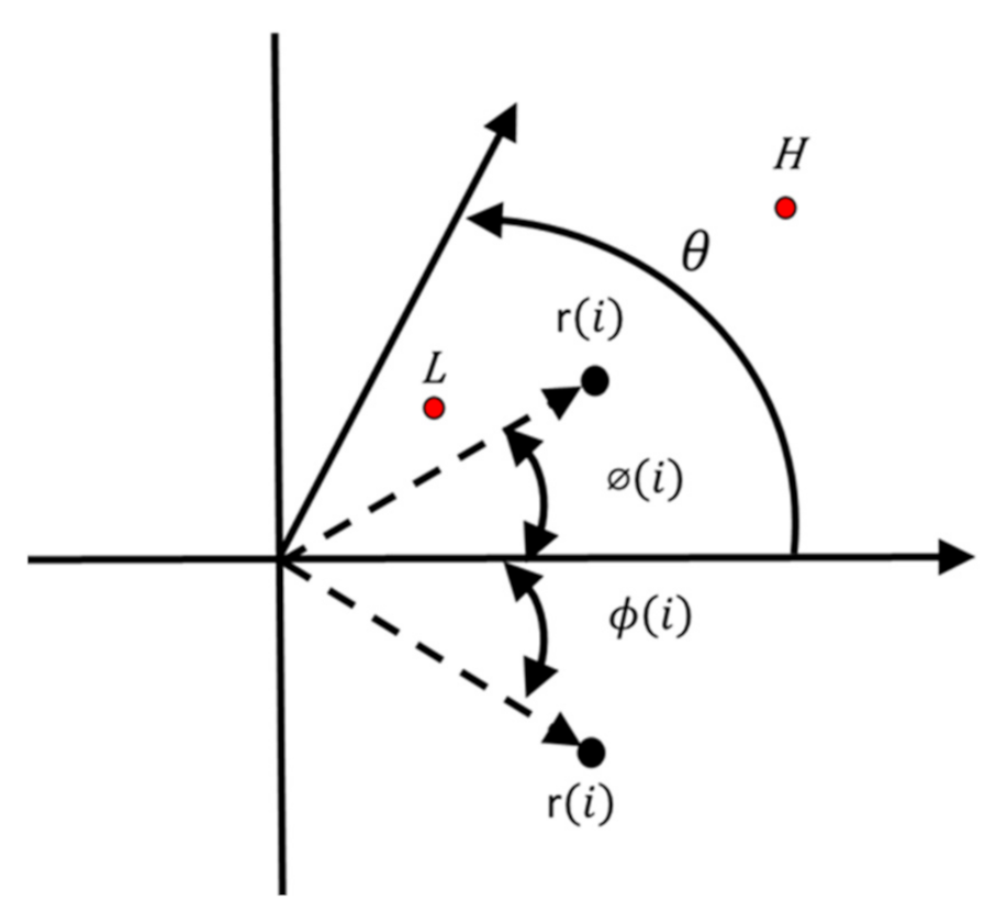
SDP is used to represent sound signal characteristics. The symmetrized dot pattern is used to visualize the sound or vibration signal. Polar coordinates are used to project the time domain data onto the coordinates. The point pattern is used to show the signal characteristics to form a picture that changes with time, forming a symmetrical snowflake-like figure. The sound signals of various conditions are presented with symmetrized dot patterns. This method presents the differences in sound wave and vibration signals [19]. Figure 1 shows the sound symmetry dot pattern principles, R(i) represents point i in the signal, the radius from the origin of the coordinates of that point. ∅(i) and ϕ(i) are the setting angles of each point on the sound symmetrical dot pattern, ∅(i) is a positive angle, and ϕ(i) is a negative angle.

Figure 1.
Symmetrized dot pattern principle.
In this study, point of sound symmetry is used to present acoustic signal characteristics. The sound symmetrized dot pattern visualizes the sound or vibration signal. Polar coordinates are used to project the time domain data onto the coordinates. The point chart is used to show the signal characteristics, forming a picture that changes with time. The sound signals of a symmetrical snowflake-like figure in various experimental conditions are presented in this study. This method can present the differences in sound waves and vibration signals.
In Equation (1) the sound symmetrized dot pattern, F(t) represents the time axis signal. When the time axis signal is F(t + n), the time of the next signal point is t + n. Fixed sampling time n pairs of discontinuous signals F(n) to the polar coordinates represented using the following equation:
F(i) represents a certain sound or vibration signal, H is the maximum signal value F(i), L is the minimum signal value F(i), θ is the angle of rotation from the starting line, and t is the time delay coefficient, ζ is a weighting coefficient. It can be seen that Equation (2) represents the SDP graph distributed from the positive start line, while Equation (3) represents the SDP graph distributed from the negative start line.
The symmetric dot pattern algorithm is used to draw the amplitude of each point in a standard time voltage signal on polar coordinates and present it as a visual pattern. Because the value of each point on the time signal will determine the radius of the point falling on the coordinates, and the connection between each point on the time signal will be expressed in polar coordinates according to the set angle and formed according to different time signal characteristics.
The symmetrized dot pattern will also be different. Figure 2 presents the SDP of various signals. When inputting the signal, the F(n) range will be normalized first. From the data, it can be observed that the H and L values of vehicle noise of the same type are similar, so the symmetrized dot pattern characteristics can be expressed. In the symmetrized dot pattern, the larger time delay coefficient t will make the graph appear more divergent. When the time delay coefficient is larger, each point in the signal is lengthened, and the graph will become wider as shown in Figure 3. When the time delay coefficient t is 1, 2, 3, 5, 10, can see the time delay coefficient t effect on the symmetrized dot pattern. Equation (4) is a positive angle when 360° and Equation (5) is a negative angle equation.
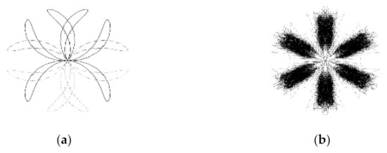
Figure 2.
Signal symmetrized dot pattern (a) 500 Hz sine wave; (b) Random noise.

Figure 3.
SDP of sin waveform (a) SDP figure in various time delay coefficient (t: 1 to 10); (b) SDP figure in various gain coefficient (ζ: 10 to 100).
In addition, in the symmetrized dot pattern, both the weighting coefficient and weighting coefficient ζ have important impact on the symmetrized dot pattern. As shown in Figure 3, the weighting coefficient ζ is larger, the amount of deformation in the graph increases. At 10, 20, 30, 40, and 50, it can be seen that the graph becomes more curved. In addition, in the s symmetrized dot pattern, both of the weighting coefficient and weighting coefficient ζ are important impact on the symmetrized dot pattern. The weighting coefficient ζ is larger, the amount of deformation in the graph increases. At 10, 20, 30, 40, and 50, it can be seen that the graph becomes more curved.
Equation (6) is a positive angle calculation, after the SDP signal is input, the signal is projected onto the polar coordinates, this the signal of the time is the angle of the signal in the counterclockwise direction at 360°, and Equation (7) is a negative angle calculation, after inputting the SDP signal, the signal is projected on the polar coordinates, the signal at this time is the signal is clockwise at 360°.
2.2. Principle of Convolutional Neural Network
Convolutional neural networks are composed of one or more convolutional layers, pooling layers, and fully connected layers. CNN is often used in image and speech recognition. In the study of the cat’s visual system proposed by Hubel and Wiesel in 1962 [9], they mention the local perceptual field, in which neurons can extract certain basic visual features that will be used by higher-level neurons. Product-type neural networks also use the convolutional layer to extract features and performance down sampling through the pooling layer. In the field of category classification, because the convolutional neural network avoids the complicated pre-processing of the picture, the original picture can be used directly as input data in CNN.
In 2012, Krizhevesky et al. [11] applied CNN to competitions in the field of machine vision, which also highlighted the excellent performance of convolutional neural networks in image recognition. Mariana and Tudor [26] sed NN to recognize expressions after occluding part of the face in 2019. Rekowski et al. [27] used CNN to identify forest tree species and used hybrid integration to classify. Down sampling is done through the pooling layer to reduce calculations. is the calculation formula of the convolutional layer, z represents the z plane of the previous level, l represents the number of layers, j represents the j feature plane of the convolution, which is composed of neurons, and represents the selection output. The set of pictures, when z ∈ means that the j layer in the convolution layer belongs to multiple planes of the previous layer, it can be seen that when l − 1 represents the previous layer in this convolution layer, put the i number in the upper layer of the convolution layer is input to the convolution layer, is the weight of the z plane in the layer above the convolution layer and the j feature plane in the convolution layer, and is the j feature plane in the convolution layer. The additional offset parameters are obtained by performing convolution operations on the convolution kernel and the relevant feature plane weights, and the offset parameters are also included [23]. The convolution calculation formula is shown in Equation (8).
In the process of convolutional layer calculation, considering the feature value of the input picture, we can use the function to maintain the feature, and in this study, we chose to use the ReLU function, because the characteristics of this function can keep the input value can be positive, but can slow the gradient. The problem of disappearing or avoiding gradient explosion can also reduce the amount of calculation. In the ReLU formula, the negative value is reset to zero. In Equation (9), x is the output of the previous neural network [10].
In the calculation process of CNN, add Local Response Normalization (LRN), because in the calculation of neural networks, in order to improve accuracy, with LRN will have a better suppression effect. Alex et al. proposed image classification with deep convolutional neural networks [10]. When using local response normalization, the results after the output of the pooling layer can be activated, and this method can make the response larger. In addition, on the contrary, suppressing the small value of the response, to achieve the effect of suppression, can make the model have better adaptability. The calculation formula of LRN is introduced below. a represents the result after the output of the pooling layer, which will be the result of including batches, image length, image width, and the number of neurons passing through. Equation (10) represents the principle calculation of LRN. Containing four kinds of data, is expressed in the positions of these four data output structure, h is at the h kernel at position (x, y), the parameter k is the addition in the denominator, α is the scaling parameter, the size selected by n/2, and β is the exponential term, K, α, n/2, β are self-defined parameters.
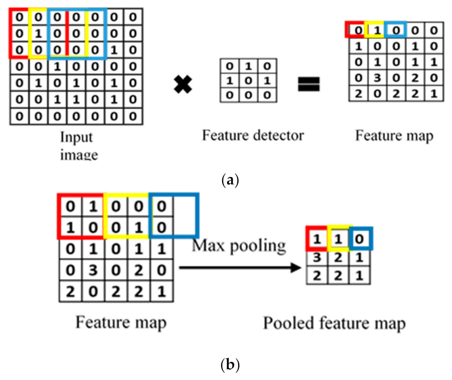
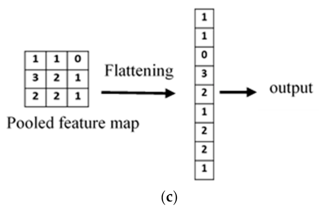
Through the convolution layer operation effect, just as using filters for pictures, we can extract the features of a picture. As shown in Figure 4, Figure 5 and Figure 6, the convolution kernel in the figure is a 3 × 3 matrix, which moves from left to right, from top to bottom, and sets the step when it is 1; the convolution kernel will be moved and multiplied by the feature matrix. The results will be added to the corresponding position, and the final output result will form a feature map. The pooling layer uses maximum pool sampling. It uses a non-linear sampling method to obtain image features through the convolution layer and uses these features to classify. When these features are obtained for analysis, they often generate a very large number of calculations. When acquiring features, a sampling method is performed to extract the maximum feature values to reduce the amount of data, taking the 2 × 2 pooling kernel and the moving step as 2 as an example, it can be seen that after the pooling layer operation, the maximum feature value will be left, and the parameters required for the next layer operation have been reduced. The fully connected layer is a flattened connection of the multi-layer convolutional layer and pooling layer results. The last feature map layer and the last feature map value is connected for image classification tasks.
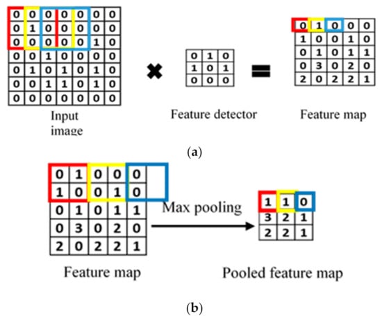

Figure 4.
CNN structure (a) Convolutional layer; (b) Pooling layer; (c) Fully connected layer.
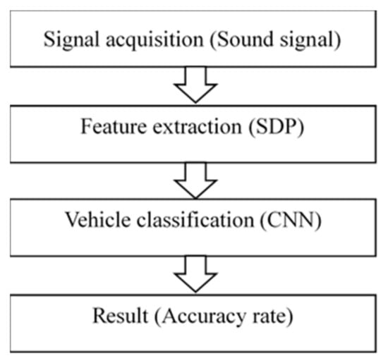
Figure 5.
Vehicle identification flow chart.

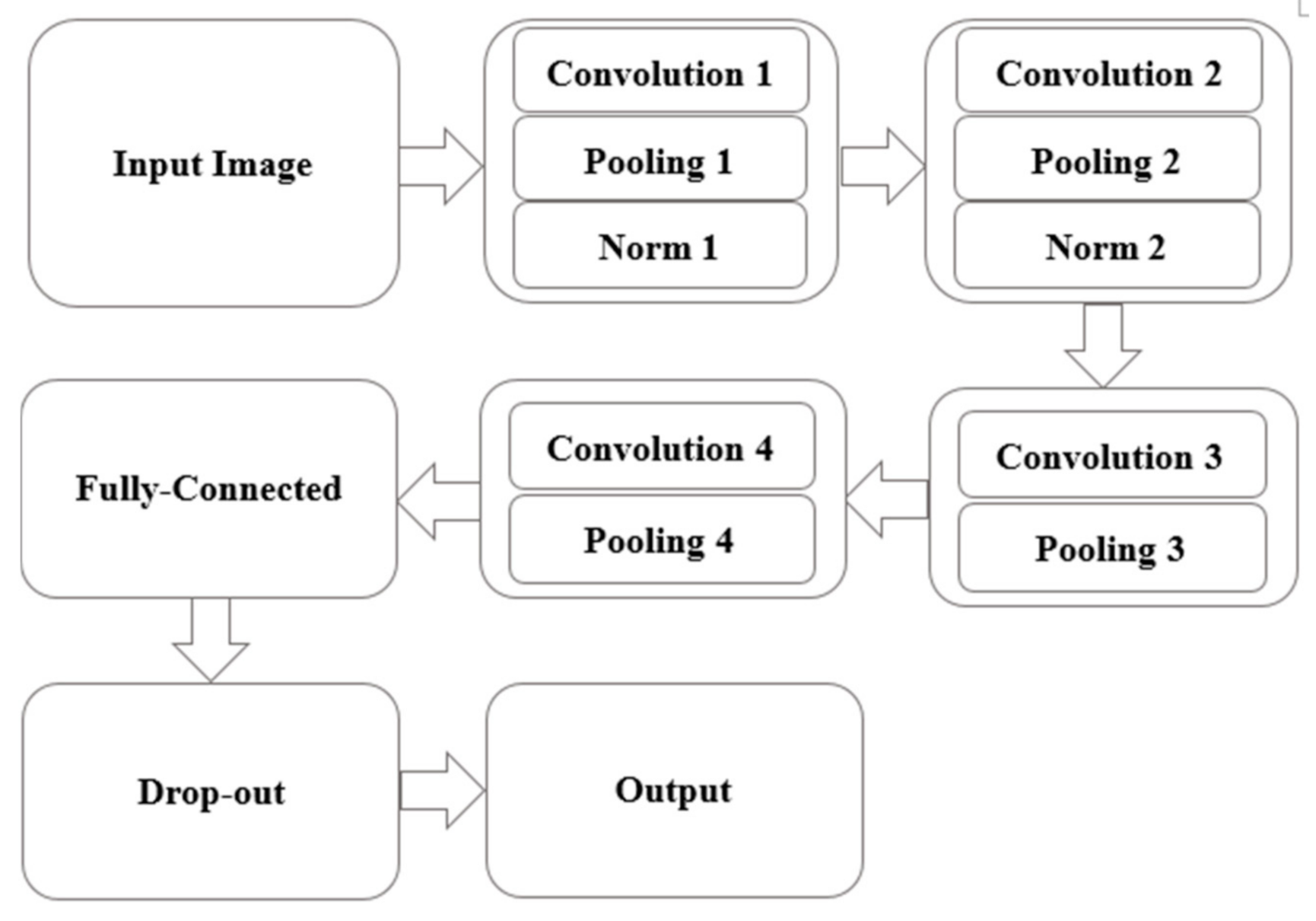
Figure 6.
Convolutional neural network model.
3. Implementation and Experimental Works of Vehicle Classification
3.1. Experimental Work and Data Measurement
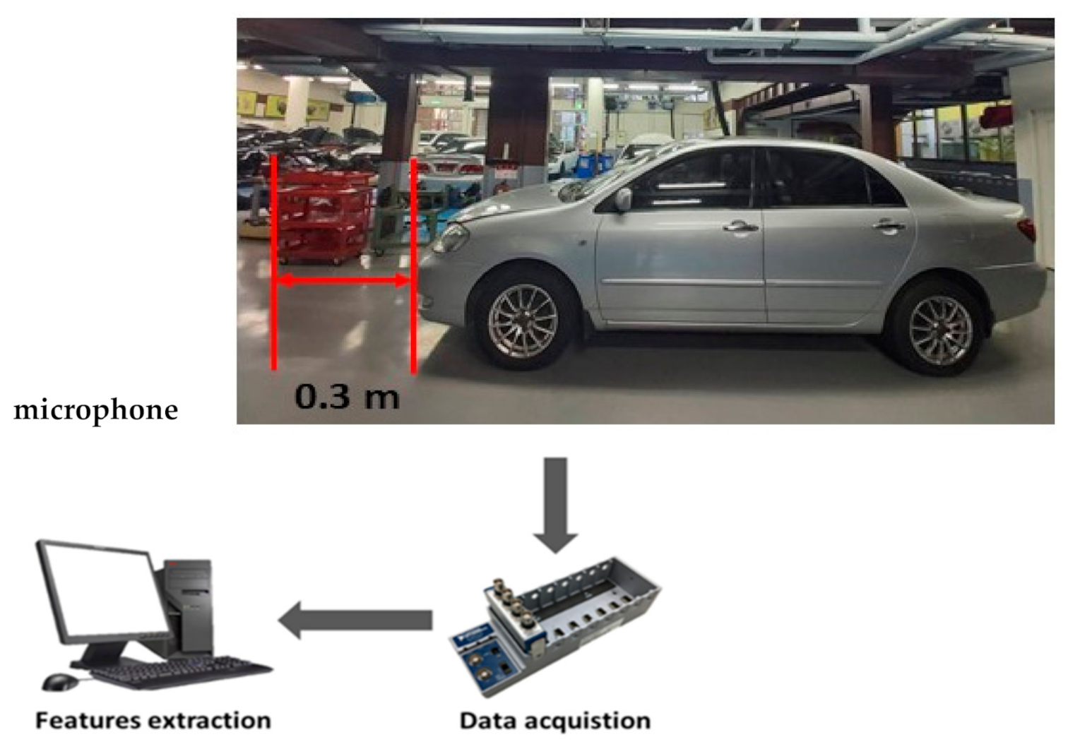
This study will identify vehicle types using different SDP noises. The vehicle identification process is shown in Figure 5. The data acquisition equipment includes microphone (PCB 426E01, PCB Piezotronics, New York, NY, USA), data acquisition system (NI-6024E, National Instruments, Austin, TX, USA), data acquisition card (NI-9233, National Instruments, Austin, TX, USA), notebook computer (ASUS, ASUS Technology, Taiwan) and five vehicles. The vehicle specifications are summarized in Table 1. A microphone was installed 0.3 m in front of the engine. The vehicle speed was maintained at 750 rpm. A data acquisition system and microphone were used to record the engine noise. Labview software (National Instruments, Austin, TX, USA) was used for engine acoustic signal processing. The sampling frequency is set at 2.5 kHz, sampling time is 10 s, has 25,000 points of amplitude data, 30 samples of each vehicle type, and a total of 150 data. This study will explore the vehicle acoustic SDP distribution. And the SDP coefficient ratio effect on picture recognition. Parameter research was conducted on the SDP of various vehicle types to explore the SDP parameter effect on the picture recognition rate. The experimental setup and process of test are shown in Figure 7.

Table 1.
Specification of traditional vehicles in the experiment.

Figure 7.
Experimental setup and process of test.
3.2. Acoustic Signal Processing Using Symmetrized Dot Pattern
- The vehicle noise obtained from the data acquisition system has a total of 25,000 points for each data. The time domain vehicle noise signals are converted into a symmetrical point diagram. The data are presented as an SDP, with a symmetrical point plot drawn for each proportion. Each point in the data will be calculated according to Equations (2) and (3), projected into polar coordinate diagrams, and symmetrical point diagrams of each proportional gain coefficient will be drawn. The sound change symmetrical point diagram changes according to the gain coefficient proportion. When the time delay coefficient increases, the overlapping points in the pictures spread out and the lines become obvious when the weighting coefficient is added as a change condition. Different proportions will have different characteristics. After converting the signal into a picture, the picture will be output in 128 × 128 size.
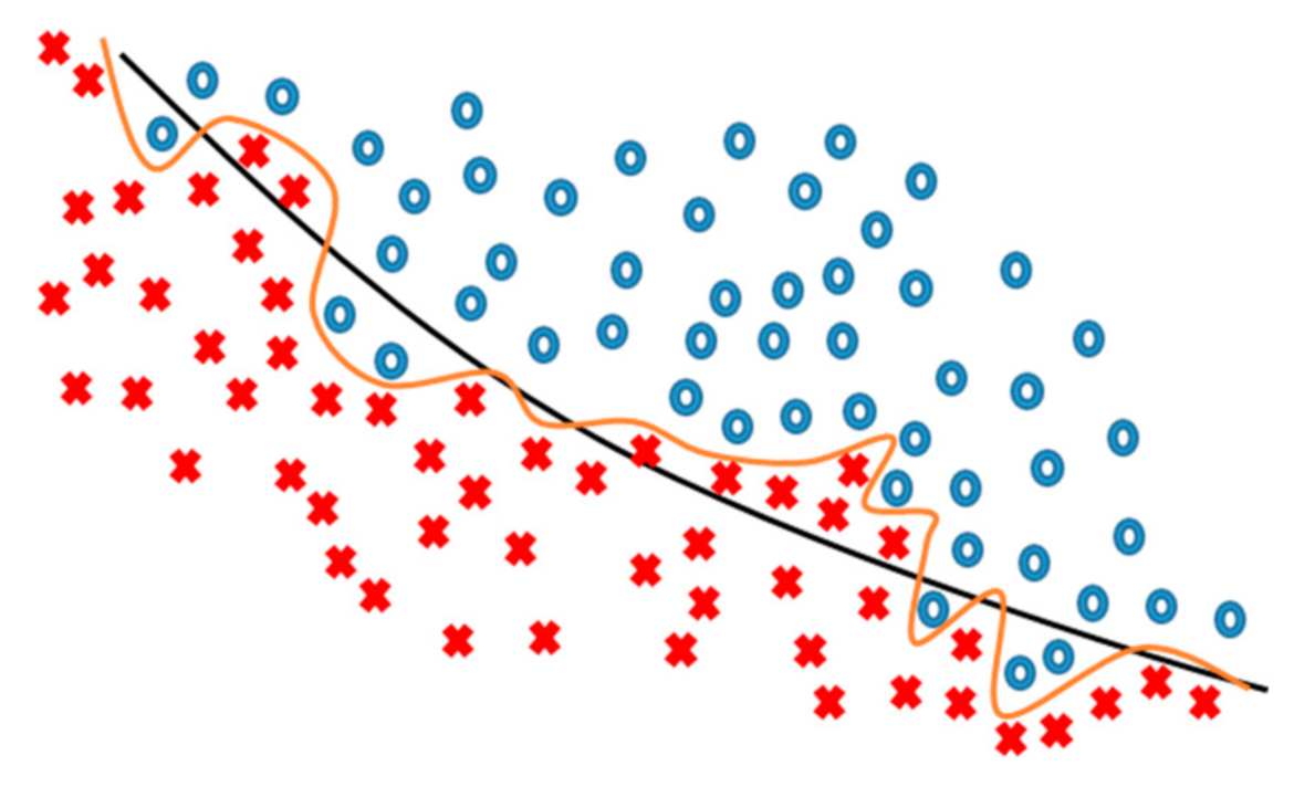
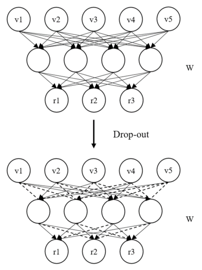
- The Python tensor flow environment was developed by Google and used in this research. Because it supports the programming language C, it is a deep learning environment with a high degree of attention. It is not limited to the deep learning multiple uses and it has reinforced learning and other algorithms. Its ability to run across platforms is strong and can be used and referenced, but the disadvantage is that it runs slower than other environments. The main convolutional neural network architecture is shown in Figure 6, consisting of seven blocks, with four convolutional layers and four pooling layers, finally leading to a fully connected layer. The drop out layer is added to deal with the overfitting the model problem because it avoids relying too highly on sample data during the training process, resulting in an image error value that will not be taken into account during testing. Adding the drop out layer can produce a better fitting effect. The main issue is that when the model parameters are too many and there are too few samples, it is easy to produce overfitting. As showed in Figure 8, in each training batch, some nodes are randomly ignored, so that the neuron will not depend too much on some local features as shown in Figure 9.
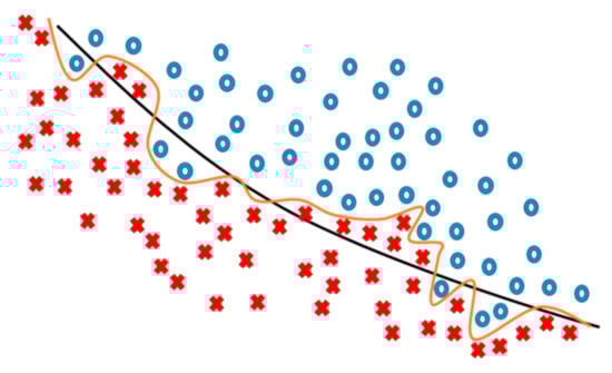 Figure 8. The overfitting principle.
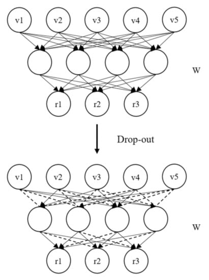 Figure 9. The drop out principle is that the connected neurons are randomly selected and disconnected, eliminating adaptability between neurons during training.
3.3. Experimental Results and Discussion
- The time delay coefficient and weighting coefficient influence on the image recognition effect is researched in this study. First of all, this study completed sound symmetry point mapping of the noise from each vehicle, as shown in Figure 10 and Figure 11. It can be observed that when the gain coefficient changes, it has a great impact on the pattern shape. This study will be focused on understanding the gain factor ratio effect in the proposed system. It can be seen that when the time delay coefficient is increased, the pattern characteristics become obvious. In this study, 60° is used as the interval, and a symmetrical point diagram can be seen, showing a six-petal snowflake shape. The shape of the pattern will be affected by the weighting and time delay coefficients.
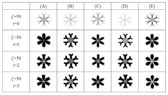 Figure 10. SDP figures in weighting coefficient 50 and time delay coefficient 0 to 3 for five different cars.
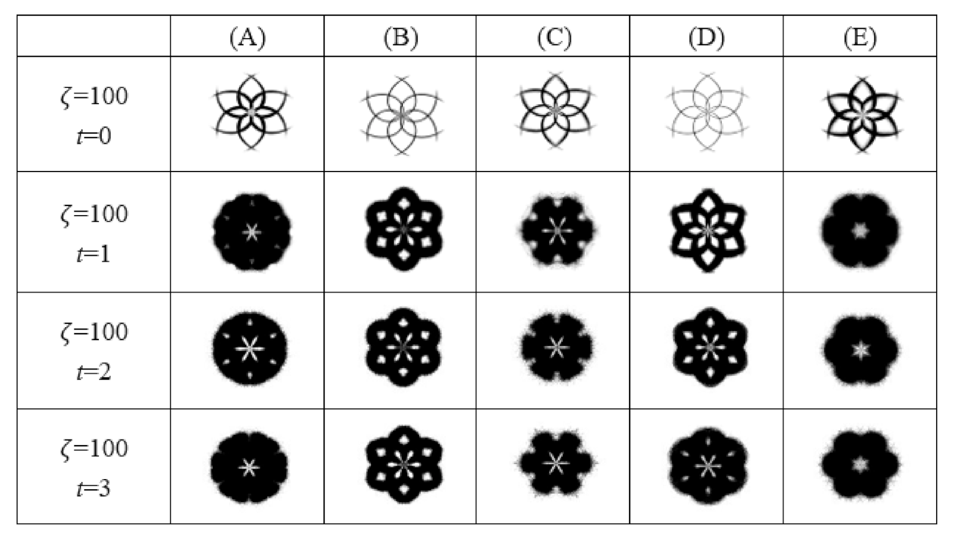
 Figure 11. SDP figures in weighting coefficient 100 and time delay coefficient 0 to 3 for five different cars.
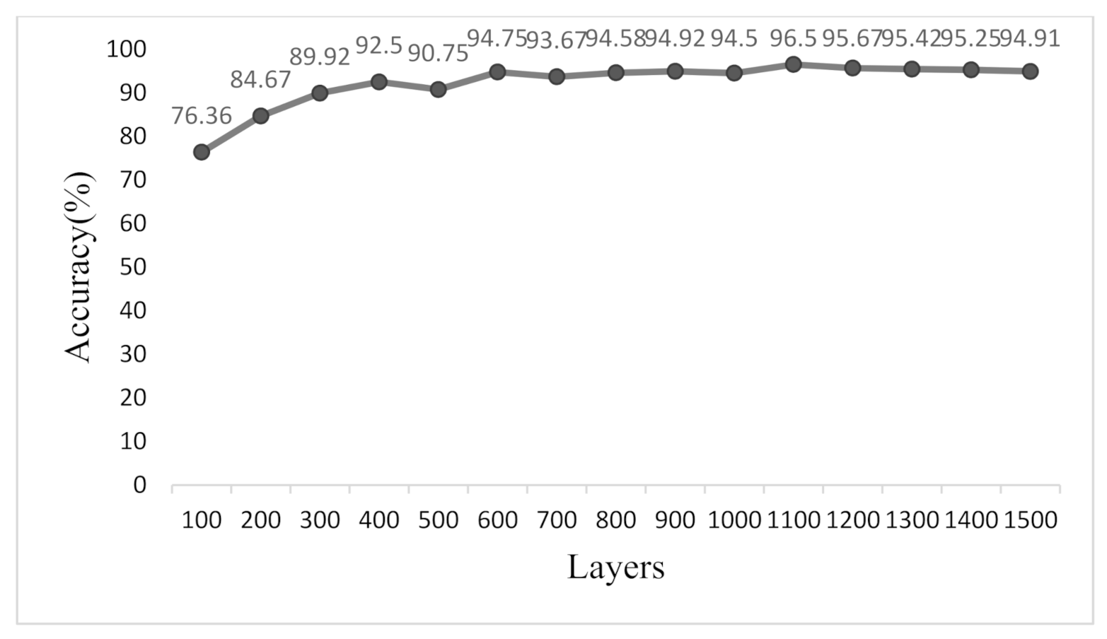
 - When using convolutional neural networks for training and identification, it can be found that the weighting coefficients and time delay coefficients in the symmetric point diagram of noise have an important impact on the recognition of using convolutional neural networks. Therefore, this study attempts to perform an exploration of related variables. First, we try to understand the number of iterative layers effect on the convolutional nerves on the recognition rate. In the data analysis and identification process, when the number of iteration layer changes, it has a significant impact on the overall identification rate. In the experiment, the experimental results are presented with the change of the coefficients, which are in three resulting graphs, which are the identification results on the number of convolutional neural iteration layers, time coefficients, and weighting coefficients. The result is shown in Figure 12, demonstrating that the identification rate can be significantly increased when the number of iterative layers is increased. When the number of iterative layers is higher than 600, the average identification rate can reach about 95%. With the increase in the number of iterations, the recognition rate stabilized, and the effect is not obvious. When drawing a point-symmetric graph, the time delay coefficient also significantly affects the results of the graph. We first set t to vary from 0–3, and explore the coefficient time delay effect on the overall recognition rate. From the results in the figures, it can be observed that there are obvious differences between the different models between 1–3. From the results compiled in Figure 13, it can be shown that when the time delay coefficient is between 1–3, the recognition rate is between 94 and 95%, and the difference is not too obvious. Among them, when time delay coefficient is 2, the average recognition rate is better a little.
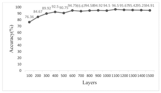 Figure 12. Recognition rates of different iterative layers.
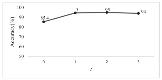 Figure 13. Recognition rates of different time delay coefficients.
 - In addition, we also tried to understand the weighting coefficient ζ influence on the recognition rate. When drawing a point-symmetrical diagram, the weighting coefficient was changed from 10 to 100, and the effect on the average recognition rate was discussed. The results are shown in Figure 14. It shows that when the weighting coefficients ζ are 10, 20, and 40, the average recognition effect is below 90%, and the remaining weighting coefficients can reach more than 90%. Among them, the recognition is the best when the weighting coefficient is 100, and the weighting coefficient ζ is 50. It can reach an average recognition result of more than 95%. This study highlights the possibility of engine signal classification and fault diagnosis when the vehicle is stationary. Although its sound characteristics are somewhat different from the actual driving conditions, the related technology should be applicable to the actual driving conditions. The condition will be applied in other application of electrical vehicle classification.
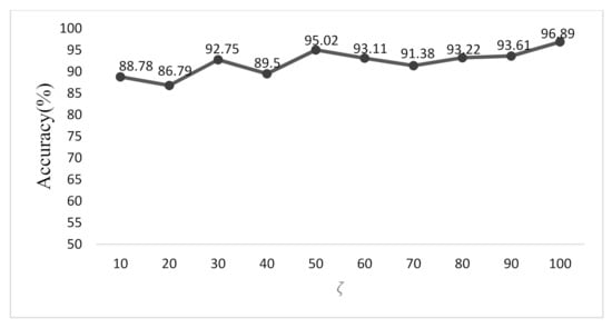 Figure 14. Recognition rates of different weighting coefficients.
4. Discussion
4.1. Electrical Vehicle Experimental Work
The identification results on traditional vehicles showed that the convolutional neural network can effectively identify vehicle noise SDP maps. In another application, the present approach will be used for classifying four electric vehicle motors in electric vehicles experimental samples are brushed toothed motor, brushless toothless motors, brushless toothless motors, and on-board electric vehicle motors. The motor noise is recorded at 200 rpm. In the same way, Labview is used to convert the motor noise signal into a digital signal and processed on the computer. The sampling frequency is 2.5 kHz, the sampling time is 10 seconds, each piece of data is also 25,000 points of amplitude data, and the number of samples for each motor is 30. The experimental process is the same as the previous experiment for traditional internal combustion engine, as shown in Figure 6.
4.2. Electrical Vehicle Classification Result
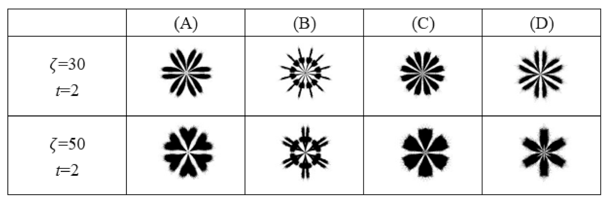
The time delay coefficient t is set as 2, which has a better identification result in the traditional vehicle. Two weighting coefficients ζ = 30 and ζ = 50 are used in this electric motor SDP application. Figure 15 shows the SDP figures for four test motors with time delay coefficient is 2 and various weights are summarized. The specifications for four test motors are summarized in Table 2. The motor noise recognition good show accuracy rate. When t = 2 and ζ = 30, it can reach 100% accuracy in 100–1500 iterative layers, and t = 2 and ζ = 50, the accuracy is 100% when the number of layers is above 300 iterative layers in the electric vehicle experimental work. Further work will focus on extending to the electric motor fault diagnosis.

Figure 15.
SDP figures of four test motors with time delay coefficient is 2 with various weighting coefficient for four different types.
Table 2.
Electrical vehicle specifications in the experiment.
5. Conclusions
This research recognizes different types of vehicle noise using the sound symmetry point pattern, and convolutional neural network technology to classify the symmetry point pattern, achieving the purpose of different vehicle classification. In the experimental work, the traditional internal combustion engine and electric vehicle were studied. During this research the time delay coefficient and weighting coefficient in the symmetry point diagram and the number of iteration layers in the neuron-like neurons were used as parameters to explore the influence of each variable on the recognition rate. The experimental results indicated that the SDP can successfully demonstrate vehicle noise characteristics and classification. The parameters of SDP are also studied in experimental case. The SDP coefficient ratio suitable for vehicle noise can be effectively identified. This method can effectively identify the sound of different vehicle motor conditions. This experiment extends the technology to apply in electric motors. It was found that the SDP diagram can also effectively display the noise characteristics of electric motors. The SDP diagram can be used to identify the four different electrical vehicle motors.
Author Contributions
Conceptualization, J.-D.W.; formal analysis, W.-J.L.; funding acquisition, J.-D.W.; methodology, J.-D.W. and K.-C.Y.; software, W.-J.L.; supervision, J.-D.W. and K.-C.Y.; writing—original draft, W.-J.L.; writing—review and editing, J.-D.W. and W.-J.L. All authors have read and agreed to the published version of the manuscript.
Funding
The research was funded by the Ministry of Science and Technology of Taiwan, Republic of China, grant number MOST 109-2221-E-018-013.
Conflicts of Interest
The authors declare no conflict of interest.
References
- Pickover, C.A. On the use of symmetrized dot patterns for the visual characterization of speech waveforms and other sampled data. J. Acoust. Soc. Am. 1986, 80, 955–960. [Google Scholar] [CrossRef] [PubMed]
- Derosier, B.; Normand, M.; Peleg, M. Effect of lag on the symmetrized dot pattern (SDP) displays of the mechanical signatures of crunchy cereal foods. J. Sci. Food Agric. 1997, 75, 173–178. [Google Scholar] [CrossRef]
- Shibata, K.; Takahashi, A.; Shirai, T. Fault diagnosis of rotating machinery through visualization of sound signals. J. Mech. Syst. Signal Process. 2000, 14, 229–241. [Google Scholar] [CrossRef]
- Dudkowska, A.; Makowiec, D. Sleep and wake phase of heart beat dynamics by artificial non symmetrized patterns. Phys. A Stat. Mech. Appl. 2004, 336, 174–180. [Google Scholar] [CrossRef]
- Wu, J.D.; Chuang, C.Q. Fault diagnosis of internal combustion engines using visual dot patterns of acoustic and vibration signals. NDT E Int. 2005, 38, 605–614. [Google Scholar] [CrossRef]
- Yang, C.; Feng, T. Abnormal noise diagnosis of internal combustion engine using wavelet spatial correlation filter and symmetrized dot pattern. Appl. Mech. Mater. 2011, 141, 168–173. [Google Scholar] [CrossRef]
- Tomasz, F.; Štefan, L. Assessment of the vibro activity level of SI engines in stationary and non-stationary operating conditions. J. Vibro Eng. 2014, 16, 1349–1359. [Google Scholar] [CrossRef]
- Wang, J.C. Vehicle Type Identification Using Visual Dot Pattern Technique of Noise Signal. Master’s Thesis, National Changhua University of Education, Changhua, Taiwan, 2015. [Google Scholar]
- Hubel, D.H.; Wiesel, T.N. Receptive fields, binocular interaction and functional architecture in the cat’s visual cortex. J. Physiol. 1962, 160, 106–154. [Google Scholar] [CrossRef]
- Fukushima, K. Neocognitron: A self-organizing neural network model for a mechanism of pattern recognition unaffected by shift in position. Biol. Cybern. 1980, 36, 193–202. [Google Scholar] [CrossRef]
- Krizhevsky, A.; Sutskever, I.; Hinton, G.E. Imagenet classification with deep convolutional neural networks. Adv. Neural Inf. Process. Syst. 2012, 25, 1097–1105. [Google Scholar] [CrossRef]
- Vedaldi, A.; Lenc, K. Matconvnet: Convolutional neural networks for MATLAB. In Proceedings of the 23rd ACM International Conference on Multimedia, Brisbane, Australia, 26–30 October 2015; pp. 689–692. [Google Scholar] [CrossRef]
- Konovalenko, I.; Maruschak, P.; Prentkovskis, O.; Junevičius, R. Investigation of the rupture surface of the titanium alloy using convolutional neural networks. J. Mater. 2018, 11, 2467. [Google Scholar] [CrossRef] [PubMed] [Green Version]
- Abiyev, R.H.; Ma’aitah, M. Deep convolutional neural networks for chest diseases detection. J. Healthc. Eng. 2018, 1, 11. [Google Scholar] [CrossRef] [PubMed] [Green Version]
- Kalfas, I.; Vinken, K.; Vogels, R. Representations of regular and irregular shapes by deep convolutional neural networks, monkey infero temporal neurons and human judgments. J. PLoS Comput. Biol. 2018, 14, 10. [Google Scholar] [CrossRef]
- Jain, K.; Choudhury, T.; Kashyap, N. Smart vehicle identification system using OCR. In Proceedings of the 2017 3rd International Conference on Computational Intelligence and Communication Technology (CICT), Ghaziabad, India, 9–10 February 2017; pp. 3–6. [Google Scholar] [CrossRef]
- Zhang, X.; Jiang, L. Vehicle types recognition based on neural network. Int. Conf. Comput. Intell. Nat. Comput. 2009, 1, 3–6. [Google Scholar] [CrossRef]
- Zeng, R.; Zhang, L.; Xiao, Y.; Mei, J.; Zhou, B.; Zhao, H.; Jia, J. An approach on fault detection in diesel engine by using symmetrical polar coordinates and image recognition. Adv. Mech. Eng. 2014, 6, 273929. [Google Scholar] [CrossRef]
- González, J.; Oro, F.M.J.; Méndez, D.; Argüelles, K.M.; Velarde-Suárez, S.; Rodríguez, D. Symmetrized dot pattern analysis for the unsteady vibration state in a sirocco fan unit. Appl. Acoust. 2019, 152, 1–12. [Google Scholar] [CrossRef]
- Nilwong, S.; Hossain, D.; Kaneko, S.-I.; Capi, G. Deep Learning-Based Landmark Detection for Mobile Robot Outdoor Localization. Machines 2019, 7, 25. [Google Scholar] [CrossRef] [Green Version]
- Li, Y.; Yang, F.; Zha, W.; Yan, L. Combined Optimization Prediction Model of Regional Wind Power Based on Convolution Neural Network and Similar Days. Machines 2020, 8, 80. [Google Scholar] [CrossRef]
- Pham, M.-T.; Kim, J.-M.; Kim, C.-H. 2D CNN-Based Multi-Output Diagnosis for Compound Bearing Faults under Variable Rotational Speeds. Machines 2021, 9, 199. [Google Scholar] [CrossRef]
- Colantonio, L.; Equeter, L.; Dehombreux, P.; Ducobu, F. A Systematic Literature Review of Cutting Tool Wear Monitoring in Turning by Using Artificial Intelligence Techniques. Machines 2021, 9, 351. [Google Scholar] [CrossRef]
- Fentaye, A.D.; Zaccaria, V.; Kyprianidis, K. Aircraft Engine Performance Monitoring and Diagnostics Based on Deep Convolutional Neural Networks. Machines 2021, 9, 337. [Google Scholar] [CrossRef]
- Gong, L.; Fan, S. A CNN-Based Method for Counting Grains within a Panicle. Machines 2022, 10, 30. [Google Scholar] [CrossRef]
- Georgescu, M.; Ionescu, R.T. Recognizing facial expressions of occluded faces using convolutional neural networks. Int. Conf. Neural Inf. Process. 2019, 1142, 645–653. [Google Scholar] [CrossRef] [Green Version]
- Knauer, U.; Rekowski, C.S.; Stecklina, M.; Krokotsch, T.; Minh, T.P.; Hauffe, V.; Kilias, D.; Ehrhardt, I.; Sagischewski, H.; Chmara, S.; et al. Tree species classification based on hybrid ensembles of a convolutional neural network (CNN) and random forest classifiers. Remote Sens. 2019, 11, 2788. [Google Scholar] [CrossRef] [Green Version]


Publisher’s Note: MDPI stays neutral with regard to jurisdictional claims in published maps and institutional affiliations. |
© 2022 by the authors. Licensee MDPI, Basel, Switzerland. This article is an open access article distributed under the terms and conditions of the Creative Commons Attribution (CC BY) license (https://creativecommons.org/licenses/by/4.0/).