Model Reference Adaptive Control-Based Autonomous Berthing of an Unmanned Surface Vehicle under Environmental Disturbance

Abstract

Surface-vehicle berthing is a complex and challenging task. It involves complicated ship dynamics owing to a large drift angle and the time-varying environmental disturbances induced by wind, wave, and current. Therefore, berthing requires state processing at each step and a controller that can respond to the non-linear behavior of the unmanned surface vehicle (USV). Herein, a systematic approach for the autonomous berthing of a USV is proposed. A state-machine approach is proposed to solve state transitions in the berthing step. A model reference adaptive controller was adopted to cope with the uncertainty of USV dynamics during berthing. Herein, the theoretical background and design of the adaptive controller are described. Simulation for the validation of the proposed method was conducted using the robot operating system Gazebo-based simulator. Finally, the respective performances of the proposed method and conventional controller were compared. Using the proposed berthing approach, an accurate and stable docking of small USVs became achievable.

1. Introduction

Small boats have been receiving considerable attention worldwide for various activities, such as leisure and travel. According to Global Market Insights, a market-research company, the estimated size of the small-boat market was approximately 35 billion US dollars in 2020, an increase of approximately 10 billion US dollars over the approximate market size of 24 billion US dollars in 2017. By 2027, the market size is predicted to be 60 billion US dollars, which is double the current market size.

When operating a ship, along with general navigation, an important process is unberthing/berthing. Berthing is the operation that allows the ship to be anchored close to the quay wall. However, the sea environment may cause the ship to slip. Therefore, predicting the behavior of the ship is difficult, and the ship may collide with the quay wall. In addition, because the ship operates at a low speed during berthing, its steering performance may deteriorate. Moreover, environmental disturbances, such as currents, winds, and waves, significantly affect operation. Therefore, an accurate control of the ship is required more during berthing than during navigation.

The case of an accident in which a collision occurs between a ship and quay wall is depicted in Figure 1. Using merely a linear PID controller in such an environment, a robust control of the ship is difficult. Research on the automatic berthing of ships is actively being conducted.

The study by [1] marked the beginning of research on automatic berthing. As described above, the low speed of the ship reduces the control force, which easily affects the behavior of the ship during environmental disturbances. Owing to the non-linear behavior of those ships, ref. [1] attempted to establish a berthing method that was not standardized as an expert system. Although the standardization of the berthing method was suggested using the expert system, the method was relatively simple. The target vessel was selected for its holonomic behavior in the final berthing stage. Therefore, the applicable vessels were limited. The authors in [2] studied and proposed a similar berthing method using a neural network that does not require ship dynamics. This was also due to the non-linear behavior of the vessel when berthing. However, because the method considered only the relatively simple berthing process of a large ship, performing all precise berthing processes was insufficient. In the study by [3], a learning method was adopted using a head-up coordinate system to overcome the limitations of the Artificial Neural Network (ANN) berthing method applicable only at learned ports. Authors in [4] also attempted to overcome the limitations of the ANN berthing method by learning using a distance-measurement system. Although the above three studies proposed berthing methods using ANN, they omitted the final berthing step and were limited to navigating the vessel near the port.

Furthermore, the authors in [5] suggested a method for efficient path planning for ships. Research [6] proposed a method that considers ocean current in the existing path-planning method. Both studies focused on path planning instead of a comprehensive berthing process. In the studies by [7,8,9], ships equipped with bow thrusters and capable of pure sway motion were considered. In addition to the previous studies, research has been conducted considering the entire berthing process, including the final berthing process, which is difficult to control. However, the methods proposed in these studies have limitations, because they can only be applied to ships capable of pure sway motion. To summarize, most studies on large ships and ships with underactuated propulsion systems in the final stage of berthing are insufficient.

Now, The study of berthing for a small boat is as follows. In [10], the authors used ANN and validated the proposed method using the Monte Carlo simulation. However, the study was conducted considering that the boat was approaching the port after a straight voyage, and only the starting point varied. Authors in [11] proposed a method of changing the state of the berthing method. It was based on the distance of the boat from the berthing point and a method of navigating the vessel near a port. In [12], the authors attempted to increase the accuracy of berthing from near the port to the final berthing point by using internal model control (IMC). However, the study had a limitation in that it considered only the ships capable of pure sway motion. In the study of [13], a similar berthing method was presented using IMC. Unlike [12], the berthing method was presented from the approach state. However, similar to the above method, this method can also be applied only to the ships capable of pure sway motion. As such, studies on the automatic berthing of small boats are rare, and most of the studies are aimed at ships capable of pure sway motion. However, in the case of small boats manufactured for leisure or research purposes, such studies are difficult to implement, because most of the ships are not equipped with bow thrusters.

In this study, an automatic berthing method for a small underactuated ship in an environment with disturbances is proposed. In the proposed method, a state machine was used to establish the berthing of the vessel in a step-by-step manner, so that it responded to failure conditions. A model reference adaptive control strategy was used to normalize the operation of the ship by applying the appropriate control in response to the unpredictable and uncertain ship behavior. In addition, verification through simulation was performed in the Gazebo environment of the robot operating system (ROS), which implements an environment similar to the actual sea environment.

The contribution of this study can be roughly divided into two categories. First, adaptive control, which has been applied to various problems, was applied to the automatic berthing problem of small boats. As mentioned above, unlike large vessels, few studies have been reported on the automatic berthing of small boats. Studies on techniques for sophisticated control are also scarce. Therefore, in this study, an automatic berthing formulation of a small boat is proposed. The formulation defines the scenario of the most representative problem situation and provides the relevant results. Based on those data, the method is expected to serve as a reference for similar studies in the future. Second, the automatic berthing method proposed in this study was simulated in the environment of ROS Gazebo, which has the advantage of reflecting precise models for environmental loads. Moreover, in this operating system, various sensors can be modeled, and it is possible to consider the collision between objects to be reflected in the berthing problem. Therefore, ROS Gazebo enables integrated control simulation and is currently widely used in the robotics field. In the present study, for the first time, Gazebo was applied to the berthing problem of unmanned surface vehicles (USVs).

This paper is organized as follows. Section 2 establishes the berthing path planning suitable for the berthing location, based on the state machine, and presents the proposed berthing method. Section 3 describes the vector-field guidance law to follow the planned path and the design of the MRAC controller used in this study. Section 4 presents the simulation and theoretical verification in the ROS Gazebo environment. Finally, Section 5 presents the conclusions and considerations of this study.

2. Berthing Path Planning

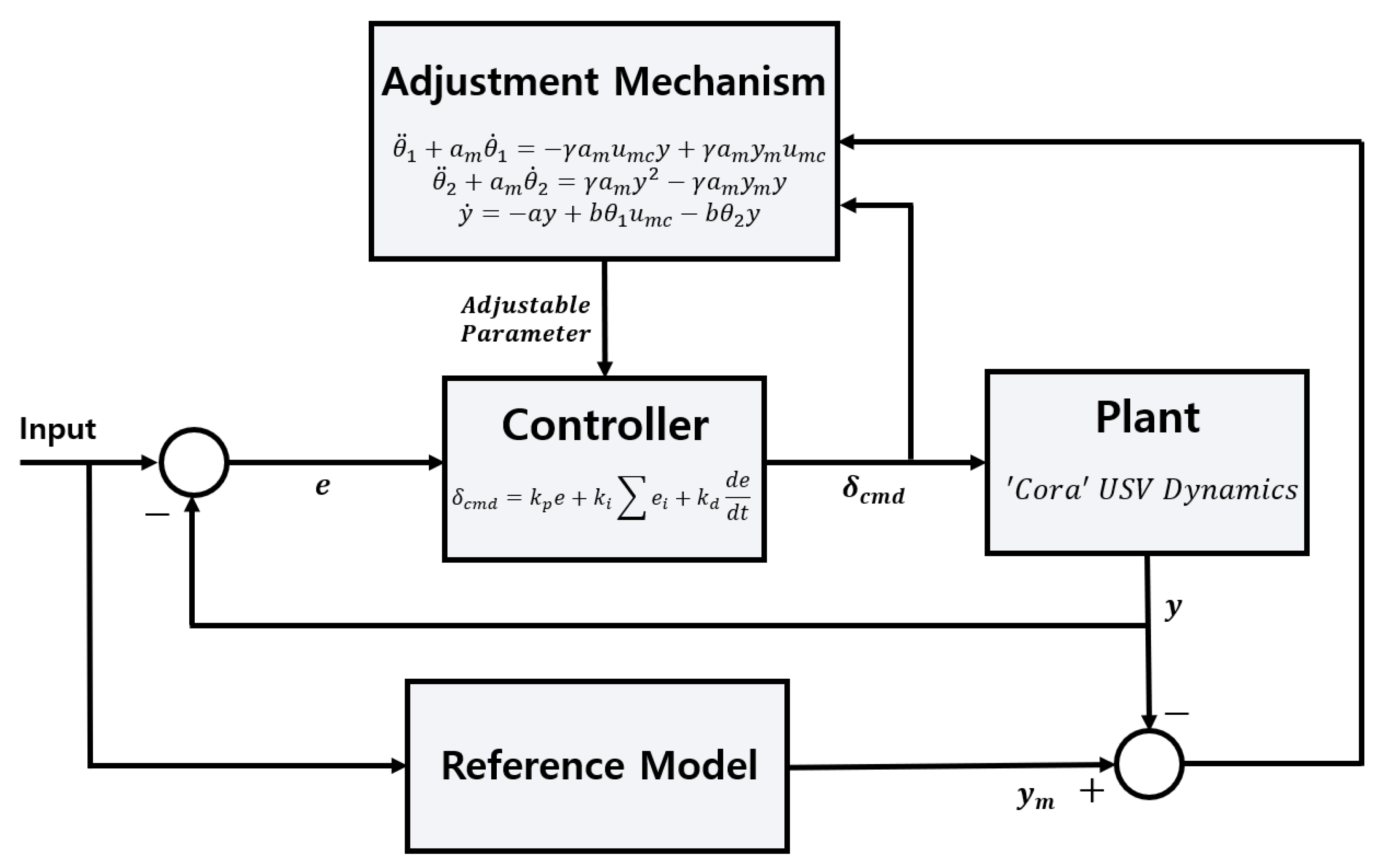
The target vessel in this study was a small boat, such as a USV. Small boats often find themselves in environments such as a marina. A general marina can be divided into two docking types. In the first type, a USV enters the docking position in the direction of the USV bow. Therefore, when it is adjacent to the docking position, as shown in Figure 2 (left), it moves to the target docking point following a curve. In this paper, this docking type is defined as the parallel type. In some cases, it is impossible to dock forward owing to the marina environments and facilities. In such a case, as shown in Figure 2 (right), a USV moves close to the docking position, follows a curve, and gradually moves away from the docking position—thereby making the angle at which the USV can be docked backward. Finally, the USV slowly retreats and docks at the docking position. This docking type is defined as the finger type. In both types, berthing is performed on the basis of the state machine.

Figure 3 shows the state machines of the parallel and finger types, where $d_A$ is the distance between the USV and the path tracking starting point, $d_F$ is the distance between the USV and the starting point, $d_C$ is the distance between the USV and the destination, $d_0$ is the distance between the USV and the docking station, and t is time to arrive at the destination. The parallel-type docking starts from the approach state. The approach state is the same state as ➀ in Figure 2 (left). In this state, the USV approaches the point where it has to start turning for berthing. In this state, if the distance between the USV and the destination is smaller than the length of the USV, it proceeds to the next state—the alignment tracking state. It is the same as ➁ in Figure 2 (left). In this state, the USV turns to the docking target point and tracks the curve. Similarly, to move from the current state to the next, if the distance to the docking target point is smaller than the length of the USV, the docking process proceeds to the next state, i.e., the docking state. The docking state corresponds to ➂ in Figure 2 (left). In this state, the turning speed of the USV is reduced, so that it can be finally docked. When transitioning from the previous state, the docking process reverses the current direction to reduce the USV’s speed and provides the Rudder command to approach the rock wall at a low speed. If the distance error from the berthing arrival point does not exceed 10% of the USV’s length and lasts for more than 3 s, docking is judged to be completed.

The finger-type approach is also the same state as ➀ in Figure 2 (right). In this state, the USV approaches the berthing point by tracking a straight line to the turning point for berthing. Similarly, if the distance from the turning point to the USV is smaller than the USV length, the docking process transitions to the next state. The forward-alignment tracking state is the same state as ➁ in Figure 2 (right). In this state, the USV turns to form a heading angle to approach the docking target point backward. The curve approaches the target point by path tracking. When the distance from the target point to the USV becomes smaller than the length of the USV, the docking process transitions to the next state. That is the back-alignment tracking state, which is the same as ➂ in Figure 2 (right). Based on the heading angle set in the previous forward-alignment tracking state, straight-path tracking is performed backward to the final berthing target point. If the distance from the target point to the USV becomes smaller than the length of the USV, the docking process transitions to the next state, i.e., the docking state. This state corresponds to ➃ in Figure 2 (right). When crossing over from the previous state, the direction of travel of the USV is reversed to reduce its speed. This state provides the Rudder command value, so that the USV can approach the docking target point at a slow speed. When the distance error from the final destination to the USV does not exceed 10% of the USV’s length for more than 3 s, berthing is judged to be completed.

3. Control System

For a USV to accurately berth, it is necessary to accurately follow the planned path. Therefore, in this study, path tracking was performed using vector-field path following—proposed by [14]. Figure 4 illustrates this the vector field. In linear path tracking, the vector field corresponds to the angle from Waypoint1 to Waypoint2, $waypoint1=[w_{1_x},w_{1_y}]$ and $waypoint2=[w_{2_x},w_{2_y}]$, ${\chi }^f$ can be expressed as

$${\chi }^f=atan2(w_{2_{y-w_{1_y}}},w_{2_{x-w_{1_x}}}).$$

(1)

${\chi }^a$ is the entry heading angle, as shown in Figure 5. $ϵ$ is the cross-track error, the vertical distance between the path and the USV. $\tau$ represents the boundary distance to the transition region, which can be confirmed in Figure 5. The USV approaches the path at an angle of ${\chi }^a$, irrespective of its location. If the cross-track error is less than $\tau$, it follows the target angle with a value different than the calculated value. Therefore, linear path tracking of the vector field can be explained by the following Equation (2):

$${\chi }^d={\chi }^f-\left({\chi }^a\right){\left(\frac{ϵ}{\tau }\right)}^k$$

(2)

At this time, k is the transition gain and it is greater than 1.

The following describes the path tracking of the USV for the circular path. In the case of linear path, the target heading angle is changed based on the value of $\tau$; it plays this role in the circular path. The target heading angle is changed based on the value of $2R$ in the circular path. Here, $2R$ denotes the radius of the circle to be tracked. $\beta$ is the angle from the center of the circle to the USV, as shown in Figure 6. d is the straight-line distance from the center of the circle to the USV. Therefore, the desired heading angle in the circular path is expressed in Equations (3) and (4) as follows (when clockwise):

$$ifd>2R$$

$${\chi }^d=\beta +\frac{5\pi }{6}$$

(3)

$$else$$

$${\chi }^d=\beta +\frac{\pi }{2}+\left(\frac{\pi }{3}\right){\left(\frac{d-R}{R}\right)}^k$$

(4)

In the cases of straight and curved path tracking in this study, the vector-field path following was used.

The heading angle of the USV was controlled through a PID controller, which is the most used controller for path tracking during berthing. In this study, the adaptive gain was tuned through adaptive control—considering wind disturbance in the environment of the USV. An adaptive control system adjusts the control over time, according to the changing conditions and the knowledge it acquires. In particular, adaptive control improves the controller by actively responding to the changes in the system instead of remaining static or ignoring the minor deviations. This method is necessary for dynamic systems in unstable environments—such as aircraft and medical robots. However, when a USV is berthing, the wind makes its operation unstable. Therefore, in this study, the design proposal applied adaptive control to USV berthing.

In this study, among the adaptive control schemes, the model reference adaptive control (MRAC) scheme was used. In MRAC, the required system performance is defined via a reference model. It has the desired response to a command value and the control system follows the behavior of this reference model.

In this study, before designing the controller, the USV’s system identification process for wind environments was performed from various angles. The system identification was conducted in the Gazebo environment of ROS. The detailed description of Gazebo is presented in Section 4. During system identification, the transfer-function model of the USV system was derived by analyzing the USV’s response to the direction in which it faced the wind. The wind was set to be flowing at Beaufort 6. The angle between the USV and the wind is defined as the encounter angle. The encounter-angle range of 0°–360° was divided into 12 sections at 30° intervals. The reference model was derived from the MRAC through the following system identification task.

When designing a controller, the typical adaptation mechanisms of MRAC are the MIT Rule based on gradient method, and the Lyapunov Rule based on the Lyapunov Stability Theory. In this study, the MIT Rule was employed as the adaptation mechanism [15]. The rule is an early approach to MRAC, developed by the Draper Laboratory of the Massachusetts Institute of Technology (MIT) in the United States. Assuming that the controller is in a closed-loop system and has adaptive parameters, its response can be expressed as Equation (5); and its reference response can be expressed as Equation (6)

$$y=G_{L\left(s\right)u_{m_c}}$$

(5)

$$y_m=G_{m\left(s\right)u_{m_c\prime }}$$

(6)

where $G_L\left(s\right)$ is the transfer function of the system to be controlled, $G_m\left(s\right)$ is the transfer function of the desired system, and $u_{m_c}$ is the control input. The difference between the responses of the actual closed-loop system and the reference closed-loop system is called as the adaptation error, expressed as $e=y_m-y$. In this study, the loss function J was minimized by adjusting the adaptive parameter $\theta$, expressed in Equation (7) as follows:

$$J=\frac{1}{2}{e}^2$$

(7)

To minimize the loss function J, it is reasonable to adjust the adaptive parameter so that the slope of the former $\partial J/\partial \theta$ with respect to the latter $\theta$ is negative. This can be expressed as:

$$\frac{\partial \theta }{dt}=-\gamma \frac{\partial J}{\partial \theta }=-\gamma e\frac{\partial e}{\partial \theta },$$

(8)

where $\gamma$ is the adaptive gain. Equation (8) can be re-expressed as Equation (9).

$$\frac{\partial \theta }{dt}=-\gamma \frac{\partial e}{\partial \theta }e=-\frac{1}{2}\gamma \frac{\partial {\left[G_{m\left(s\right)-G_L\left(s\right)}\right]}^2}{\partial \theta }{\left(u_{m_c}\right)}^2$$

(9)

It can be observed in Equation (9) that the rate of change of the adaptive parameter is proportional to the square of the control input $u_{m_c}$—therefore, the adaptive parameter is considerably sensitive to the control input. Since the rate of change in MIT Rule is proportional to the square of the control input, it is necessary to normalize the adaptation law—expressed in Equation (10).

$$\frac{\partial \theta }{dt}=\gamma \frac{\phi }{\mu +{\phi }^T\phi }e$$

(10)

$\phi =-\partial e/\partial \theta$ is called as the sensitivity derivative. It is the parameter that prevents the division of $\mu >0$ by zero. The structure of the MRAC controller used in this study is shown in Figure 7. In Equation (5), the control input is the target heading angle and the output is the yaw rate of the USV. In Equation (6), the control input is the target heading angle and the output is the yaw rate of the reference model. According to the study of [16], the reference model can be expressed by Equation (11); the input of the system can be expressed by Equation (12).

$$\frac{d{y}_m}{dt}=-a_{m{y}_m}+b_{m{u}_{m_c}}$$

(11)

$$u\left(t\right)={\theta }_1\left(t\right)u_{m_c(t})-{\theta }_2\left(t\right)y\left(t\right)$$

(12)

Here, $y_m$ and $u_{m_c}$ are the output and input values of the reference model, respectively, and $a_m$ and $b_m$ are the parameter values of the reference model. ${\theta }_1$ and ${\theta }_2$ are the adaptive parameters. Equation (8) can be expressed in terms of ${\theta }_1$ and ${\theta }_2$ as Equation (13) as follows:

$$\frac{\partial {\theta }_1}{dt}=-\alpha \frac{\partial J}{\partial {\theta }_1}=-\alpha e\frac{\partial e}{\partial {\theta }_1}$$

$$\frac{\partial {\theta }_2}{dt}=-\alpha \frac{\partial J}{\partial {\theta }_2}=-\alpha e\frac{\partial e}{\partial {\theta }_2}$$

(13)

According to the study of [16], ${\theta }_1$ and ${\theta }_2$ are updated based on Equation (14).

$$\ddot{{\theta }_1}+a_m\dot{{\theta }_1}=-\gamma a_m{u}_{m_c}y+\gamma a_m{y}_{m{u}_{m_c}}$$

$$\ddot{{\theta }_2}+a_m\dot{{\theta }_2}=\gamma a_m{y}^2-\gamma a_m{y}_{m}y$$

$$\dot{y}=-ay+b{\theta }_1{u}_{m_c}-b{\theta }_{2}y$$

(14)

Therefore, if the adaptive controller is designed using the above equation, the system response varies based on the adaptive gain $\gamma$.

Figure 8 shows the system response according to the input value of each system according to $\gamma$ through a 3-2-1-1 test. $r_d$ represents the desired yaw rate and is the standard value of the 3-2-1-1 test with the size of 70% of the maximum yaw rate. $r_{{\gamma }_{0.5}},r_{{\gamma }_2},r_{{\gamma }_{3.5}}$ corresponds to the yaw rate when $\gamma$ values are 0.5, 2, and 3.5, respectively. If $\gamma$ is small, the system converges with a relatively low overshoot, but the adaptation is slow. If $\gamma$ is large, there is a large overshoot in the state, but the adaptation is considerably fast. The proof of the stability of the MRAC based on the MIT Rule can be found in [17].

4. Simulation

4.1. Assumption

The problem was simplified to achieve the purpose of the study. In this study, only the horizontal plane motion of the USV is described because the USV’s yaw-rate tracking control is performed. The motion variables of the USV based on the body-fixed coordinate system are shown in Figure 9. The simplification of the USV applied to the simulation is as follows: First, the USV’s motion neglects roll, pitch, and heave directions. Second, the USV has neutral buoyancy, and the origin of the body-fixed coordinate system is its center of mass. Third, the USV has three planes of symmetry. The above assumptions, suitable for the simulation of the USV in this study, are based on [18].

4.2. Simulation Environment

Robot simulation is an essential tool for robotics engineers. Gazebo enables robot simulation in the ROS environment. RoboNation and the U.S. Office of Naval Research (ONR) are collaborating with the U.S. Naval Postgraduate School (NPS) and Open Robotics (OR) to provide Virtual RoboX (VRX). It can simulate USVs in the Gazebo environment. VRX is an open-source simulation environment designed to help students test solutions for autonomous USVs for free. Similarly, NPS and Robonation are developing the Virtual Ocean Robotics Challenge (VORC). It is based on VRX and simulates the Ocean Robotics Challenge as a virtual environment. In this study, the simulation was performed in VORC, and the environment model of VRX, on which VORC is dependent, was used as the modeling environment. The target USV of the present study is the virtual USV ‘Cora’ on VORC. The simulation environment is shown in

Table 1. Main specifications of the USV simulation environment.

Parameter		Information
	Length [m]	12.2
USV Spec	Breadth [m]	3.3
	Hullradius [m]	2.2
Thruster	Type	Azimuth type (2ea)
	Max Angle [degree]	±35
Hull Type	-	Mono Hull
Velocity [knot]	-	4∼5
	Mean Vel [m/s]	10
Wind	Var Gain	2
	Var time [s]	1

. The structure of the thruster described in Table 1 is shown in Figure 9.

$$\begin{array}{c}\hfill M_{R_B\dot{\nu }}+C_{P{R}_B\left(\nu \right)\nu }+M_A\dot{{\nu }_r}+C_A\left({\nu }_r\right){\nu }_r+D\left({\nu }_r\right){\nu }_r+g\left(\eta \right)={\tau }_{propulsion}+{\tau }_{w_{i_{n_d}}}+{\tau }_{w_{a_{v_e}}}\end{array}$$

(15)

where

$$\begin{array}{c}\hfill \begin{array}{c}\hfill \eta ={\left[x,y,z,\pi ,\theta ,\psi \right]}^T\\ \hfill \nu ={\left[u,v,w,p,q,r\right]}^T\end{array}\end{array}$$

(16)

The USV’s maneuvering model is expressed by Equation (15). For the USV dynamics model, the reader is advised to refer to [19]. Here, $M_{R_B}$ is the added mass coefficient of the acceleration term of the rigid body and $C_{R_B}$ is the damping coefficient of the velocity term of the rigid body. $M_A$ is the added mass coefficient of the acceleration term due to the fluid force. The simplified added mass matrix is:

$$M_A=-\left[\begin{array}{cccccc}{X}_{\dot{u}}& 0& 0& 0& 0& 0\\ 0& Y_{\dot{v}}& 0& 0& 0& Y_{\dot{r}}\\ 0& 0& 0& 0& 0& 0\\ 0& 0& 0& 0& 0& 0\\ 0& 0& 0& 0& 0& 0\\ 0& N_{\dot{v}}& 0& 0& 0& N_{\dot{r}}\end{array}\right]$$

(17)

$C_A$ is the damping coefficient of the velocity term due to the fluid force.

$$C_A\left({\nu }_r\right)=\left[\begin{array}{cccccc}0& 0& 0& 0& 0& Y_{\dot{v}}{v}_r+Y_{\dot{r}}r\\ 0& 0& 0& 0& 0& -X_{\dot{u}}{u}_r\\ 0& 0& 0& 0& 0& 0\\ 0& 0& 0& 0& 0& 0\\ 0& 0& 0& 0& 0& 0\\ 0& 0& 0& -Y_{\dot{v}}{v}_r-Y_{\dot{r}}r& X_{\dot{u}}{u}_r& 0\end{array}\right]$$

(18)

$D\left({\nu }_r\right)$ is the hydrodynamic damping coefficient, including forces due to radiation-induced potential damping, skin friction, wave drift damping, vortex shedding, and lifting forces. Therefore, the hydrodynamic damping matrix can be expressed as:

$$\begin{array}{c}\hfill D\left({\nu }_r\right)=D_l+D_l\left({\nu }_r\right)\end{array}$$

(19)

$$D_l=-\left[\begin{array}{cccccc}{X}_u& 0& 0& 0& 0& 0\\ 0& Y_v& 0& 0& 0& Y_r\\ 0& 0& Z_w& 0& 0& 0\\ 0& 0& 0& K_p& 0& 0\\ 0& 0& 0& 0& M_q& 0\\ 0& N_v& 0& 0& 0& N_r\end{array}\right]$$

(20)

$$D_l\left({\nu }_r\right)=-\left[\begin{array}{cccccc}{X}_{u\left|u\right|}\left|u_r\right|& 0& 0& 0& 0& 0\\ 0& Y_{v\left|v\right|}|v_r|+Y_{\left|r\right|v}\left|r\right|& 0& 0& 0& Y_{\left|v\right|r}|v_r|+Y_{\left|r\right|r}\left|r\right|\\ 0& 0& 0& 0& 0& 0\\ 0& 0& 0& 0& 0& 0\\ 0& 0& 0& 0& 0& 0\\ 0& N_{\left|v\right|v}|v_r|+N_{\left|r\right|v}\left|r\right|& 0& 0& 0& N_{\left|v\right|r|}|v_r|+N_{r\left|r\right|}\left|r\right|\end{array}\right]$$

(21)

${\tau }_{propulsion}$ is the external force caused by the propulsion system, which was not addressed in detail in this study. The wind and wave models that affect the USV of VRX were implemented as independent model plug-ins of Gazebo. ${\tau }_{w_{i_{n_d}}}$ represents the external force applied to the USV by the wind. ${\tau }_{w_{a_{v_e}}}$ represents the external force applied to the USV by the waves. ${\nu }_c$ represents the non-rotating current, and ${\nu }_r$ represents the velocity vector relative to ${\nu }_c$. Therefore, $\nu ={\nu }_r+{\nu }_c$. Wave model on VRX Gazebo [20,21] was formulated using Gerstner wave model as:

$$X_w=X_0-\sum _{i=1}^N{q}_i{A}_{i}sin(k_i·X_0-w_{i}t+{\varphi }_i)$$

(22)

$$z=X_0-\sum _{i=1}^{N}i{A}_{i}cos(k_i·X_0-w_{i}t+{\varphi }_i)$$

(23)

The wave height z is generated at the initial position $X_0=x_0,y_0$ and $X_w=x,y$. Further, $q_i$ represents steepness and $A_i$ represents amplitude. $k_i$ denotes wave vector, $w_i$ denotes angular frequency, and ${\varphi }_i$ denotes phase. Wave vector is horizontal to the propagation direction of the wave, and the scale is the same as wave number $k=2\pi /\mathsf{\Lambda }$; where $\mathsf{\Lambda }$ is the length of the wave. The wave number and angular frequency are related to deep-water dispersion by Equation (24). The wave height z of the transient state occurring at the beginning of the simulation is expressed as Equation (25).

$$w^2=gk$$

(24)

$$z=(1-e^{-t/\tau })\sum _{i=1}^N{A}_{i}cos(k_i·X_0-w_{i}t+{\varphi }_i)$$

(25)

The Wavefield model uses two of the Pierson–Moskowitz wave spectra and the constant wavelength-to-amplitude ratio. Wind force (x and y) and moment (yaw) of the model plugin are based on the model proposed by Fossen [22]. Let the velocity vector of the wind be $V_R$. The three-degree-of-freedom force and moment of motion in the horizontal plane can be expressed by Equations (26)–(28).

$$X_{wind}=\left(C_X\right)V_{R_x}\left|V_{R_x}\right|$$

(26)

$$Y_{wind}=\left(C_Y\right)V_{R_y}\left|V_{R_y}\right|$$

(27)

$$N_{wind}=-2.0\left(C_N\right)V_{R_x}{V}_{R_y}$$

(28)

In these equations, $C_X$, $C_Y$, and $C_N$, representing the coefficients of wind in each direction, are calculated by the formula proposed by Sarda [23]. The modeling of wind irregularities was performed on the basis of the study of VRX Gazebo [19]. If the constant average wind speed is $\overline{v}$, and the temporarily variable wind speed is $v_g\left(t\right)$, the total wind speed $V_w\left(t\right)$ can be expressed by Equation (29).

$$V_w\left(t\right)=\overline{v}+v_g\left(t\right)$$

(29)

The wind speed can be specified by various user-specified variables, such as constant wind direction ${\beta }_w$, constant wind speed $\overline{v}$, standard deviation ${\sigma }_g$, and time constant ${\tau }_g$. The variable component of wind speed is modeled as a first-order linear approximation of the Harris spectrum [24] with a time constant ${\tau }_g$. The spectrum is expressed as a transfer function of the Equation (30), where $K_w$ is the amplitude of the response. The variable wind speed at discrete time $K+1$ is expressed by Equation (31).

$$h\left(s\right)=\frac{K_w}{1+{\tau }_{g}s}$$

(30)

$$v_g[k+1]=v_g\left[k\right]+(1/{\tau }_g)(-v_g\left[k\right]+K_{w}n\left[k\right])\delta t$$

(31)

$n\left[k\right]$ is a Gaussian distribution, a pseudorandom number generated with zero mean and unit variance. $\delta t$ is the simulation time step. The spectrum of the variable wind speed produced by Equation (31) is expressed as Equation (32).

$$s_g\left(w\right)=\left\{\begin{array}{cc}\frac{K_w^2}{1+{\left(w{\tau }_g\right)}^2}\hfill & \left|w\right|<w_s/2\hfill \\ 0\hfill & \left|w\right|\ge w_s/2\hfill \end{array}\right.$$

(32)

where $w_s$ is the sampling frequency and $w_s=2\pi /\delta t$. Assuming that $w_s\gg 2\pi /T$ are the standard deviation and time constant specified by the user, respectively, the parameter $K_w$ required to generate the variable-wind component can be expressed as Equation (33).

$$K_w={\sigma }_g\sqrt{\frac{2{\tau }_g}{\delta t}}$$

(33)

The user can change the wind direction, average speed, magnitude of deviation, and change time by setting the simulation environment. The values can be respectively applied to the wind model. In the present study, the wind direction in the simulation is as shown in Figure 10. The average speed is 10 m/s. The magnitude of deviation is doubled and the change time is 1 s. Figure 10 shows the initial and final docking positions of the USV.

4.3. Berthing Simulation

The simulation results represent a case study conducted in a parallel-type simulation environment. The most representative and basic control method, the PID controller, was selected for comparison. To accurately compare the performances of MRAC and PID, the gains of the PID controller had to be properly tuned. After gain tuning, the PID controller yielded a response similar to that of the MRAC in the absence of disturbance. The absolute wind direction was set to Beaufort 6 in one direction on Gazebo, and the time-series data of wind speed are shown in Figure 11. Figure 12 shows the course error and the position error of X and Y when using only the PID controller and when the MRAC controller is applied. Figure 12 and Figure 13 depict the state machine described in Section 2 and display the state in each graph. In Figure 12, ${\chi }_e$ represents the error between the desired yaw angle in each state and the course of angle of the USV when only the PID controller is used and the MRAC controller is applied. $P_e$ is the position error. $P_{ex}$ represents the X-coordinate error between the target point and the USV in each state. $P_{ey}$ represents the Y-coordinate error between the target point and the USV in each state. The contents of $P_{ex}$ and $P_{ey}$ are the same as in Equation (34).

$$P_e=P_{USV}-P_{Destination}$$

(34)

Figure 12 shows the command value of the thruster in each state. It can be observed that the speed and angle commands of the thruster change according to the state.

The operation is divided into different states and analyzed. The approach state operates from 0 s to approximately 38 s. The linear path tracking described in Section 2 is performed. The desired heading angle is determined based on Equation (2) of Section 2. Thus, the USV follows the linear path according to the desired heading angle. The course and position errors in the windy environment are smaller in the state using the MRAC than in the state using the PID controller. The speed of convergence of state to 0 is fast. Thus, the USV to which the MRAC is applied demonstrates better path-tracking accuracy, compared to that which the PID control is applied.

The alignment tracking state operates approximately from 38 to 59 s. In this state, the circular-type path tracking is performed, as presented in Section 2. The desired heading angle is determined based on Equations (3) and (4). The USV using only the PID controller with the desired heading angle follows based on the general PID control command, and the USV applying the MRAC controller follows the adaptive control command considering the environment. When the MRAC controller is applied, the error value decreases faster even in the curve case and converges to 0. Therefore, even on a circular path, a USV to which the MRAC controller is applied shows a high path-tracking accuracy.

As shown in Figure 13 in the final-docking state, the forward speed is reduced through reverse propulsion for berthing of the USV. The thruster angle is controlled to be in the direction opposite to the rock wall to get close to it. In Figure 12, it can be observed that the position error gradually decreases and converges to 0. Therefore, the USV slows down near the berthing arrival point. When the forward speed becomes approximately 0, the USV gradually approaches the rock wall.

Figure 14 shows the boxplot comparing the responses from using MRAC, and from using only the PID controller. As shown in the figure, the range of the maximum and minimum error values was reduced from approximately −17∼−13 to approximately −12∼−9. Moreover, a change in Interquartile Range (IQR) can be observed. It is defined as the value that falls within the range of the first and third quartiles. It can be seen that the range of IQR decreases from approximately −6∼2 to −4∼−1 when the MRAC controller is applied. The trajectory when the MRAC controller is applied in the Gazebo environment is shown in Figure 15. Based on the results shown in Figure 12, Figure 13, Figure 14 and Figure 15, the PID controller does not consider the windy environment and simply outputs a general command value. Therefore, it cannot make the USV follow the path quickly. Moreover, the PID controller may give an excessive input. Owing to these shortcomings, the PID controller can lead to inaccurate path tracking. However, when the MRAC controller is applied, the control is based on the transfer function derived from the encounter angle between the USV and the wind. Therefore, the MRAC outputs the command value considering the wind environment, showing higher accuracy in path tracking than PID control. Similarly, when the MRAC controller is applied, $r_d$ is the desired yaw rate created as a reference model. r is the yaw rate of the USV. At this time, $r_d$ was determined by the vector-field guidance law of the control system section. It can be seen in Figure 16 that r follows $r_d$, indicating that adaptive control was applied.

Furthermore, various scenarios were demonstrated for reliable results. The results presented in Figure 17 were simulated in an environment set with different initial positions and wind directions. In Figure 17, the trajectory for each scenario is expressed and a boxplot of the course error is presented. As can be seen in the figure, the range of IQR is reduced when the MRAC controller is used in all the three scenarios. In other words, the range of error is reduced. At this time, for the first and second scenarios from the left of Figure 17, it progressed within a wind disturbance of Beaufort 6 level. The berthing was carried out with an average velocity 4.45 knots and standard deviation 1.2 knot in the first scenario; and an average velocity 4.37 knots and standard deviation 1.32 knot in the second scenario. In the third scenario, the wind disturbance was also at Beaufort 6 level, but the range of the circular path to be followed was wide and the drift of the USV became severe. So, it berthed at an average velocity 3.7 knots and standard deviation 1.1 knot. The velocity of the USV is crucial during the berthing process and is required to be studied in depth. However, in this study, the accuracy of path tracking was evaluated assuming only the typical berthing velocity of USVs.

5. Conclusions

The automatic berthing of ships is a difficult problem in the development of autonomous ships. Most existing studies focus on limited situations, such as targeting large ships or ships capable of pure sway motion. Therefore, their findings are not applicable to a small boat developed for general leisure or a USV developed for research purposes.

Therefore, in this study, the berthing process of a small boat in the presence of environmental disturbance was defined through a state machine. The berthing accuracy was improved using the MRAC method. The complex berthing process was systematically accumulated by expressing it as a state transition using the state machine in the berthing environment of a small boat. The MRAC controller was designed via system identification and adaptive parameter tuning. Consequently, as mentioned in the simulation section, the berthing process was a systematic state transition. Moreover, when the MRAC method was applied, the range of error decreased by more than $20\%$ on average, for various initial positions and wind direction cases.

In this study, ROS Gazebo simulation was conducted, where in dynamics and external environmental forces were precisely modeled. Although the factors necessary for the berthing study are well reflected in the simulation, they are different from the actual experimental results; this is because environmental disturbances in real seas are difficult to predict/simulate, and sensor-measurement errors may occur in real environments. Therefore, generating actual experimental results will be helpful in validating the proposed method. In the future, there is a plan to verify the validity of this study through experiments in more diverse environments and various types of docks using the USV at sea.

References

1. Yamato, H.; Koyama, T.; Nakagawa, T. Automatic berthing using the expert system. IFAC Proc. Vol. 1992, 25, 173–184. [Google Scholar] [CrossRef]
2. Zhang, Y.; Hearn, G.E.; Sen, P. A multivariable neural controller for automatic ship berthing. IEEE Control Syst. Mag. 1997, 17, 31–45. [Google Scholar] [CrossRef]
3. Im, N.K.; Nguyen, V.S. Artificial neural network controller for automatic ship berthing using head-up coordinate system. Int. J. Nav. Archit. Ocean Eng. 2018, 10, 235–249. [Google Scholar] [CrossRef]
4. Nguyen, V.S.; Do, V.C.; Im, N.K. Development of automatic ship berthing system using artificial neural network and distance measurement system. Int. J. Fuzzy Log. Intell. Syst. 2018, 18, 41–49. [Google Scholar] [CrossRef] [Green Version]
5. Djouani, K.; Hamam, Y. Minimum time-energy trajectory planning for automatic ship berthing. IEEE J. Ocean. Eng. 1995, 20, 4–12. [Google Scholar] [CrossRef]
6. Liu, C.; Mao, Q.; Chu, X.; Xie, S. An improved A-star algorithm considering water current, traffic separation and berthing for vessel path planning. Appl. Sci. 2019, 9, 1057. [Google Scholar] [CrossRef] [Green Version]
7. Park, J.Y.; Kim, N. Modeling and controller design of crabbing motion for auto-berthing. J. Ocean Eng. Technol. 2013, 27, 56–64. [Google Scholar] [CrossRef]
8. Park, J.Y.; Kim, N. Design of an adaptive backstepping controller for auto-berthing a cruise ship under wind loads. Int. J. Nav. Archit. Ocean Eng. 2014, 6, 347–360. [Google Scholar] [CrossRef] [Green Version]
9. Lee, S.; Hwang, Y.; Kim, Y. Crabbing simulation of ship with twin rudder and twin skeg. In Proceedings of the Annual Spring Meeting; Society of Naval Architects of Korea: Daejeon, Korea, 2000; pp. 144–147. [Google Scholar]
10. Ahmed, Y.A.; Hasegawa, K. Automatic ship berthing using artificial neural network based on virtual window concept in wind condition. IFAC Proc. Vol. 2012, 45, 286–291. [Google Scholar] [CrossRef]
11. Xiong, Y.; Yu, J.; Tu, Y.; Pan, L.; Zhu, Q.; Mou, J. Research on data driven adaptive berthing method and technology. Ocean Eng. 2021, 222, 108620. [Google Scholar] [CrossRef]
12. Tzeng, C.; Lee, S.; Ho, Y.; Lin, W. Autopilot design for track-keeping and berthing of a small boat. In Proceedings of the 2006 IEEE International Conference on Systems, Man and Cybernetics, Taipei, Taiwan, 8–11 October 2006; Volume 1, pp. 669–674. [Google Scholar]
13. Lee, S.D.; Tzeng, C.Y.; Shu, K.Y. Design and experiment of a small boat auto-berthing control system. In Proceedings of the 2012 12th International Conference on ITS Telecommunications, Taipei, Taiwan, 5–8 November 2012; pp. 397–401. [Google Scholar]
14. Nelson, D.R.; Barber, D.B.; McLain, T.W.; Beard, R.W. Vector field path following for miniature air vehicles. IEEE Trans. Robot. 2007, 23, 519–529. [Google Scholar] [CrossRef] [Green Version]
15. Mareels, I.M.; Anderson, B.D.; Bitmead, R.R.; Bodson, M.; Sastry, S.S. Revisiting the MIT rule for adaptive control. In Adaptive Systems in Control and Signal Processing 1986; Elsevier: Amsterdam, The Netherlands, 1987; pp. 161–166. [Google Scholar]
16. Åström, K.J.; Wittenmark, B. Adaptive Control; Courier Corporation: North Chelmsford, MA, USA, 2013. [Google Scholar]
17. Mareels, I.; Ydstie, B. Global stability for an MIT rule based adaptive control. In Proceedings of the 28th IEEE Conference on Decision and Control, Tampa, FL, USA, 13–15 December 1989; pp. 1585–1590. [Google Scholar]
18. Vu, M.T.; Van, M.; Bui, D.H.P.; Do, Q.T.; Huynh, T.-T.; Lee, S.-D.; Choi, H.-S. Study on dynamic behavior of unmanned surface vehicle-linked unmanned underwater vehicle system for underwater exploration. Sensors 2020, 20, 1329. [Google Scholar] [CrossRef] [PubMed] [Green Version]
19. Bingham, B.; Agüero, C.; McCarrin, M.; Klamo, J.; Malia, J.; Allen, K.; Lum, T.; Rawson, M.; Waqar, R. Toward maritime robotic simulation in gazebo. In Proceedings of the OCEANS 2019 MTS/IEEE SEATTLE, Seattle, WA, USA, 27–31 October 2019; pp. 1–10. [Google Scholar] [CrossRef]
20. Tessendorf, J. Simulating ocean water. In Simulating Nature: Realistic and Interactive Techniques; SIGGRAPH: New York, NY, USA, 2001; Volume 1, p. 5. [Google Scholar]
21. Fréchot, J. Realistic simulation of ocean surface using wave spectra. In Proceedings of the First International Conference on Computer Graphics Theory and Applications (GRAPP 2006), Setúbal, Portugal, 25–28 February 2006; pp. 76–83. [Google Scholar]
22. Fossen, T.I. Handbook of Marine Craft Hydrodynamics and Motion Control; John Wiley & Sons: Hoboken, NJ, USA, 2011. [Google Scholar]
23. Sarda, E.I.; Qu, H.; Bertaska, I.R.; von Ellenrieder, K.D. Station-keeping control of an unmanned surface vehicle exposed to current and wind disturbances. Ocean Eng. 2016, 127, 305–324. [Google Scholar] [CrossRef] [Green Version]
24. Taylor, A.; Anthony, K.; Harris, R.I.; Berrman, P.W.; Wootton, L.; Scruton, C.; Wyatt, T.; Shears, M. The Modern Design of Wind-Sensitive Structures; Construction Industry Research and Information Association: London, UK, 1971. [Google Scholar]
Figure 1. Case in which a small boat crashed during the berthing process.
Machines 10 00244 g001
Figure 2. Definition of the parallel/finger-type path-planning method and the schematic of the berthing process.
Machines 10 00244 g002
Figure 3. State machine that expresses the parallel/finger-type berthing process as a state transition.
Machines 10 00244 g003
Figure 4. Geometry representing vector field concepts for linear and circular paths.
Machines 10 00244 g004
Figure 5. Schematic of the vector field concept for a linear path.
Machines 10 00244 g005
Figure 6. Schematic of the vector field concept for a circular path.
Machines 10 00244 g006
Figure 7. Block diagram of the model reference adaptive control (MRAC) system used in this study.
Machines 10 00244 g007
Figure 8. Comparison of yaw−rate tracking according to the value of adaptive gain γ .
Machines 10 00244 g008
Figure 9. Schematic of the differential thrust of the unmanned surface vehicle (USV) and the definition of the motion variable.
Machines 10 00244 g009
Figure 10. Simulation site, wind direction, and initial/docking position of the USV.
Machines 10 00244 g010
Figure 11. Changes in wind speed with time during the simulation.
Machines 10 00244 g011
Figure 12. Comparison of errors between the case of using only the PID controller and the case of using MRAC in each state during simulation.
Machines 10 00244 g012
Figure 13. Thruster command in parallel-type berthing simulation using the MRAC controller expressed by state transition.
Machines 10 00244 g013
Figure 14. Boxplot showing the total course error when using only the PID controller and when using the MRAC.
Machines 10 00244 g014
Figure 15. Trajectory of the USV when parallel-type berthing was performed using MRAC.
Machines 10 00244 g015
Figure 16. Yaw-rate tracking of the USV when MRAC was used in the parallel-type berthing process.
Machines 10 00244 g016
Figure 17. Trajectory and course error boxplot of parallel-type berthing simulation with different initial positions and wind directions.
Machines 10 00244 g017