Article

A Lightweight Model for Bearing Fault Diagnosis Based on Gramian Angular Field and Coordinate Attention

School of Urban Railway Transportation, Shanghai University of Engineering Science, Shanghai 201620, China
*
Authors to whom correspondence should be addressed.
Machines 2022, 10(4), 282; https://doi.org/10.3390/machines10040282
Submission received: 18 March 2022 / Revised: 7 April 2022 / Accepted: 11 April 2022 / Published: 17 April 2022

Abstract

:
The key to ensuring rotating machinery’s safe and reliable operation is efficient and accurate faults diagnosis. Intelligent fault diagnosis technology based on deep learning (DL) has gained increasing attention. A critical challenge is how to embed the characteristics of time series into DL to obtain stable features that correlate with equipment conditions. This study proposes a lightweight rolling bearing fault diagnosis method based on Gramian angular field (GAF) and coordinated attention (CA) to improve rolling bearing recognition performance and diagnosis efficiency. Firstly, the time domain signal is encoded into GAF images after downsampling and segmentation. This method retains the temporal relation of the time series and provides valuable features for DL. Secondly, a lightweight convolution neural network (CNN) model is constructed through depthwise separable convolution, inverse residual block, and linear bottleneck layer to learn advanced features. After that, CA is employed to capture the long-range dependencies and identify the precise position information of the GAF images with nearly no additional computational overhead. The proposed method is tested and evaluated by CWRU bearing dataset and experimental dataset. The results demonstrate that the CNN based on GAF and CA (GAF-CA-CNN) model can effectively reduce the calculation overhead of the model and achieve high diagnostic accuracy.

1. Introduction

Rolling bearing is the critical component of rotating machinery and is widely used in rail transit, precision machine tools, aerospace, and other fields. Due to the constant impact of load, the rolling bearings are prone to cracks and pitting [1,2,3], which seriously affects equipment operation and even cause safety accidents and economic losses. Therefore, it is necessary to monitor the status of rolling bearings to ensure the regular operation of mechanical equipment.
The collision between the matching surface and the damage of the rolling bearing will produce a transient impact. If the rotation speed remains constant, it will produce periodic transient impact. Additionally, rolling bearings of different fault types have their specific vibration characteristics. Therefore, the fault diagnosis methods of rolling bearings are primarily based on the processing and analysis of vibration signals. The existing fault diagnosis methods for rolling bearings include signal processing-based and intelligent diagnosis methods. The former can effectively extract fault features from the original vibration signal, such as wavelet transform (WT) [4], empirical mode decomposition (EMD) [5], and variational mode decomposition (VMD) [6]. Li et al. [7] used an improved adaptive parameterless empirical wavelet transform (IAPEWT) for rolling bearing fault diagnosis. In 2019, Chen et al. [8] presented a rolling bearing fault diagnosis method based on EMD and sample quantile permutation entropy (SQPE). In 2020, Li et al. [9] designed a rolling bearing diagnosis model based on VMD and fractional Fourier transform (FRFT). These methods rely on artificial feature extraction, which depends on excellent signal processing knowledge and engineering experience. With the development of computing technology, some studies combine signal processing and machine learning to diagnose failures. Qiao et al. [10] designed a rolling bearing fault detection model using the support vector machine (SVM) and improved EWT. Gunerkar et al. [11] combined adaptive WT and K-nearest neighbor (KNN) algorithm to diagnose the bearing fault. These methods have been applied in practice, but the traditional machine learning methods are still complicated to extract the deep fault features from the original data.
In recent years, deep learning (DL) is applied in fault diagnosis and has excellent feature extraction ability which can automatically extract features from massive data. Additionally, due to the good performance in feature extraction, the intelligent diagnostic method for DL has been established. Wen et al. [12] proposed a bearing fault diagnosis model with 51 convolution layers using the method of transfer learning. Mao et al. [13] trained a bearing fault detection model based on VGG-16 and support vector data. Wang et al. [14] detected the bearing status of the inner wheel motor under different loads by an adaptive convolution neural network (CNN). In 2020, He et al. [15] designed an enhanced CNN structure to improve the performance of the diagnostic model for rotor bearings. Tian et al. [16] applied an improved deep CNN model framework to reduce the bearing fault detection error rate. Che et al. [17] designed a domain adaptive deep belief network (DBN) to realize fault diagnosis of rolling bearings under variable working conditions. Pang et al. [18] proposed an ensemble learning method to detect engine rolling bearing faults by denoising a multi-layer extreme learning machine.
CNN is widely used in computer vision because of its excellent feature extraction ability. There are some studies on converting one-dimensional vibration signals into two-dimensional images to make full use of the performance of CNN. Tao et al. [19] converted one-dimensional vibration signals of rolling bearings into two-dimensional images using the short-time Fourier transform (STFT). The experimental results show that this method has high diagnostic accuracy. Wang et al. [20] converts the bearing vibration signal into a 2D grayscale image and realize bearing fault diagnosis under different loads. These methods have improved bearing fault diagnosis performance to a certain extent. However, the challenge now is to embed the domain knowledge of rotating machinery into DL to obtain features related to the device’s health. Because of the periodicity of vibration signals, an image encoding method based on gramian angular field (GAF) [21] is presented in this study. GAF can preserve the temporal dependence of bearing vibration signals and change original data distribution, making it easier to distinguish from Gaussian noise.
However, traditional CNN structures, such as VGG-19 and Resnet-101, are usually bulky to obtain better diagnostic performance, resulting in efficiency problems. Hundreds of network layers mean extensive weights parameters, requiring high operating equipment and not meeting the actual application requirement. Therefore, this study proposed a method to process the downsampling of original vibration signal and construct a lightweight network structure via depthwise separable convolution [22] for reducing computational overhead. At the same time, the inverse residual structure and linear bottleneck layer [23] were introduced to improve the gradient propagation ability of the model and enhance the generalization performance of the model.
To further improve the performance of the model in practical applications, methods such as squeeze and excitation (SE) attention [24], bottleneck attention module (BAM) [25], and convolution block attention module (CBAM) [26] are proposed to introduce attention mechanism into the model. SE uses 2D global pooling to compute channel attention, significantly improving performance at a lower computational overhead. However, SE only considers channel information and ignores positional information, which is essential for capturing the structure of the image [27]. BAM and CBAM exploit positional information by reducing channel dimensions of input information and using convolution to calculate spatial attention. However, convolution can only capture local features, but it cannot learn the long-term dependencies of visual information [28]. Hou et al. proposed coordinate attention (CA) [29] in 2021. CA is a new attention mechanism that embeds location information into the channel attention, retaining the long-term dependencies and location information of visual information in different spatial directions while avoiding high computational cost. Therefore, CA is also used to enhance the feature extraction ability of the model in this study.
According to the requirements and characteristics of the rolling bearing fault diagnosis, a new fault diagnosis method for rolling bearings based on GAF-CA-CNN is proposed in this paper. First, the downsampling method is adopted to signal to implement data reduction, and the signal is divided into subsequences according to the rotation speed. Secondly, GAF is proposed to code the signal into a two-dimensional image. Finally, we train the lightweight CA-CNN model to identify rolling bearing failure types.
The main contributions of this study are as follows: (1) The proposed image encoding method can embed the temporal correlation of the vibration signal into the visual representation and change the distribution of the data so that it can be easily separated from Gaussian noise. (2) Construct a lightweight CNN model to reduce the operating costs so that the model can meet the practical diagnostic needs. (3) Using CA enables the model to focus on important information, which improves the learning ability of the model.
This paper is organized into five parts. After the introduction, Section 2 investigates the principles of the algorithm. Section 3 describes the fault diagnosis process of the proposed method. The analysis and discussion of experimental validation is arranged in Section 4. Section 5 is the conclusion.

2. Theoretical Background

2.1. Gramian Angular Field (GAF)

In rotating machinery, the bearing vibration signal is periodic. The random noise tends to impact the periodic vibration signal, so it is difficult to extract the bearing fault features directly from the time-domain signal. GAF provides a method to encode time-domain signals into images, separating characteristic signals from interference signals while preserving the temporal relationship of signals. At present, GAF has achieved some results in human behavior recognition (HAR) [30], solar radiation prediction [31], and ECG signal monitoring [32].
For a given time series X = x 1 , x 2 , , x n , normalize and scale X to [ 1 , 1 ] by the Equation (1).
x i ¯ = ( x i m a x   ( X ) + ( x i m i n   ( X ) ) m a x ( X ) m i n ( X )
The angle φ is the inverse cosine of x i , the radius r is the timestamp, and convert the time series X into polar coordinates [20].
{ φ = a r c c o s ( x i ¯ ) , 1 x i ¯ 1 , x i ¯ X ¯ r = t i N , t i N
From Equation (2), the t i is the timestamp. N is used as a constant to adjust the span of image torsion on polar coordinates. The time series will show a “diffusion” in polar coordinates as time increases. Generally, a mapping that is both injective and surjective is called bijection. From Equation (2), when φ [ 0 , π ] , the cos ( φ ) is monotonic and bijective. That means, given any time series, the proposed method produces only one result in the polar coordinate system with a unique inverse function. Moreover, unlike Cartesian coordinates, the polar coordinates preserve absolute temporal relation.
Figure 1a–d shows the process of converting time-domain signals into GAF images.
The Gram matrix is composed of the inner product of any k ( k n ) vectors α 1 , α 2 α k in n-dimensional Euclidean space.
Δ ( α 1 , α 2 , , α k ) = [ ( α 1 , α 1 ) ( α 1 , α 2 ) ( α 1 , α k ) ( α 2 , α 1 ) ( α 2 , α 2 ) ( α 2 , α k ) ( α k , α 1 ) ( α k , α 2 ) ( α k , α k ) ]
The Gram matrix is used to measure the characteristics and the relationship between each dimension. In the multi-scale matrix obtained after the inner product, the main diagonal element provides information about the feature itself. In contrast, the other elements reflect the relevant information between different features. After transforming the time series into the polar coordinate system, the Gram matrix calculates the temporal relation in different time intervals. Define Gramiam angular field G as follows [21]:
G = [ cos ( φ 1 + φ 1 ) cos ( φ 1 + φ n ) cos ( φ 2 + φ 1 ) cos ( φ 2 + φ n ) cos ( φ n + φ 1 ) cos ( φ n + φ n ) ]
From Equation (4): cos ( φ 1 + φ 2 ) = cos ( arccos   ( x ¯ 1 ) + arccos   ( x ¯ 2 ) ) , according to Equation (5)
cos ( x + y ) = cos ( x ) cos ( y ) sin ( x ) sin ( y )
cos ( φ 1 + φ 2 ) = cos ( arccos   ( x ¯ 1 ) + arccos   ( x ¯ 2 ) ) = cos ( arccos ( x ¯ 1 ) ) cos ( arccos ( x ¯ 2 ) ) sin ( arccos ( x ¯ 1 ) ) sin ( arccos ( x ¯ 2 ) )
Define u = cos ( arccos ( x ¯ 1 ) ) , v = cos ( arccos ( x ¯ 2 ) ) , we can define a new inner product:
u , v = i = 1 n u i v i 1 u i 2 1 v i 2
The new inner product has a penalty item 1 u i 2 1 v i 2 compared with u , v = i = 1 n u i v i . Figure 2a–c shows the effect of the penalty item.
Figure 2a shows that the original inner product Gram matrix follows a Gaussian distribution centered on 0. The more Gaussian the distribution of data, the more difficult it is to distinguish it from Gaussian noise. Figure 2b shows that the penalty will be more significant when the point is closer to 0. These points are closer to Gaussian noise. Figure 2c shows that the density distribution of the output becomes non-sparse and easy to separate with Gaussian noise.
GAF provides a method to maintain time correlation. Time increases along the main diagonal of the Gram matrix. G ( i , j ) | i j = k | represents the correlation of time series at the time interval k . The main diagonal element G ( i , i ) is composed of the original values of the scaled time series. However, the length of the main diagonal of GAF is n 2 and the original time series is n . The Piecewise Aggregation Approximation (PAA) [33] is proposed to smooth the time series.

2.2. Coordinate Attention (CA)

In this sub-section, CA [29] is introduced to improve the convergence speed and test the model’s accuracy. The CA has the following two advantages:
  • It can capture the characteristics of different channels. The model can identify targets more accurately by capturing direction-aware and position-aware information.
  • The CA module is light and flexible enough to be inserted into various models easily.
Figure 3 shows the structure of the CA. Each channel encodes vertical and horizontal coordinates for the characteristic graph X H × W × C using pooling kernels ( 1 , W ) and ( H , 1 ) , respectively. The unidirectional pooling result of the c t h channel at height h can be formulated as [29]:
z c h ( h ) = 1 W 0 i < W x c ( h , i )
Similarly, the output of the c t h channel at weight w can be formulated as [29]
z c w ( w ) = 1 H 0 j < H x c ( j , w )
The above two transformations aggregate features along with the two spatial directions, respectively, yielding a pair of the direction-aware feature map. These two transformations also capture the long-range dependencies alone in one spatial direction and preserve precise positional information along the other spatial direction, which helps the network locate the object of interest more accurately.
The two generated feature maps are combined in the same direction and 1 × 1 convolution to extract their features, and the generated feature map will contain spatial information in the horizontal and vertical directions, which is expressed as follows [29]:
f = δ ( F 1 ( [ z h , z w ] ) )
The feature map f C / r × ( H + W ) is cut into two different tensors f w and f h along the spatial dimension, raising the dimensions of tensors by 1 × 1 convolution F 1 transformation to obtain the same dimension as the input X H × W × C . δ is the Non-linear activation function. The formula is as follows [29] to calculate the attention weight:
g h = σ ( F h ( f h ) )
g w = σ ( F w ( f w ) )
σ is Sigmoid function and F h , w is 1 × 1 convolution. Finally, the output of the CA V c is expressed as [29]:
V c ( i , j ) = X c ( i , j ) × g c h ( i , j ) × g c w ( i , j )

3. The Proposed Method

The occurrence of bearing fault will produce a series of periodic shocks. In industrial machinery, the noise signal may mask the impact signal, resulting in the inability to obtain practical features directly from the time-domain signal. After downsampling, the vibration signals are divided into subsequences to reduce the amount of data under high frequency. GAF is introduced to process the subsequence samples to obtain a superior feature representation. Deep separable convolution, inverse residual module, and linear bottleneck layer build the CNN framework. The CA is inserted into the CNN framework to augment the representations of the GAF of interest.

3.1. Data Downsampling

To overcome the shortcoming of extensive computation, the downsampling method is introduced to the original vibration data. However, the model must consider the Nyquist sampling theorem before downsampling, which stipulates that the sampling rate shall not be less than twice the maximum frequency of the signal. For example, when the 48 kHz signal is downsampled to 16 kHz, the signal will have a Nyquist frequency of 8 kHz, which means that the spectral components at 9 kHz and 7 kHz will become a challenge to the downsampled signal. The reason is that the 8 kHz is mixed into the 9 kHz signal. The research in [34] indicates that the spectrum folding is consistent with no low-pass filter in the downsampling process. Hence, in order to suppress signal aliasing, a digital low-pass filter should be used to attenuate the frequency component above 8 kHz for the 48 kHz signal before downsampling.
In this paper, the resample, fil1, and Kaiser commands are used in MATLAB® (MathWorks. Inc., Natick, MA, USA) to perform downsampling. The resample instruction uses an anti-aliasing filter and adjusts the downsampling process by the ratio of the original signal to the target signal frequency. However, artifacts are brought into the downsampled signal in this process, so it is necessary to set a roll-off anti-aliasing filter to generate a spectrum gap to replace the aliasing artifacts. Algorithm 1 shows the process.
Algorithm 1: Design Kaiser window to approximate the anti-aliasing filter
Input: original data frequency q, downsample data frequency p, original data
Output: downsampling data
1 Cutoff   frequency   f c = 1 / max ( p , q )
2 Define the parameter n to control the roll-off band
3 Define shape parameter beta to control the tradeoff between transition width and stopband attenuation
4Ifp/q ≠ integer then
5 Insert zeros to upsampling the signal by q
6 filter order = 2 × n × max (p, q)
7 filter   =   f i r 1   ( f i l t e r   o r d e r ,   f c , Kaiser (filter order + 1, beta))
8 Apply an anti-aliasing filter to the upsampling data
9 Discard samples to downsampling the filtered signal by p
10Final
11Return

3.2. The Methods for Lightweight Network

3.2.1. Depthwise Separable Convolution

The lightweight model reduces the number of model parameters by decomposing convolution kernel and singular value decomposition to speed up the network calculation [22]. Common lightweight models include Mobilenet [35], Squeezenet [36], Xception [37], and Sufflenet [38]. The four models compress parameters differently to realize a lightweight network, effectively reducing model parameters and retaining good accuracy.
As an alternative to traditional convolution, Deepwise separation convolution [22] is widely used in lightweight models, as shown in Figure 4. An N × N standard convolution of depthwise separable convolution is decomposed into an N × N Depthwise convolution (DW) and a 1 × 1 Pointwise Convolution (PW). The former function uses one convolution kernel for each input channel, while the latter combines the results to ensure that the input and output have the same size.
It is assumed that the standard convolution has k sizes of N × N channel, and the input image size is H × W × C. Then the computational overhead of the standard convolution layer is:
N × N × K × C × H × W
The computational overhead of the depthwise separable convolution is:
N × N × C × H × W + C × K × H × W N × N × K × C × H × W = 1 K + 1 N 2
As depthwise separable convolution uses more than ten filters of size 3 × 3 typically, the computational overhead by Equation (14) is more than that calculated by Equation (15).

3.2.2. Inverted Residual Block with Linear Bottleneck

Each convolution layer uses ReLU as the activation function in the general DL model. However, the output of neurons in the deep convolution layer is easy to approach 0 due to the reduction of the number of extracted features when the convolution kernel with a lower dimension is input. The ReLU will probably lead to zero tensors in a particular dimension under low dimensional tensors, resulting in irreversible information loss. Therefore, the reverse residual block with a linear bottleneck layer [23] is introduced to directly take the output of the convolution layer as the input of the next layer.
The inverse residual block is composed of three-layer convolution. Firstly, the bottleneck layer enhances the channel dimension, and then the deep convolution layer is used to extract the features. Then, the linear bottleneck layer is applied again to map the extracted features in the low dimensional space for reducing the loss of information. Figure 5 shows the structure of the standard residual block and the reverse residual block. The output of the ReLU activation function in the reverse residual block is limited to 6.

3.2.3. Global Average Pooling (GAP)

The traditional convolutional neural network uses the full connection layer (FC) and softmax classifier to output the prediction results of the model. However, the FC layer requires many training and tuning parameters, which reduces the training speed and is easy to produce overfitting. Therefore, using global average pooling (GAP) [39] to pool the feature map of each layer not only reduces the number of parameters but also better corresponds to the channel to the feature map. If the category required by the classifier is n and the feature size is H × W × C then the computational overhead of the parameters of the FC layer is H W C n and the computational overhead of GAP is 1 C n . The computational overhead of GAP is much less than that of the FC layer.
Figure 6 shows the structure of GAP. GAP performed an average of each feature map, and the resulting vector is fed directly into the softmax layer. This strategy is more native to the convolution structure by enforcing correspondences between feature maps and categories. Moreover, there is no parameter to optimize in GAP and avoid overfitting.

3.3. General Procedures of the Proposed Method

This section proposes combining CNN and GAF for rolling bearing fault diagnosis. Figure 7 shows the flow chart of the proposed method. The proposed method includes three main steps.
Step 1: the vibration signals, operating under different rolling bearings, are collected and downsampled to a lower frequency. Then, the signal is divided into segments to encode GAF images, which are resized to 64 × 64 size as the model’s input.
Step 2: Multiple reverse residual blocks stacked the CNN framework with a linear bottleneck layer. The deep separable convolution replaces the regular convolution to reduce the computational overhead. GAP is proposed to replace the traditional FC layer in CNN, which provides a robust spatial transition of the input.
Step 3: the image is randomly divided into training and test samples. The fault diagnosis experiment is carried out in the GAF-CA-CNN model and optimized by the Adam algorithm [40], which adapts the learning rate and improves the training speed. Finally, classification and visualization results are given to provide a comprehensive diagnostic analysis.

4. Validation and Discussion

4.1. Case 1: CWRU Bearing Dataset

This section applies the GAF-CA-CNN model to the bearing data set of Case Western Reserve University Laboratory for verification [41]. To verify the performance of the proposed method in dealing with the diversity of bearing faults, we took ten bearing states under 0 load and tested them, including nine bearing faults and one normal state, as shown in Table 1. The dataset includes 10,000 image samples, which are randomly divided into the training set, verification set, and test set according to 7:2:1.

4.1.1. Environment Setup

The parameter settings of GAF-CA-CNN are shown in Table 2 where the Up represents the dimension raised in the Bottleneck. HS indicates the Hard-swish activation function as shown in Equation (16). RE indicates ReLU6. All tests were carried out on a computer with AMD R7000 2.9 GHz CPU and 16 g RAM. GAF-CA-CNN is based on the Tensorflow2-GPU framework of Python 3.7. Figure 8 shows the training process of the model under different attention mechanisms. The model with the CA module has better training efficiency and recognition accuracy.
h s w i s h ( x ) = x Re L U 6 ( x + 3 ) 6
In this manuscript, the GAP method is applied to replace the full connected (FC) layer, thus reducing the model training parameters, and GAP corresponds to GMP (Global Maximum Pooling). Table 3 shows the comparison results.
Due to the global average of GAP, GAP loss drives the network to distinguish each category, which can be the prediction for finding all target distinguishable areas. Additionally, GMP is maximized globally—only the region with the highest score can be found and other regions with low scores would be ignored.
Figure 9 shows the comparison between the original signal and the downsampled signal. Downsampling from 12 kHz to 10 kHz reduces data by 16.7%, while that from 12 kHz to 8 kHz reduces data by 33.3%. Moreover, downsampling from 12 kHz to 6 kHz reduces data by 50%, and that from 12 kHz to 4 kHz is followed by 66.7%. Compared with those results, downsampling from 12 kHz to 2 kHz reduces data by 83.3% and 12 kHz~1 kHz reduces data by 91.6%, respectively.
As the amount of data is reduced, less information is included in each GAF image. Thus, controlling the number of images is necessary to compensate for the lack of information. We set 1000 images per rolling bearing conditions in different frequencies. Figure 10 and Figure 11 show the accuracy and loss in different sampling frequencies. The convergence of the model is best when the sampling rate is 2 kHz. At the same time, with the increase in sampling rate, fluctuation of the model loss greatly increases. There are many vibration data points at a high sampling rate, and more images are needed to represent effectively represent the signal features. One thousand images cannot meet the number of features required by the model at a high sampling rate. Figure 12 shows the average accuracy and loss at each sampling frequency, and 2 kHz has the best performance.

4.1.2. Experimental Result and Analysis

This section verifies the advantages of the proposed method in model size and prediction accuracy. Figure 13 shows that after the timing signal is encoded into a GAF image, the GAF images of each state of the bearing are different. The main diagonal of the GAF image represents the time change. The highlighted lines in the horizontal and vertical directions show that the amplitude changes sharply and quickly.
Table 4 shows the size and prediction speed of different models. The number of GAF-CA-CNN parameters is lower than the traditional DL and machine learning models and has higher diagnostic efficiency. Even if the results are similar, the size of the proposed method is 1/40 of VMD-Gray image-Resnet50 and EMD-Gray image-Resnet50.
The dataset at 2 kHz in dataset A was tested five times. Table 5 and Figure 14 describe the average diagnostic rates of different models. It can be seen from the figure that the average diagnostic accuracy of the proposed method is 99.62%, which is 5.89% higher than that of the SE attention model, 0.77% higher than that of the CBAM (Convolutional Block Attention Module) model, 1.39% higher than the BAM (Bottleneck Attention Module) model, 9.27% higher than that of the VMD Gray image-Resnet50 model, and 3.29% higher than that of EMD-Gray image-Resnet50. The last two methods apply EMD (Empirical Modal Decomposition) and VMD (Variational Modal Decomposition) to extract IMF components of signals and recode them into gray images.
The results show that compared with other methods, GAF-CA-CNN can better learn the characteristics of the original signal, and CA can enhance feature learning and stabilize the training process.
Figure 15 shows the t-SNE visualization of diagnostic results of different methods. The characteristics of multiple states of VMD and EMD methods are overlapped. The characteristics of RF1 and RF3 are overlapped in the CBAM method. SE method and BAM method can clearly distinguish a variety of bearing states. The results show that GAF-CA-CNN can automatically extract practical features and realize fast, high-precision fault diagnoses. Figure 16 shows the confusion matrix of these methods and summarizes the diagnostic results of different methods. The horizontal axis is the predicted bearing state, and the vertical axis is the actual bearing state. The data on the main diagonal represents the accuracy of the corresponding bearing state prediction. The VMD method and EMD method have prediction errors in multiple bearing states. The other method can maintain high diagnostic accuracy.

4.2. Case 2: Laboratory Dataset

4.2.1. Experiment Preparation

To further verify the effectiveness of GAF-CA-CNN in vibration signal feature learning, bearing fault diagnosis is carried out on the bearing test-bed. The test bench configuration and bearing structure are shown in Figure 17, and are composed of a motor, transmission shaft, bearing seat, load application device, and pressure sensor. Table 6 shows the parameters of SKF 6016-2RS1. The Wavebook516E wired acquisition instrument of IOTECH company was used to record the vibration signal. The piezoelectric accelerometer is 1A110E type of Donghua Test and the motor is 1LE0001-1AA4 with a maximum speed is 2885 r/min. The pressure sensor is BSCC-ZN4S type and it shows the force applied to the rolling bearing. The sampling frequency was 10 kHz, and the rotation rate was 540 r/min. The dataset includes one normal state, four kinds of the inner ring, four kinds of the outer ring, and one fault state of the roller in Table 7. Dataset B is divided into the training set, verification set, and test set according to 7:2:1.
Figure 18 and Figure 19 show the downsampling result of dataset B. The 1 kHz has the best convergence speed and effect. However, the number of images cannot fully represent the characteristics of the original signal dunder high sampling rate, the diagnosis curve fluctuates sharply, and the model cannot complete convergence in 200 generations. Figure 20 shows the average accuracy and loss at each sampling frequency. The model has the best performance at 1 kHz.

4.2.2. Experimental Result and Analysis

This section is to verify the model’s performance on dataset B. Figure 21 shows the GAF image of each state of the bearing at 1 kHz. Compared with dataset A, the highlighted lines in the GAF image of dataset B are thinner due to the different rotational speeds of the two datasets, resulting in different sub-sample lengths of the generated GAF image. According to Equation (17):
n = f / ( ω / 60 )
The calculation shows that n A = 222 at the 2 kHz sampling rate in dataset A and n B = 111 at the 1 kHz sampling rate in dataset B. The GAF image generated by dataset B contains an enormous amount of data. Therefore, the corresponding highlighted lines are thinner in dataset B.
Similarly to dataset A, the data at 1 kHz in dataset B is also tested five times. Table 8 and Figure 22 show that the diagnostic accuracy of the proposed method is 99.91%. The accuracy is 1.5% higher than the SE model, 2.93% higher than the CBAM, and 2.92% higher than the BAM model. The accuracy of the VMD model and EMD model is 71.20% and 93.73%.
Figure 23 shows the t-SNE visualization of diagnostic results of different methods on dataset B. Multiple states in the diagnosis results of the VMD and EMD model overlap. In the BAM model, the state characteristics of OF2 and OF3 are relatively close. Figure 24 shows the confusion matrix of these methods and summarizes the diagnostic results of different methods. VMD model has prediction errors in multiple bearing states, and the EMD model has low diagnostic accuracy in RF3. The results show that GAF-CA-CNN can automatically extract useful features and realize fast, high-precision fault diagnoses.

5. Conclusions

To improve the fault diagnosis performance of rolling bearing, a lightweight CNN bearing fault intelligent diagnosis model, combining GAF and CA, has been presented. Firstly, the time-series vibration signal is encoded into the GAF images after comparing the performance of different downsampling frequencies. The GAF images preserve the temporal relations and reduce the Gaussian noise to reveal the bearing fault characteristics. Secondly, the lightweight CNN model is realized by deep separable convolution, inverse residual block, and linear bottleneck layer for further feature extraction and classification. Meanwhile, the model introduced the CA to augment the input feature map representations of the GAF images. The results show that almost no additional computational overhead is made under this mechanism. Additionally, verification and evaluation of the proposed method has been processed on the CWRU motor bearing and experimental datasets. It has been demonstrated that GAF-CA-CNN has higher classification performance and less computational overhead than the existing diagnosis methods.
Besides, the DL fault diagnosis model has a robust feature extraction and classification ability, but its performance is affected by data, scale, and quality. By combining time series characteristics and signal processing technology, the model can extract meaningful signal features, which is conducive to the successful application of the DL model in mechanical health detection.

Author Contributions

Conceptualization, J.C. and Q.Z.; methodology, J.C.; software, J.C.; validation, J.C., Q.Z. and S.Z.; formal analysis, Q.Z.; investigation, J.C.; resources, J.C. and Q.Z.; data curation, J.C.; writing—original draft preparation, J.C.; writing—review and editing, J.C. and Q.Z.; visualization, L.P. and J.W.; supervision, S.Z.; project administration, Q.Z., S.Z. and L.P.; funding acquisition, S.Z. and L.P. All authors have read and agreed to the published version of the manuscript.

Funding

This research was supported by the National Natural Science Foundation of China (Grant No. 51975347 and Grant No. 51907117) and Shanghai Science and Technology Program (Grant No. 22010501600).

Institutional Review Board Statement

Not applicable.

Informed Consent Statement

Not applicable.

Data Availability Statement

The data used to support the findings of this study are available from the corresponding author upon request.

Acknowledgments

Heartfelt thanks to Xieqi Chen for English editing to improve the readability of the paper.

Conflicts of Interest

The authors declare no conflict of interest.

Glossary

X Time series
x i ¯ Normalized value
φ The angle of the polar coordinate system
r The radius of the polar coordinate system
t i Timestamp
N A constant to adjust the radius
a k Vectors
G Gramian angular field matrix
X Characteristic graph
z c h , w The unidirectional pooling result of the c t h channel at height h and weight w
F 1 , h , w 1 × 1 convolution function
δ Non-linear activation function
σ Sigmoid function
H The height of the channel
W The weight of the channel
C The number of the channel
N Kernel size
n The number of the input data
f   f C / r × ( H + W ) is a feature map
r Reduction ratio to control the block size
g Attention weights
V c The result of CA attention

References

  1. Udmale, S.S.; Singh, S.K.; Bhirud, S.G. A bearing data analysis based on kurtogram and deep learning sequence models. Measurement 2019, 145, 665–677. [Google Scholar] [CrossRef]
  2. Liu, J.; Chen, A.; Zhao, N. An Intelligent Fault Diagnosis Method for Bogie Bearings of Metro Vehicles Based on Weighted Improved D-S Evidence Theory. Energies 2018, 11, 232. [Google Scholar] [CrossRef] [Green Version]
  3. Peng, L.; Zheng, S.; Li, P.; Wang, Y.; Zhong, Q. A comprehensive detection system for track geometry using fused vision and inertia. IEEE Trans. Instrum. Meas. 2020, 70, 1–15. [Google Scholar] [CrossRef]
  4. Chen, B.; Shen, B.; Chen, F.; Tian, H.; Xiao, W.; Zhang, F.; Zhao, C. Fault diagnosis method based on integration of RSSD and wavelet transform to rolling bearing. Measurement 2019, 131, 400–411. [Google Scholar] [CrossRef]
  5. Zair, M.; Rahmoune, C.; Benazzouz, D. Multi-fault diagnosis of rolling bearing using fuzzy entropy of empirical mode decomposition, principal component analysis, and SOM neural network. Proc. Inst. Mech. Eng. Part. C J. Mech. Eng. Sci. 2018, 233, 3317–3328. [Google Scholar] [CrossRef]
  6. Ding, J.; Huang, L.; Xiao, D.; Li, X. GMPSO-VMD Algorithm and Its Application to Rolling Bearing Fault Feature Extraction. Sensors 2020, 20, 1946. [Google Scholar] [CrossRef] [PubMed] [Green Version]
  7. Li, J.; Wang, H.; Wang, X.; Zhang, Y. Rolling bearing fault diagnosis based on improved adaptive parameterless empirical wavelet transform and sparse denoising. Measurement 2019, 152, 107392. [Google Scholar] [CrossRef]
  8. Chen, Q.-Q.; Dai, S.-W.; Dai, H.-D. A Rolling Bearing Fault Diagnosis Method Based on EMD and Quantile Permutation Entropy. Math. Probl. Eng. 2019, 2019, 1–8. [Google Scholar] [CrossRef] [Green Version]
  9. Li, X.; Ma, Z.; Kang, D.; Li, X. Fault diagnosis for rolling bearing based on VMD-FRFT. Measurement 2020, 155, 107554. [Google Scholar] [CrossRef]
  10. Qiao, Z.; Liu, Y.; Liao, Y. An Improved Method of EWT and Its Application in Rolling Bearings Fault Diagnosis. Shock Vib. 2020, 2020, 1–13. [Google Scholar] [CrossRef] [Green Version]
  11. Gunerkar, R.S.; Jalan, A.K.; Belgamwar, S.U. Fault diagnosis of rolling element bearing based on artificial neural network. J. Mech. Sci. Technol. 2019, 33, 505–511. [Google Scholar] [CrossRef]
  12. Wen, L.; Li, X.; Gao, L. A transfer convolutional neural network for fault diagnosis based on ResNet-50. Neural Comput. Appl. 2019, 32, 6111–6124. [Google Scholar] [CrossRef]
  13. Mao, W.; Ding, L.; Tian, S.; Liang, X. Online detection for bearing incipient fault based on deep transfer learning. Measurement 2020, 152, 107278. [Google Scholar] [CrossRef]
  14. Wang, X.-B.; Luo, L.; Tang, L.; Yang, Z.-X. Automatic representation and detection of fault bearings in in-wheel motors under variable load conditions. Adv. Eng. Informatics 2021, 49, 101321. [Google Scholar] [CrossRef]
  15. Zhiyi, H.; Haidong, S.; Xiang, Z.; Yu, Y.; He, Z. An intelligent fault diagnosis method for rotor-bearing system using small labeled infrared thermal images and enhanced CNN transferred from CAE. Adv. Eng. Inform. 2020, 46, 101150. [Google Scholar] [CrossRef]
  16. Tian, Y.; Liu, X. A deep adaptive learning method for rolling bearing fault diagnosis using immunity. Tsinghua Sci. Technol. 2019, 24, 750–762. [Google Scholar] [CrossRef]
  17. Che, C.; Wang, H.; Ni, X.; Fu, Q. Domain adaptive deep belief network for rolling bearing fault diagnosis. Comput. Ind. Eng. 2020, 143, 106427. [Google Scholar] [CrossRef]
  18. Pang, S.; Yang, X.; Zhang, X.; Sun, Y. Fault diagnosis of rotating machinery components with deep ELM ensemble induced by real-valued output-based diversity metric. Mech. Syst. Signal Process. 2021, 159, 107821. [Google Scholar] [CrossRef]
  19. Tao, H.; Wang, P.; Chen, Y.; Stojanovic, V.; Yang, H. An unsupervised fault diagnosis method for rolling bearing using STFT and generative neural networks. J. Frankl. Inst. 2020, 357, 7286–7307. [Google Scholar] [CrossRef]
  20. Wang, H.; Xu, J.; Yan, R.; Sun, C.; Chen, X. Intelligent Bearing Fault Diagnosis Using Multi-Head Attention-Based CNN. Procedia Manuf. 2020, 49, 112–118. [Google Scholar] [CrossRef]
  21. Wang, Z.; Oates, T. Encoding time series as images for visual inspection and classification using tiled convolutional neural networks. In Proceedings of the Workshops at the Twenty-Ninth AAAI Conference on Artificial Intelligence, Austin, TX, USA, 25–30 January 2015. [Google Scholar]
  22. Ma, S.; Cai, W.; Liu, W.; Shang, Z.; Liu, G. A Lighted Deep Convolutional Neural Network Based Fault Diagnosis of Rotating Machinery. Sensors 2019, 19, 2381. [Google Scholar] [CrossRef] [PubMed] [Green Version]
  23. Sandler, M.; Howard, A.; Zhu, M.; Zhmoginov, A.; Chen, L.-C. Mobilenetv2: Inverted residuals and linear bottlenecks. In Proceedings of the IEEE Conference on Computer Vision and Pattern Recognition, Salt Lake City, UT, USA, 18–23 June 2018; pp. 4510–4520. [Google Scholar]
  24. Hu, J.; Shen, L.; Sun, G. Squeeze-and-excitation networks. In Proceedings of the IEEE Conference on Computer Vision and Pattern Recognition, Salt Lake City, UT, USA, 18–23 June 2018; pp. 7132–7141. [Google Scholar]
  25. Park, J.; Woo, S.; Lee, J.-Y.; Kweon, I.S. Bam: Bottleneck attention module. arXiv 2018, arXiv:1807.06514. [Google Scholar]
  26. Woo, S.; Park, J.; Lee, J.-Y.; Kweon, I.S. Cbam: Convolutional block attention module. In Proceedings of the European Conference on Computer Vision (ECCV), Munich, Germany, 8–14 September 2018; pp. 3–19. [Google Scholar]
  27. Wang, H.; Zhu, Y.; Green, B.; Adam, H.; Yuille, A.; Chen, L.-C. Axial-deeplab: Stand-alone axial-attention for panoptic segmentation. In Proceedings of the European Conference on Computer Vision, Glasgow, UK, 23–28 August 2020; pp. 108–126. [Google Scholar]
  28. Hou, Q.; Zhang, L.; Cheng, M.-M.; Feng, J. Strip pooling: Rethinking Spatial Pooling for Scene Parsing. In Proceedings of the IEEE/CVF Conference on Computer Vision and Pattern Recognition, Seattle, WA, USA, 14–19 June 2020; pp. 4003–4012. [Google Scholar]
  29. Hou, Q.; Zhou, D.; Feng, J. Coordinate Attention for Efficient Mobile Network Design. In Proceedings of the IEEE/CVF Conference on Computer Vision and Pattern Recognition, Nashville, TN, USA, 20–25 June 2021; pp. 13713–13722. [Google Scholar]
  30. Xu, H.; Li, J.; Yuan, H.; Liu, Q.; Fan, S.; Li, T.; Sun, X. Human activity recognition based on Gramian angular field and deep convolutional neural network. IEEE Access 2020, 8, 199393–199405. [Google Scholar] [CrossRef]
  31. Hong, Y.-Y.; Martinez, J.J.F.; Fajardo, A.C. Day-ahead solar irradiation forecasting utilizing gramian angular field and convolutional long short-term memory. IEEE Access 2020, 8, 18741–18753. [Google Scholar] [CrossRef]
  32. Zhang, G.; Si, Y.; Wang, D.; Yang, W.; Sun, Y. Automated detection of myocardial infarction using a gramian angular field and principal component analysis network. IEEE Access 2019, 7, 171570–171583. [Google Scholar] [CrossRef]
  33. Keogh, E.J.; Pazzani, M.J. Scaling up dynamic time warping for datamining applications. In Proceedings of the Sixth ACM SIGKDD International Conference on Knowledge Discovery and Data Mining, Boston, MA, USA, 20–23 August 2000; pp. 285–289. [Google Scholar]
  34. Milenkovic, P.H.; Wagner, M.; Kent, R.D.; Story, B.H.; Vorperian, H.K. Effects of sampling rate and type of anti-aliasing filter on linear-predictive estimates of formant frequencies in men, women, and children. J. Acoust Soc. Am. 2020, 147, EL221. [Google Scholar] [CrossRef]
  35. Howard, A.G.; Zhu, M.; Chen, B.; Kalenichenko, D.; Wang, W.; Weyand, T.; Andreetto, M.; Adam, H. Mobilenets: Efficient convolutional neural networks for mobile vision applications. arXiv 2017, arXiv:1704.04861. [Google Scholar]
  36. Iandola, F.N.; Han, S.; Moskewicz, M.W.; Ashraf, K.; Dally, W.J.; Keutzer, K. SqueezeNet: AlexNet-level accuracy with 50x fewer parameters and <0.5 MB model size. arXiv 2016, arXiv:1602.07360. [Google Scholar]
  37. Chollet, F. Xception: Deep Learning with Depthwise Separable Convolutions. In Proceedings of the 2017 IEEE Conference on Computer Vision and Pattern Recognition (CVPR), Honolulu, HI, USA, 21–26 July 2017. [Google Scholar]
  38. Zhang, X.; Zhou, X.; Lin, M.; Sun, J. Shufflenet: An extremely efficient convolutional neural network for mobile devices. In Proceedings of the IEEE Conference on Computer Vision and Pattern Recognition, Salt Lake City, UT, USA, 18–13 June 2018; pp. 6848–6856. [Google Scholar]
  39. Lin, M.; Chen, Q.; Yan, S. Network in network. arXiv 2013, arXiv:1312.4400. [Google Scholar]
  40. Kingma, D.P.; Ba, J. Adam: A method for stochastic optimization. arXiv 2014, arXiv:1412.6980. [Google Scholar]
  41. [Dataset] These Data Comes From Case Western Reserve University Bearing Data Center. Available online: http://www.eecs.cwru.edu/laboratory/bearings/ (accessed on 5 February 2022).
Figure 1. (a) Original time-domain vibration signal, (b) Subsequence 1, (c) Convert to pole coordinate after normalization, (d) Generate a GAF image.
Machines 10 00282 g001
Figure 2. The process of constructing cosine inner product, (a) Standard inner product density distribution and 3d image, (b) Penalty density distribution and 3d image, (c) Cosine inner product density distribution and 3d image.
Machines 10 00282 g002
Figure 3. Coordinate attention.
Machines 10 00282 g003
Figure 4. Standard convolution and depthwise separable convolution.
Machines 10 00282 g004
Figure 5. Residual block and inverted residual block, (a) Residual block, (b) Inverted residual block with linear Bottleneck.
Machines 10 00282 g005
Figure 6. Global average pooling.
Machines 10 00282 g006
Figure 7. The framework of the proposed method.
Machines 10 00282 g007
Figure 8. Present the training process of the model with different attention modules. (a) Loss, (b) Accuracy.
Machines 10 00282 g008
Figure 9. Original data and Down Sample data, (a) 12 kHz–10 kHz, (b) 12 kHz–8 kHz, (c) 12 kHz–6 kHz, (d) 12 kHz–4 kHz, (e) 12 kHz–2 kHz, (f) 12 kHz–1 kHz.
Machines 10 00282 g009
Figure 10. The validation accuracy of Dataset A (a) 1 kHz, 2 kHz, 4 kHz, and 6 kHz, (b) 8 kHz, 10 kHz, and 12 kHz.
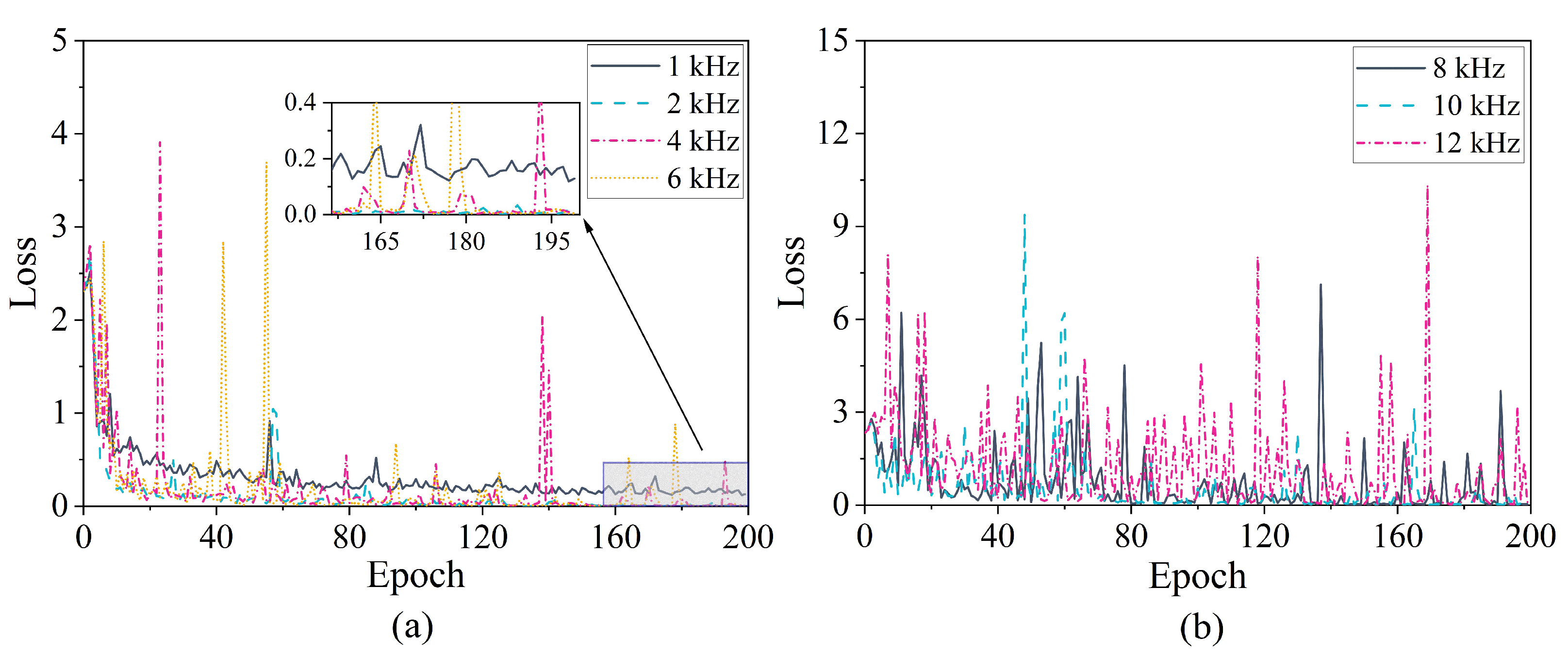
Machines 10 00282 g010
Figure 11. The validation loss of Dataset A (a) 1 kHz, 2 kHz, 4 kHz, and 6 kHz, (b) 8 kHz, 10 kHz, and 12 kHz.
Machines 10 00282 g011
Figure 12. The average accuracy and loss of different frequencies on dataset A.
Machines 10 00282 g012
Figure 13. The GAF images of Dataset A.
Machines 10 00282 g013
Figure 14. Comparison results between seven methods on dataset A.
Machines 10 00282 g014
Figure 15. Visualization of different diagnostic results on dataset A, (a) The proposed method, (b) GAF-SE-CNN, (c) GAF-CBAM-CNN, (d) GAF-BAM-CNN, (e) VMD-Gray image-Resnet50, (f) EMD-Gray image-Resnet50.
Machines 10 00282 g015
Figure 16. The confusion matrix of different diagnostic results on dataset A, (a) The proposed method, (b) GAF-SE-CNN, (c) GAF-CBAM-CNN, (d) GAF-BAM-CNN, (e) VMD-Gray image-Resnet50, (f) EMD-Gray image-Resnet50.
Machines 10 00282 g016
Figure 17. (a) Vertical view, (b) Front view, (c) SKF 6016-2RS1.
Machines 10 00282 g017
Figure 18. The validation accuracy of dataset B, (a) 1 kHz, 2 kHz, 4 kHz, (b) 5 kHz, 6 kHz, 8 kHz, and 10 kHz.
Machines 10 00282 g018
Figure 19. The validation loss of dataset B, (a) 1 kHz, 2 kHz, 4 kHz, (b) 5 kHz, 6 kHz, 8 kHz, and 10 kHz.
Machines 10 00282 g019
Figure 20. The accuracy and loss of dataset B.
Machines 10 00282 g020
Figure 21. The GAF images of dataset B.
Machines 10 00282 g021
Figure 22. Comparison results between seven methods on dataset B.
Machines 10 00282 g022
Figure 23. Visualization of different diagnostic results on dataset B, (a) The proposed method, (b) GAF-SE-CNN, (c) GAF-CBAM-CNN, (d) GAF-BAM-CNN, (e) VMD-Gray image-Resnet50, (f) EMD-Gray image-Resnet50.
Machines 10 00282 g023
Figure 24. The confusion matrix of different diagnostic results on dataset B, (a) The proposed method, (b) GAF-SE-CNN, (c) GAF-CBAM-CNN, (d) GAF-BAM-CNN, (e) VMD-Gray image-Resnet50, (f) EMD-Gray image-Resnet50.
Machines 10 00282 g024
Table 1. Dataset A: CWRU bearing operation states.
LabelFault Size (mm)StatesMotor Speed (r/min)Sample Size
1Normal (N)17971000 × 642 × 3
20.1778Inner race (IF1)17971000 × 642 × 3
30.1778Roll boll (RF1)17971000 × 642 × 3
40.1778Outer race (OF1)17971000 × 642 × 3
50.3556Inner race (IF2)17971000 × 642 × 3
60.3556Roll boll (RF2)17971000 × 642 × 3
70.3556Outer race (OF2)17971000 × 642 × 3
80.5334Inner race (IF3)17971000 × 642 × 3
90.5334Roll boll (RF3)17971000 × 642 × 3
100.5334Outer race (OF3)17971000 × 642 × 3
Table 2. Details of GAF-CA-CNN.
InputModuleUpOutputAttentionActivationSample Size
642 × 3Conv_block16HS2
322 × 16Bottleneck1616TrueRE2
162 × 16Bottleneck3624FalseRE2
82 × 24Bottleneck4424FalseRE1
82 × 24Bottleneck4840TrueHS2
42 × 40Bottleneck12040TrueHS1
42 × 40Bottleneck6048TrueHS1
42 × 48Bottleneck7248TrueHS1
42 × 48Bottleneck14496TrueHS2
22 × 96Bottleneck28896TrueHS1
22 × 96Conv_block288HS1
12 × 288Glob_avg_pool
12 × 512Conv2d512HS1
12 × 10Conv2d10Softmax1
Table 3. The average loss of Global Average Pool and Global Maximum Pool.
MethodsAverage Loss 1Average Loss 2Average Loss 3
GAF-CA-CNN-GAP0.1400.1940.158
GAF-CA-CNN-GMP0.1690.2370.182
Table 4. Parameter size and prediction speed of different models.
ModelsModel Size (MB)Prediction Speed (ms)
GAF-CA-CNN2.2060
GAF-SE-CNN2.3755
GAF-CBAM-CNN2.26104
GAF-BAM-CNN18.7113
VMD-Gray image-Resnet5090.571
EMD-Gray image-Resnet5090.578
Table 5. Diagnostics result of different methods on Dataset A.
Models12345AverageStandard Deviation
GAF-CA-CNN99.70%99.55%99.75%99.35%99.75%99.62%0.154
GAF-SE-CNN98.90%89.70%96.05%84.50%99.50%93.73%5.776
GAF-CBAM-CNN98.85%99.25%97.70%98.70%99.75%98.85%0.680
GAF-BAM-CNN99.05%96.05%98.45%99.65%97.95%98.23%1.230
VMD-Gray image-Resnet5091.25%91.75%94.75%87.50%86.50%90.35%3.002
EMD-Gray image-Resnet5095.33%94.67%95.00%98.33%98.33%96.33%1.637
Table 6. The parameters of SKF 6016-2RS1.
ParameterSize (mm)
d80
D125
B22
d1≈94.4
D2≈114.1
r1,2Min. 1.1
Table 7. Dataset B: Experiment bearing operation states.
LabelFault Size (mm)StatesMotor Speed (r/min)Sample Size
1Normal (N)5401000 × 642 × 3
2AbrasionRoll boll (RF1)5401000 × 642 × 3
3Single column pittingInner race (IF1)5401000 × 642 × 3
4Single column pittingOuter race (OF1)5401000 × 642 × 3
5Double column pittingInner race (IF2)5401000 × 642 × 3
6Double column pittingOuter race (OF2)5401000 × 642 × 3
73Inner race (IF3)5401000 × 642 × 3
83Outer race (OF3)5401000 × 642 × 3
96Inner race (IF4)5401000 × 642 × 3
106Outer race (OF4)5401000 × 642 × 3
Table 8. Diagnostics result of different methods on Dataset B.
Models12345AverageStandard Deviation
GAF-CA-CNN99.91%99.90%99.95%99.85%99.95%99.91%0.0371
GAF-SE-CNN99.95%98.75%96.54%99.55%97.25%98.41%1.3137
GAF-CBAM-CNN94.10%98.40%96.20%99.30%96.90%96.98%1.8059
GAF-BAM-CNN99.85%99.35%93.45%98.60%93.70%96.99%2.8176
VMD-Gray image-Resnet5067.75%75.25%68.50%70.00%74.50%71.20%3.0959
EMD-Gray image-Resnet5096.67%95.33%93.00%87.33%96.33%93.73%3.4484
Publisher’s Note: MDPI stays neutral with regard to jurisdictional claims in published maps and institutional affiliations.

