Dynamic Response and Synchronizing Characteristic for the Dual-Motor Driving System in Non-Inertial System

Abstract

As one of the typical propulsion systems of the new-energy vehicles (NEVs), the dual-motor driving system (DMDS) is installed and fixed on the bodywork and moves together with the bodywork in space, that is, the DMDS works in non-inertial systems. The previous researches on the DMDS are based on the assumption that the bodywork is stationary. In fact, since the DMDS moves with the bodywork, besides its own excitation forces, it is inevitably affected by the additional inertial terms (AITs) caused by the change in the operating state of the NEVs. In order to investigate the dynamic response and synchronizing characteristic of the DMDS under different motion forms of NEVs, the dynamic model of the DMDS in a non-inertial system is established, considering the permanent magnet synchronous motors (PMSMs), time-varying meshing stiffness and transmission error of gears. Subsequently, the expressions of the AITs are deduced under different non-inertial conditions. The translational motion and circular motion of the vehicle are selected to analyze the dynamic response and synchronizing characteristics of the DMDS in a non-inertial system. The results show that the acceleration has a significant influence on the displacement response of gears, torque and speed of PMSMs, but the torque synchronization and speed synchronization between PMSMs are minimally influenced by both the acceleration and the AITs. Meanwhile, the AITs that affect the displacement response are analyzed and quantified.

1. Introduction

It is generally believed that vehicles that use fossil fuels are one of the top sources of air pollution, and the depletion of oil is another serious problem that people have to face. As a consequence, new-energy vehicles (NEVs) are increasingly needed and have been listed as a development priority for all countries. Normally, the NEVs are driven by electric drive gear systems, such as the combination of a single motor or multiple motors with a gear transmission system. As one of the typical propulsion systems of NEVs, the dual-motor driving system (DMDS) has become the focus of more and more people, and has been reported in many literatures in the past. For example, Yang et al. designed a high power dual motor drive system to resolve the limitation of permanent magnet synchronous motor (PMSMs) application (such as temperature characteristics of permanent magnet materials and flux-weakening control problems) and utilize its good performances [1] and Tang provided a method and apparatus for optimizing the torque applied by each motor of a dual motor drive system of an all-electric vehicle [2]. In the traditional research on the dynamic response or synchronization property of DMDS, the DMDS is considered to be stationary relative to the earth reference system. In fact, the DMDS is installed and fixed on the bodywork, and moves together with the bodywork in space, that is, the DMDS operates in a non-inertial system. Besides its own excitation forces, the DMDS is inevitably affected by additional inertial forces and gyroscopic moments, which affects the dynamic response and synchronization property of DMDS. Therefore, the effects of non-inertia should be considered when the NEVs perform a spatial motion.

In the past few decades, many scholars across the world have carried out meaningful research on the combination of a single motor or multiple motors with a gear transmission system attached to a moving body, including modeling, dynamic response and synchronization property, etc. In modeling and dynamic property terms, Inalpolat et al. established a transverse-torsional dynamic mode of a spur gear reducer, including periodically time-varying meshing stiffness and nonlinearities caused by tooth separations in resonance regions, and the influence of gear tooth indexing errors on the dynamic response was investigated [3]. Giagopulos et al. proposed a dynamic model of a gear-pair system considering the gear backlash and bearing stiffness non-linearities, and then the effect of non-linearities in the identification and fault detection of gear-pair system were investigated [4]. Setiawan et al. developed a mathematical model for multispeed transmissions in electric vehicles, and the transient dynamic response of the transmission was studied. The established model was subsequently validated by comparing its results with experiment results [5]. Sun et al. developed a coupling dynamic model of a multi-motor gear system by employing the proposed hierarchical modeling method and obtained the influence rules of system parameters on the natural frequency. Meanwhile, dynamic behaviors under different load conditions were also obtained [6]. Liu et al. used the proposed hybrid user-defined element method to establish the dynamic model of a gear transmission system in an electric vehicle, and investigated the effect of meshing impact force and meshing stiffness on the dynamic behavior of the system [7]. Tang et al. established a novel torsional vibration dynamic model of a hybrid power train, and the effect of a dual-mass flywheel on the torsional vibration characteristics of a power-split hybrid power train was studied [8]. Zhang et al. established a multi-degree-of freedom (M-D-O-F) dynamic model of a two-stage gear set that included the time-variant stiffness and gear backlash feature, and then the nonlinear response of the two-stage gear set under the combined periodic and stochastic excitations was investigated [9]. Yan et al. presented a new design by integrating a planetary gear train (PGT) within a DC motor to form a compact structure assembly, and then investigated the effects of the gear tooth on the dynamic responses of the DC motor associated with the kinematics of the PGT [10]. Mashimo et al. proposed a micro geared ultrasonic motor and its dynamic model was established to analyze the dynamic characteristics [11]. Kim et al. proposed a dual actuator unit (DAU) composed of two actuators and a planetary gear train; the mathematic model of the DAU was developed to investigate the performance of position tracking, stiffness variation, etc. [12]. In addition, Lee et al. also proposed a similar actuator system using a planetary gear and two motors; subsequently, a dynamic model of the actuator system was established to analyze the output velocity and torque, and obtain frequency response characteristics [13]. In addition, regarding synchronization characteristics, Wei et al. established a coupling dynamic model of a multi-source driving transmission system considering the flexible shafts, support bearing and meshing gear pair; the speed and torque synchronization properties under an impact load at different load change rates were studied [14]. Zhao et al. investigated the real-time speed synchronization of multiple induction motors during load variation and speed acceleration [15]. Xiong et al. addressed the system dynamic response synchronization and real-time problems by employing a dynamic simulation test system for electric vehicles with a dual drive circuit [16]. Shi et al. investigated the coupling characteristics and synchronization of multi-motors by using the presented synchronization control algorithm for a multi-motor speed synchronous driving system. The algorithm was employed to control the motion of the electronic circuit axis and virtual transmission shaft. The results showed that it improved the running response speed and synchronization accuracy between the motors [17]. Yang et al. established a translation-torsion coupling dynamic model of a multi-motor torque coupling system; the influence of system speed synchronization performance and torque synchronization performance on the load sharing behavior of the system were discussed [18].

At present, the related research on the combination of a single motor or multiple motors with a gear transmission system attached to a moving body mainly focuses on the dynamic response and synchronizing characteristics under inertial conditions, while related research under non-inertial conditions has rarely been reported. In fact, the gear transmission system is installed and fixed on the moving body and moves with the moving body. Obviously, under non-inertial conditions, the gear transmission system is not only affected by its own excitation forces, but is also affected by the additional inertial forces generated by the change in the operating state of the moving body. Therefore, it is necessary and meaningful to investigate the dynamic response and synchronizing characteristics of the combination of a single motor or multiple motors with a gear transmission system attached to a moving body. This paper will take the DMDS installed on the NEVs as an example to carry out the related research, and the organization of the paper is as follows. In Section 2, the dynamic model of DMDS in a non-inertial system is introduced. Then, the response and synchronizing characteristic of the DMDS under the translational motion and circular motion, two typical forms of NEV motion, are discussed in Section 3. Finally, some conclusions are drawn in Section 4.

2. Dynamic Model of Dual-Motor Driving System in Non-Inertial System

The DMDS, as shown in Figure 1, is composed of PMSMs, pinions and a bull wheel, etc. The two pinions are driven by two PMSMs (the rated power of each one is 100 kW) separately and the wheel is driven by the two pinions together; the shaft is connected to the wheel via the spline. Based on the finite element theory, the DMDS can be divided into the following four basic coupling elements: meshing element, shafting element, connecting element and bearing element. The dynamic model and node diagram of DMDS are shown in Figure 2.

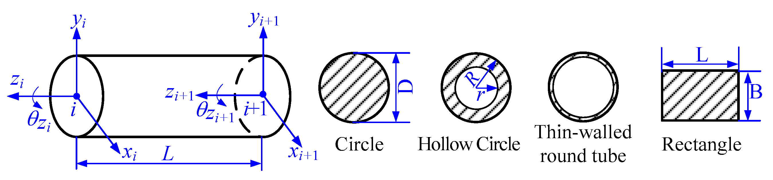
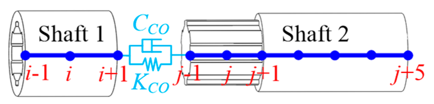
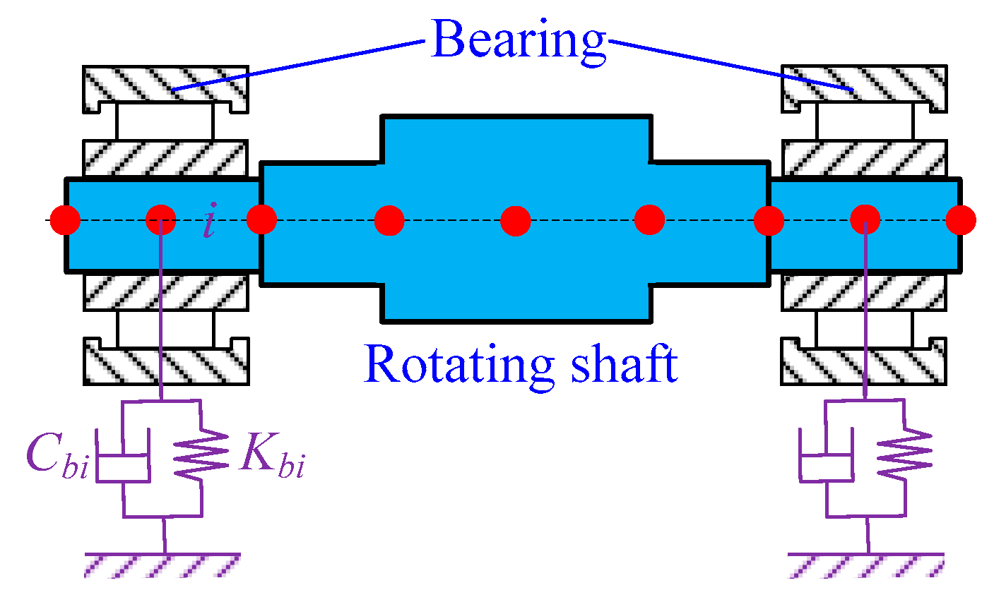
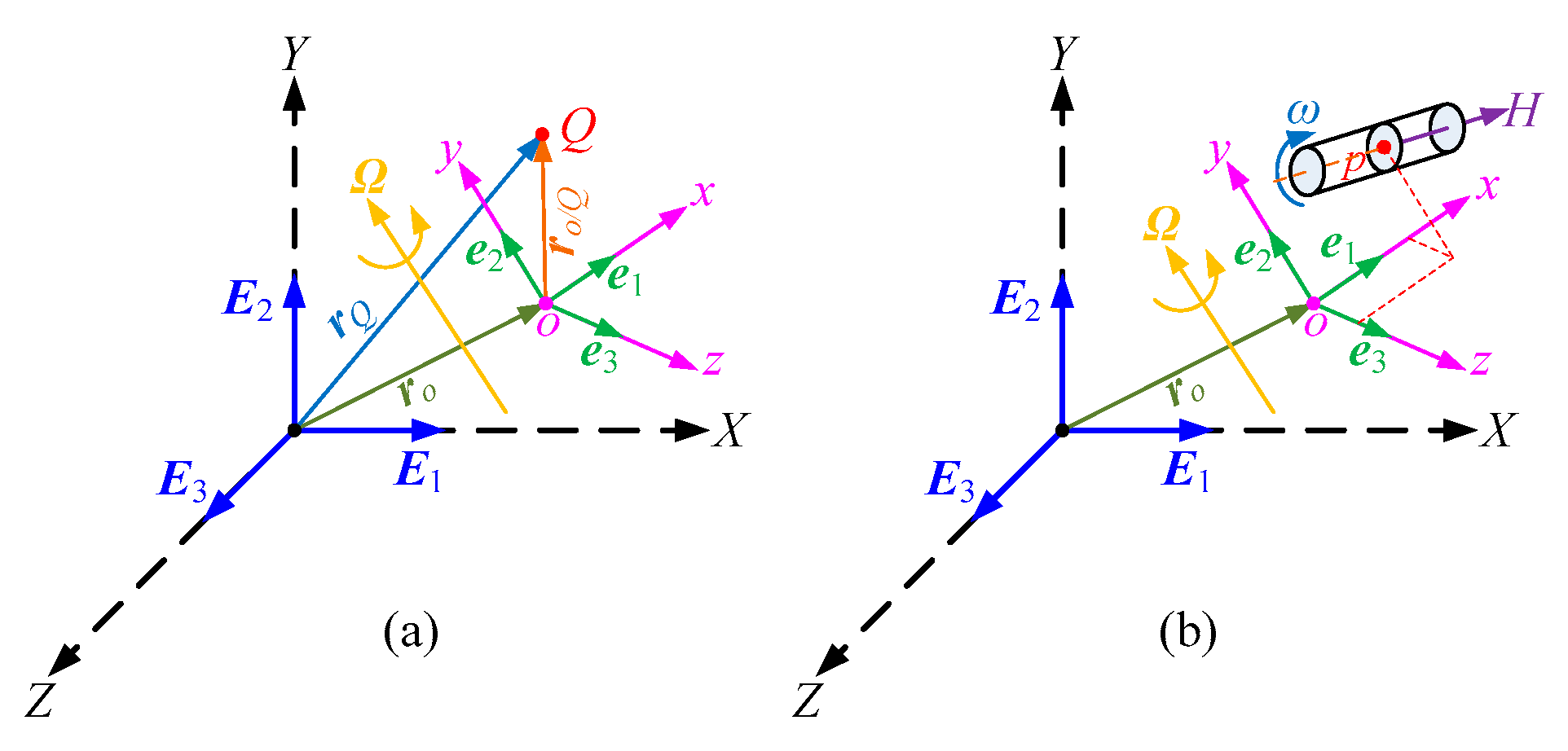
2.1. Dynamic Model of Basic Coupling Elements

Meshing elements. The meshing elements can be regarded as a bridge to couple two or more rotating shafts together and transmit motion and force, and can be described by a pair of rigid disks connected by a stiffness-damping spring system on the plane of action, as shown in Figure 3. φ, β and α are the relative position angle, helix angle and pressure angle of gears, respectively. r_p and r_g are the base radius of gear p and gear g, respectively. k_m is the meshing stiffness, which can be represented by rectangular ware and regarded as the time-varying function of gear rotational angular displacement, as shown in Figure 4. e_m and c_m are the transmission error and meshing damping, respectively, and they are the time-varying variables. Herein, e_m can be solved by referring to Ref. [18] and viewed as the time-varying function of gear rotational angular displacement. Therefore, the time-varying variables k_m, c_m and e_m can be expressed as Equation (2). x_i, y_i and z_i (i = p and g) are the horizontal, vertical and axial direction displacements of gears, respectively. θ_i (i = xp, yp and xg, yg) is the swing angular displacement of gears around the x-axis or y-axis, θ_j (j = zp and zg) is the rotational angular displacement of gears around the z-axis. The dynamic model of the meshing elements can be expressed as

$${\mathbf{M}}_{pg}{\ddot{\mathbf{X}}}_{pg}+{\mathbf{C}}_{pg}{\dot{\mathbf{X}}}_{pg}+{\mathbf{K}}_{pg}{\mathbf{X}}_{pg}={\mathbf{F}}_{pg}$$

(1)

where

$$\{\begin{array}{l}{\mathbf{M}}_{pg}=diag[m_p{m}_p{m}_p{I}_{xp}{I}_{yp}{I}_{zp}{m}_g{m}_g{m}_g{I}_{xg}{I}_{yg}{I}_{zg}]; {\mathbf{X}}_{pg}={[x_p{y}_p{z}_p{\theta }_{xp}{\theta }_{yp}{\theta }_{zp}{x}_g{y}_g{z}_g{\theta }_{xg}{\theta }_{yg}{\theta }_{zg}]}^T\\ {\mathbf{K}}_{pg}=k_m{\mathbf{V}}_{pg}^T{\mathbf{V}}_{pg};{\mathbf{F}}_{pg}=(k_m{e}_m+c_m{\dot{e}}_m){\mathbf{V}}_{pg}^T;{\mathbf{C}}_{pg}=c_m{\mathbf{V}}_{pg}^T{\mathbf{V}}_{pg}\\ {\mathbf{V}}_{pg}=[\cos \beta \sin (\alpha -\phi ),\cos \beta \cos (\alpha -\phi ),\sin \beta ,-r_p\sin \beta \sin (\alpha -\phi ),-r_p\sin \beta \cos (\alpha -\phi ),r_p\cos \beta ,\cdots \\ \hspace{1em}\hspace{1em}-\cos \beta \sin (\alpha -\phi ),-\cos \beta \cos (\alpha -\phi ),-\sin \beta ,-r_g\sin \beta \sin (\alpha -\phi ),-r_g\sin \beta \cos (\alpha -\phi ),-r_g\cos \beta ]\end{array}$$

M_pg, C_pg and K_pg are the mass, damping and stiffness matrices of the gear pair, respectively. X_pg and V_pg are the displacement vector and meshing matrix of the gear pair. F_pg is the exciting force vector, which is a non-constant vector and is related to the time-varying variables k_m, c_m and e_m.

$$\{\begin{array}{l}{k}_m={\overline{k}}_{pg}+{\displaystyle \sum _{l=1}^7{\widehat{k}}_{pgl}}\cdot \cos (\frac{l\cdot 2\pi \cdot r_p\cdot {\theta }_p}{p_{bp}}+{\gamma }_i)\\ c_m=2\xi \sqrt{k_m/(1/m_{eq,1}+1/m_{eq,2})}\\ e_m={\overline{e}}_{pg}+{\displaystyle \sum _{l=1}^7{\widehat{e}}_{pgl}}\cdot \cos (\frac{l\cdot 2\pi \cdot r_p\cdot {\theta }_p}{p_{bp}}+{\gamma }_i)\end{array}$$

(2)

where ${\widehat{k}}_{pgl}$ and ${\overline{k}}_{pg}$ are the lth harmonic term amplitude and mean mesh stiffness, respectively. ${\widehat{e}}_{pgl}$ and ${\overline{e}}_{pg}$ are the lth harmonic term amplitude and mean transmission error, respectively. γ_i is the phase angle. θ_p and p_bp denote the rotational angular displacement around the z-axis of gear p, and the base pitch of gear p, respectively. ξ is the damping ratio. m_eq,1 and m_eq,2 are the equivalent qualities of the gears.

Shafting elements. The rotating components (such as shafts and gears) of the DMDS can be equivalent to the shafting elements with different cross sections, including hollow circle cross-section, circle cross-section, etc. The force state and deformation state of the shafting elements can be analyzed by employing the Timoshenko beam theory [19,20], as shown in Figure 5. The deformation of the shafting elements can be described by the displacement of the nodes and the dynamic model of the two-node shafting element can be express as

$${\mathbf{M}}_{i,i+1}{\ddot{\mathbf{X}}}_{i,i+1}+{\mathbf{C}}_{i,i+1}{\dot{\mathbf{X}}}_{i,i+1}+{\mathbf{K}}_{i,i+1}{\mathbf{X}}_{i,i+1}=\mathbf{0}$$

(3)

M_i,i+1 and X_i,i+1 are the mass matrix and displacement vector, respectively. K_i,i+1 is the stiffness matrix with a 12 × 12 order form and can be solved by referring to Ref. [20]. C_i,i+1 is the damping matrix and can be solved by Rayleigh damping, C_i,i+1 = λ₁M_i,i+1 + λ₂K_i,i+1, where λ₁ and λ₂ represent the proportionality coefficients.

Connecting elements. The connecting elements can be employed to describe the coupling relationship between two connecting components, such as couplings and splines. For example, as shown in Figure 6, the coupling relationship between nodes i on the internal spline and node j on the external spline can be described by means of a spring-damper system. Therefore, the dynamic model of the connecting elements can be expressed as

$$\left[\begin{array}{cc}{\mathbf{M}}_i& \mathbf{O}\\ \mathbf{O}& {\mathbf{M}}_j\end{array}\right]\left[\begin{array}{c}{\ddot{\mathbf{X}}}_i\\ {\ddot{\mathbf{X}}}_j\end{array}\right]+\left[\begin{array}{cc}{\mathbf{C}}_{co}& -{\mathbf{C}}_{co}\\ -{\mathbf{C}}_{co}& {\mathbf{C}}_{co}\end{array}\right]\left[\begin{array}{c}{\dot{\mathbf{X}}}_i\\ {\dot{\mathbf{X}}}_j\end{array}\right]+\left[\begin{array}{cc}{\mathbf{K}}_{co}& -{\mathbf{K}}_{co}\\ -{\mathbf{K}}_{co}& {\mathbf{K}}_{co}\end{array}\right]\left[\begin{array}{c}{\mathbf{X}}_j\\ {\dot{\mathbf{X}}}_j\end{array}\right]=\mathbf{0}$$

(4)

M_i and M_j are the mass matrices of nodes i and j, respectively. X_i and X_j represent the displacement vectors of nodes i and j, respectively. K_co and C_co are the coupling stiffness and damping matrices between the internal and external splines, respectively.

Bearing elements. The bearings are used to support the rotating shafts and constrain its horizontal and vertical movement, which can be equivalent to a spring-damper system, as shown in Figure 7. K_bi is the support stiffness matrix of the support node i on the rotating shaft, and the Ref. [21] can be referred to in order to provide the specific form of K_bi. C_bi represents the support damping matrix of the support node i on the rotating shaft, and C_bi has the same structure as K_bi. The dynamic model of the bearing element’s corresponding support node i on the rotating shaft can be expressed as

$${\mathbf{M}}_{bi}{\ddot{\mathbf{X}}}_{bi}+{\mathbf{C}}_{bi}{\dot{\mathbf{X}}}_{bi}+{\mathbf{K}}_{bi}{\mathbf{X}}_{bi}=\mathbf{0}$$

(5)

X_bi and M_bi represent the displacement vector and mass matrix of the support node i on the rotating shaft, respectively.

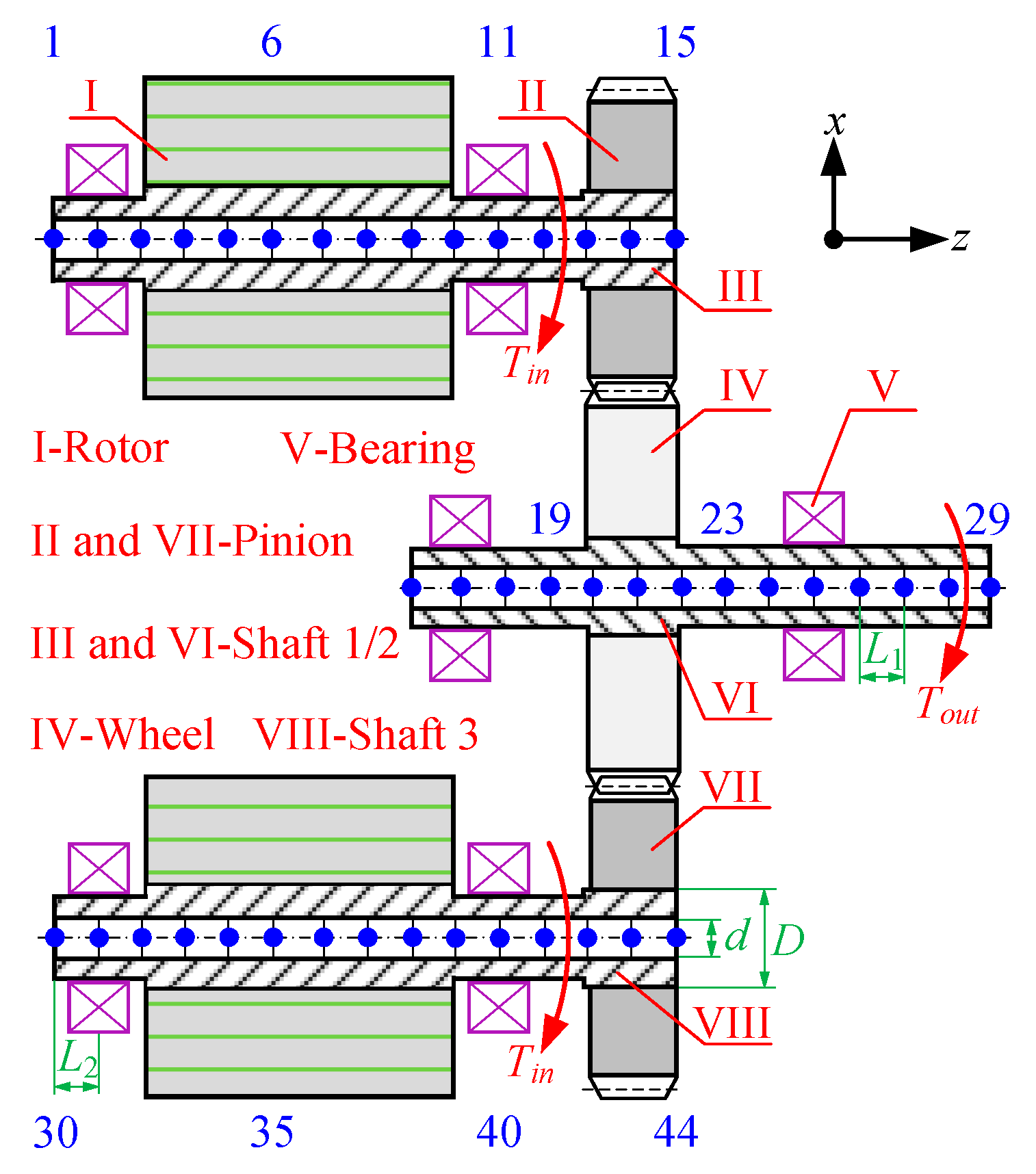
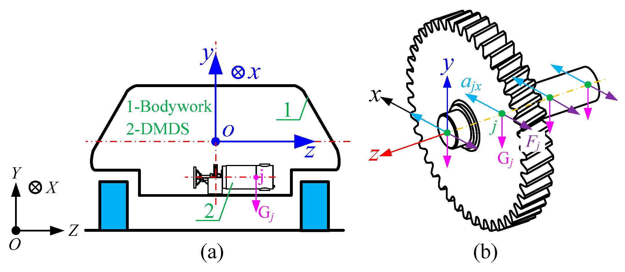
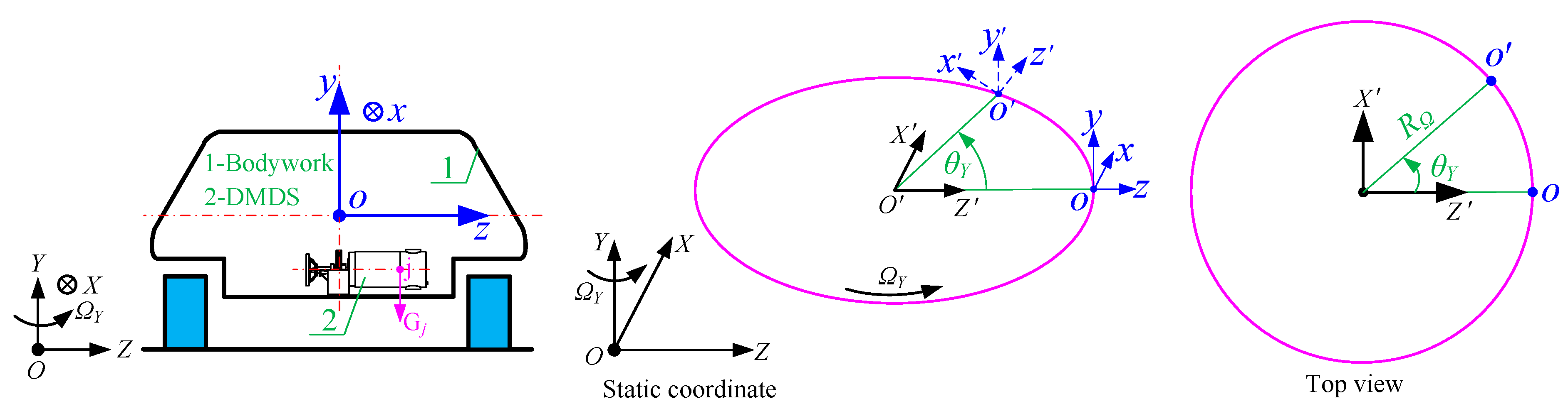
2.2. Dynamic Model of Dual-Motor Driving System in Non-Inertial System

The rotating shafts of the DMDS are simulated by the shafting elements, and they can be assembled together by means of the meshing elements, connecting elements and bearing elements according to the node distribution diagram illustrated in Figure 2. The coupling matrix assemble method described in the Ref. [21] can be used to establish the overall system dynamic model of DMDS, which contains 44 nodes. The overall system dynamic model can be expressed as

$$\mathbf{M}\ddot{\mathbf{X}}(\mathrm{t})+\mathbf{C}(\mathrm{t})\dot{\mathbf{X}}(\mathrm{t})+\mathbf{K}(\mathrm{t})\mathbf{X}(\mathrm{t})=\mathbf{F}(\mathrm{t})+\mathbf{G}(\mathrm{t})+\mathbf{M}(\mathrm{t})+\mathbf{T}(\mathrm{t})$$

(6)

M and X(t) are the overall mass matrix and displacement vector, and their dimensions are 264 × 264 and 264 × 1, respectively. C(t) and K(t) represent the overall damping and stiffness matrices, and the dimensions of these matrices are 264 × 264, respectively. F(t), G(t) and M(t) and T(t) are the additional inertial force vector, gravity and gyroscopic moment vector and external load excitation vector, and the dimensions of these vectors are 264 × 1, respectively. T(t) can be expressed as

$$\mathbf{T}(\mathrm{t})={[0,0,0,0,0,0,\cdots ,\underset{\mathrm{p}\mathrm{o}\mathrm{w}\mathrm{e}\mathrm{r}\mathrm{i}\mathrm{n}\mathrm{p}\mathrm{u}\mathrm{t}\mathrm{n}\mathrm{o}\mathrm{d}\mathrm{e}6}{\underbrace{0,0,0,0,0,T_{in}}},\cdots ,\underset{\mathrm{n}\mathrm{o}\mathrm{d}\mathrm{e}i}{\underbrace{0,0,0,0,0,0}},\cdots ,\underset{\mathrm{p}\mathrm{o}\mathrm{w}\mathrm{e}\mathrm{r}\mathrm{o}\mathrm{u}\mathrm{p}\mathrm{u}\mathrm{t}\mathrm{n}\mathrm{o}\mathrm{d}\mathrm{e}28}{\underbrace{0,0,0,0,0,T_{out}}},\cdots ,\underset{\mathrm{p}\mathrm{o}\mathrm{w}\mathrm{e}\mathrm{r}\mathrm{i}\mathrm{n}\mathrm{p}\mathrm{u}\mathrm{t}\mathrm{n}\mathrm{o}\mathrm{d}\mathrm{e}35}{\underbrace{0,0,0,0,0,T_{in}}},\cdots ,\underset{\mathrm{n}\mathrm{o}\mathrm{d}\mathrm{e}N}{\underbrace{0,0,0,0,0,0}}]}^T$$

(7)

T_out is the load torque that acts on the power output node. T_in is the output torque of PMSMs that acts on the power input node. T_in can be obtained by establishing the simulation model of PMSMs, and the modeling process is described in detail in Ref. [22], and the key parameters of PMSMs are listed in

Table 1. Key parameters of PMSMs.

	Stator	Rotor	Unit
Resistance	8.296 × 10−3	7.11 × 10−2	Ω
Rated speed	—	2400	rpm
Rated voltage	540	—	VDC
Leakage inductance	5.05 × 10−5	5.05 × 10−5	H
Rotational inertia	—	8.86 × 10−1	kg·m2
Magnetizing inductance	8.49 × 10−5	8.49 × 10−5	H
Dimensions	φ380 × L399		mm
Mass	130		kg
Rated power	100		kW
Rated torque	400		Nm

.

Additional force and moment. The DMDS is installed and fixed to the bodywork and moves together with the bodywork in space. Therefore, the effects of non-inertia on the DMDS operating in moving bodywork should be considered, and the thermal changes between PMSM and the gear transmission system is ignored. As shown in Figure 8a, a non-inertial system is employed to describe the absolute motion of point Q in space, where OXYZ is a static coordinate system fixed on earth, and oxyz is a moving coordinate system that is relative to the OXYZ and fixed on moving bodywork. E_i and e_i (i = 1, 2 and 3) are the base vectors of OXYZ and oxyz, respectively. r_o and r_Q are the position vectors of origin o and moving point Q, respectively and they are measured in OXYZ. r_o/Q is the relative position vector of moving point Q, which is measured in oxyz. Ω is the angular velocity vector of oxyz and measured in OXYZ. The position vector r_Q can be expressed as

$${\mathit{r}}_Q={\mathit{r}}_o+{\mathit{r}}_{o/Q}=X_o{\mathit{E}}_1+Y_o{\mathit{E}}_2+Z_o{\mathit{E}}_3+x_Q{\mathit{e}}_1+y_Q{\mathit{e}}_2+z_Q{\mathit{e}}_3$$

(8)

where X_o, Y_o, Z_o and x_Q, y_Q, z_Q are the variables. E_i and e_i (i = 1, 2 and 3) are the constant vector and variable vector, respectively. The absolute velocity vector v_Q can be obtained by taking the derivative of the position vector r_Q with respect to time, and it can be expressed as

$$\{\begin{array}{l}{\mathit{v}}_Q=\frac{d{\mathit{r}}_Q}{dt}={\dot{X}}_o{\mathit{E}}_1+{\dot{Y}}_o{\mathit{E}}_2+{\dot{Z}}_o{\mathit{E}}_3+{\dot{x}}_Q{\mathit{e}}_1+{\dot{y}}_Q{\mathit{e}}_2+{\dot{z}}_Q{\mathit{e}}_3+x_Q\frac{d{\mathit{e}}_1}{dt}+y_Q\frac{d{\mathit{e}}_2}{dt}+z_Q\frac{d{\mathit{e}}_3}{dt}\\ ={\mathit{v}}_o+{\mathit{v}}_{o/Q}+\mathit{\Omega }\times {\mathit{r}}_{o/Q}\\ \frac{d{\mathit{e}}_i}{dt}=\mathit{\Omega }\times {\mathit{e}}_i,i=1,2\mathrm{a}\mathrm{n}\mathrm{d}3\end{array}$$

(9)

Then, the absolute acceleration vector a_Q can be obtained by taking the derivative of the absolute velocity vector v_Q with respect to time, and it can be expressed as

$$\{\begin{array}{l}{\mathit{a}}_Q=\frac{d{\mathit{v}}_Q}{dt}={\mathit{a}}_o+\frac{d{\mathit{v}}_{o/Q}}{dt}+\frac{d\mathit{\Omega }}{dt}\times {\mathit{r}}_{o/Q}+\mathit{\Omega }\times \frac{d{\mathit{r}}_{o/Q}}{dt}={\mathit{a}}_o+{\mathit{a}}_{o/Q}+\dot{\mathit{\Omega }}\times {\mathit{r}}_{o/Q}+2\mathit{\Omega }\times {\mathit{v}}_{o/Q}+\mathit{\Omega }\times (\mathit{\Omega }\times {\mathit{r}}_{o/Q})\\ \frac{d{\mathit{r}}_{o/Q}}{dt}={\dot{x}}_Q{\mathit{e}}_1+{\dot{y}}_Q{\mathit{e}}_2+{\dot{z}}_Q{\mathit{e}}_3+x_Q\frac{d{\mathit{e}}_1}{dt}+y_Q\frac{d{\mathit{e}}_2}{dt}+z_Q\frac{d{\mathit{e}}_3}{dt}\end{array}$$

(10)

(1) When the NEVs perform a variable speed translational motion, from Equation (10), it can be observed that the absolute acceleration term of the moving point Q can be derived as a_Q = a_o + a_o/Q, where a_o is the convected acceleration term and a_o/Q is the relative acceleration term. Since there is no relative movement between DMDS and the bodywork, this means that a_o/Q = 0. Therefore, when the NEVs perform a variable speed translational motion, the additional inertial force term F(t) can be expressed as

$$\mathbf{F}(\mathrm{t})=-m_i\cdot {\mathit{a}}_{i/o}=-m_i\cdot {[\underset{\mathrm{n}\mathrm{o}\mathrm{d}\mathrm{e}1}{\underbrace{a_{1x/o},a_{1y/o},a_{1z/o},0,0,0}},\cdots ,\underset{\mathrm{n}\mathrm{o}\mathrm{d}\mathrm{e}i}{\underbrace{a_{ix/o},a_{iy/o},a_{iz/o},0,0,0}},\cdots ,\underset{\mathrm{n}\mathrm{o}\mathrm{d}\mathrm{e}N}{\underbrace{a_{Nx/o},a_{Ny/o},a_{Nz/o},0,0,0}}]}^T$$

(11)

where m_i is the mass of node i on the rotating shaft, and a_i/o (i = 1, 2, …, N) represents the convected acceleration vector of node i on the rotating shaft and is measured in OXYZ. a_ix/o, a_iy/o and a_iz/o are the components of a_i/o in x, y and z directions, respectively. Besides F(t), the node i on the rotating shaft is also affected by gravity G(t), and it can be expressed as

$$\mathbf{G}(\mathrm{t})=-m_i\cdot {\mathit{a}}_{ig}=-m_i\cdot {[\underset{\mathrm{n}\mathrm{o}\mathrm{d}\mathrm{e}1}{\underbrace{a_{1gx},a_{1gy},a_{1gz},0,0,0}},\cdots ,\underset{nodei}{\underbrace{a_{igx},a_{igy},a_{igz},0,0,0}},\cdots ,\underset{\mathrm{n}\mathrm{o}\mathrm{d}\mathrm{e}N}{\underbrace{a_{Ngx},a_{Ngy},a_{Ngz},0,0,0}}]}^T$$

(12)

where a_ig (i = 1, 2, …, N) represents the gravitational acceleration vector of node i on the rotating shaft. a_igx, a_igy and a_igz are the components of a_ig in x, y and z directions, respectively.

(2) When the NEVs performs a variable speed circular motion, from Equation (10), the absolute acceleration term of moving point Q can be derived as follows: a_Q = a_o/Q + ×r_o/Q + Ω × (Ω × r_o/Q) + 2Ω × v_o/Q, where $\dot{\mathit{\Omega }}$ × r_o/Q and Ω × (Ω × r_o/Q) are the first convected acceleration term and second convected acceleration term, respectively, and are denoted as a_r1 and a_r2, respectively. Herein, a_r = a_r1 + a_r2. 2Ω × v_o/Q is the Coriolis acceleration term and is denoted as a_c. Similarly, since there is no relative movement between DMDS and the bodywork, the relative acceleration term a_o/Q = 0. Thus, when the NEVs performs a variable speed circular motion, the additional inertial force term F(t) can be expressed as

$$\begin{array}{l}\mathbf{F}(\mathrm{t})=-m_i\cdot ({\mathit{a}}_{ir}+{\mathit{a}}_{ic})=-m_i\cdot [\underset{\mathrm{n}\mathrm{o}\mathrm{d}\mathrm{e}1}{\underbrace{a_{1rx}+a_{1cx},a_{1ry}+a_{1cy},a_{1rz}+a_{1cz},0,0,0}},\cdots ,\\ \underset{\mathrm{n}\mathrm{o}\mathrm{d}\mathrm{e}i}{\underbrace{a_{irx}+a_{icx},a_{iry}+a_{icy},a_{irz}+a_{icz},0,0,0}},\cdots ,\underset{\mathrm{n}\mathrm{o}\mathrm{d}\mathrm{e}N}{\underbrace{a_{Nrx}+a_{Ncx},a_{Nry}+a_{Ncy},a_{Nrz}+a_{Ncz},0,0,0}}{]}^T\end{array}$$

(13)

where a_ir and a_ic (i = 1, 2, …, N) represent the convected acceleration and Coriolis acceleration vectors of node i on the rotating shaft, respectively. a_irx, a_iry, a_irz and a_icx, a_icy, a_icz are the components of a_ir and a_ic in x, y and z directions, respectively. The gravity term G(t) can be calculated by Equation (12). Moreover, the rotating shaft will be subjected to an additional gyroscopic moment, due to the rotating angular velocity ω when the NEVs perform a circular motion. As shown in Figure 8b, the moment of momentum can be described as H = J·ω and J is the polar moment of inertia. Hence, under the interaction of Ω and ω, the additional gyroscopic moment M(t) can be expressed as

$$\begin{array}{l}\mathbf{M}(\mathrm{t})=\mathbf{H}\times \mathit{\Omega }=J\cdot \omega \times \mathit{\Omega }=[\underset{\mathrm{n}\mathrm{o}\mathrm{d}\mathrm{e}1}{\underbrace{0,0,0,J_{1x}{\omega }_{1x}{\Omega }_{1x},J_{1y}{\omega }_{1y}{\Omega }_{1y},J_{1z}{\omega }_{1z}{\Omega }_{1z}}},\cdots ,\\ \underset{\mathrm{n}\mathrm{o}\mathrm{d}\mathrm{e}i}{\underbrace{0,0,0,J_{ix}{\omega }_{ix}{\Omega }_{ix},J_{iy}{\omega }_{iy}{\Omega }_{iy},J_{iz}{\omega }_{iz}{\Omega }_{iz}}},\cdots ,\underset{\mathrm{n}\mathrm{o}\mathrm{d}\mathrm{e}N}{\underbrace{0,0,0,J_{Nx}{\omega }_{Nx}{\Omega }_{Nx},J_{Ny}{\omega }_{Ny}{\Omega }_{N\mathrm{y}},J_{Nz}{\omega }_{Nz}{\Omega }_{Nz}}}{]}^T\end{array}$$

(14)

J_ij and ω_ij (j = x, y and z) are the moment of inertia and angular velocity of node i around the j-axis, respectively, and Ω_ij (j = x, y and z) is the angular velocity of node i around the axes other than the j-axis.

3. Dynamic Response and Synchronizing Characteristic Analysis in Non-Inertial System

The software MATLAB/Simulink (license: 40927247) is used to build the simulation model of the DMDS, and the translational motion and circular motion of the NEVs are selected to investigate the response and synchronizing characteristics of the DMDS in a non-inertial system. The key parameters of the DMDS are listed in

Table 2. Key parameters of DMDS.

Parameters	Values	Parameters	Values
Tooth number (pinion/wheel)	23/69	Length of shaft 1 (or 3) L1 (mm)	32
Module (mm)	4	Diameter of shaft 2 D/d (mm)	65/45
Width (mm)	35	Length of shaft 2 L2 (mm)	20
Pressure angle α (°)	20	Bearing translational stiffness (Nm−1)	kx = ky = 1.2 × 108; kz = 9.5 × 107
Helix angle β (°)	15	Bearing torsional stiffness (Nm−1)	kθx = kθy = 1.0 × 107
Diameter of shaft 1 (or 3) D/d (mm)	60/45	Transmission error amplitude (µm)	20

.

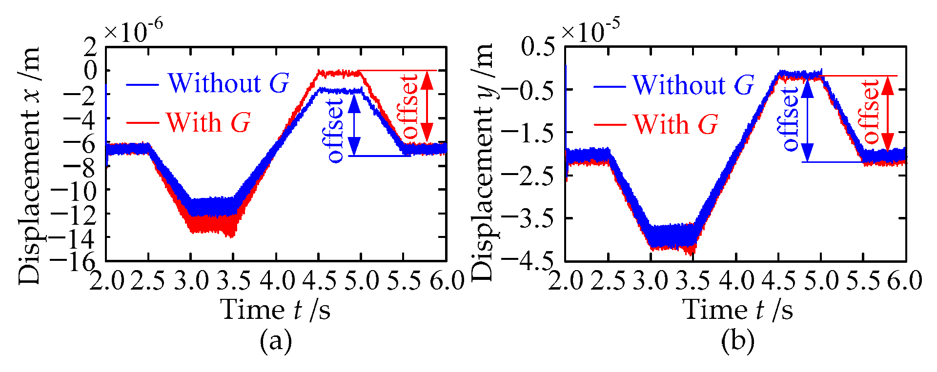
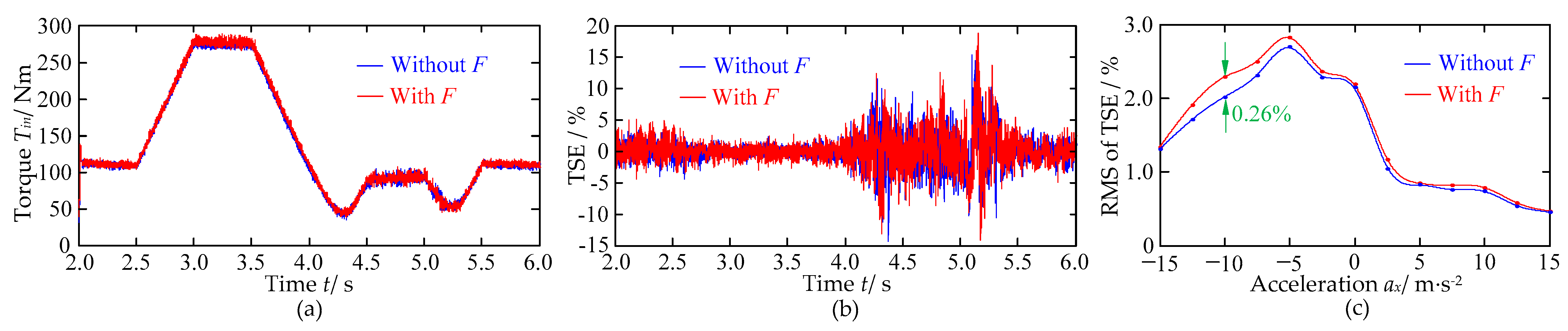
3.1. Case I: The NEVs Perform a Variable Speed Translational Motion

If one supposes that the NEVs travel in a straight line with variable speed in the x-direction, the force condition is shown as Figure 9, and the basic parameters of NEVs are listed in

Table 3. Basic parameters of NEVs.

Parameters	Values	Parameters	Values	Parameters	Values
Length (mm)	4675	High (mm)	1500	Front/rear track (mm)	1525/1520
Width (mm)	1770	Wheelbase (mm)	2670	Weight (kg)	1531

. For the gravity of node j, G_j = −m_j·a_g·(0·e₁ + e₂ + 0·e₃), as shown in Figure 9a. For the additional convected inertial force (ACIF) of node j, F_j = −m_j·a_jx·(e₁ + 0·e₂ + 0·e₃), as shown in Figure 9b. The total gravity and ACIF of a shaft are equal to the sum of G_j and F_j of all the nodes on the shaft, respectively.

The curves of the translation acceleration a_x and translational speed v in the x-direction shown in Figure 10 are employed to investigate the response and synchronizing characteristics of the DMDS under different non-inertial conditions. The initial translational speed of the vehicle is 80 km/h and the rotating speeds of PMSMs are 1900 rpm, and the load imposed on the DMDS is 600 Nm. If one takes as an example the displacement responses of node 14 (gear node) under different non-inertial conditions, as shown in Figure 11, it can be clearly observed that the displacement response curves in the x- and y-directions are significantly associated with the a_x-t curve; the difference between both of them is that they exhibit a full reversal. The displacement responses increase with the increase in a_x, but the magnitude in the y-direction is markedly greater than that in the x-direction.

According to the theoretical analysis, when the NEVs perform a translational motion, the nodes are not only affected by the torque of PMSMs (T_in), but also by ACIF (F) in the x-direction and gravity (G) in the y-direction. Figure 12a shows the displacement responses with or without F when a_x changes from 10 to −10 m·s⁻². As a consequence, the offset of the red line is significantly greater than that of blue line. Similarly, due to the effect of gravity G, the offset of the displacement response in the y-direction has increased, but is not obvious, as shown in Figure 12b.

In addition, the relative influence proportion γ_i is used to analyze the degree of influence of F or G on the displacement response, and it can be calculated by Equation (15). As shown in Figure 13a, the influence of F on the displacement response in the x-direction is obviously greater than that of G on the displacement response in the y-direction. When a_x changes from −15 to 15 m·s⁻², the relative influence proportion of F has a numerically negative correlation with a_x, and then has a numerically positive correlation with a_x. When a_x = −15 or 15 m·s⁻², the relative influence proportion reaches the maximum value, which is about 24%. However, when a_x changes from −15 to 15 m·s⁻², the relative influence proportion of G has a numerically positive correlation with a_x, and then has a numerically negative correlation with a_x, and the maximum relative influence proportion only reaches 2.3% when a_x = 0 m·s⁻², as shown in Figure 13b. Therefore, the gravity G is not the primary influence factor, and its influence can be ignored whether it is in inertial or non-inertial conditions.

$${\gamma }_i=({\delta }_i-{\delta }_t)/{\displaystyle \sum ({\delta }_i-{\delta }_t)}\times 100\%$$

(15)

δ_i is the offset when the factor i is not considered and δ_t is the offset when all factors are considered.

The vibration of gears can be transmitted to the PMSMs and affect the torque and speed of PMSMs. Considering that the gravity G has very little effect on the displacement responses of gears, we next focus on the effect of ACIF on the torque and speed of PMSMs. Herein, the synchronization error (SE) is applied to measure the synchronization of the output variables (torque and speed) between PMSMs. The greater the SE, the greater the difference in the output variables between PMSMs, which can be expressed as

$$E_{\lambda }=\frac{{({\lambda }_l-{\lambda }_{mean})}_{\max }}{{\lambda }_{mean}}\times 100\%,{\lambda }_{mean}=\frac{1}{N}{\displaystyle \sum _{i=1}^N{\lambda }_l}$$

(16)

E_λ is the SE, λ = T_in and v, l = 1, 2, …, N. T_in and v represent the torque and speed of PMSMs, respectively. N is the number of PMSMs and N = 2 in this study.

The torque of PMSMs and its torque synchronization error (TSE) are shown in Figure 14. Except for the fact that there is some fluctuation at 4.0–4.5 s and 5.0–5.5 s, the curve of torque is very close to the a_x–t curve, as shown in Figure 14a. Obviously, the torque remains almost unchanged before and after considering the ACIF. Similarly, the TSE between PMSMs has hardly changed, and their amplitudes fluctuate between −2.1% and 2.3% during acceleration and fluctuate between −14.2% and 18.8% during deceleration. This phenomenon is firstly because the growth of the numerator in Equation (16) is lesser than that of the denominator, and second because the mean value of torque (namely, λ_mean) during acceleration is significantly greater than that during deceleration. Figure 14c shows the curve of the root mean square (RMS) value of TSE. When a_x changes in the range of −15 to 15 m·s⁻², with the decrease in the numerical value of a_x, the RMS value of TSE increases and then decreases and the maximum value appears when a_x = −2.5 m·s⁻² and is about 2.8%. The reason for this is that the torque of PMSMs is at its minimum value when a_x = −2.5 m·s⁻², namely when λ_mean in Equation (16) is at its minimum value, so the calculated E_λ is at its maximum value. It indicates that the change in translation acceleration has a small effect on the synchronization of torque between PMSMs. Moreover, through the analysis and comparison, it is found that the change in the RMS value of TSE is minor before and after considering the ACIF, and the maximum difference between the two is only 0.26%, indicating that the ACIF also has a small effect on the synchronization of torque between PMSMs.

The speed of PMSM and its speed synchronization error (SSE) are shown in Figure 15. The curve of speed exhibits good correlation with the v–t curve, as shown in Figure 15a. There is no obvious change in speed at any of the times, regardless of whether the ACIF is considered or not. This can also be verified by Figure 15b and compared with the case without considering F, the change in SSE is not noticeable, and its amplitude fluctuates between −2.2‰ and 2.3‰. In addition, the curve of the RMS value of SSE under different translation acceleration conditions is plotted, as shown in Figure 15c. When a_x changes in the range of −15 to 15 m·s⁻², with the decrease in the numerical value of a_x, the RMS value of SSE increases and then decreases and the maximum value appears when a_x = −0 m·s⁻² and is about 5.03‰. This is because the speed of PMSMs is at its minimum value when a_x = 0 m·s⁻², namely when λ_mean in Equation (16) is at its minimum value, so the calculated E_λ is at its maximum value. This means that the changes in a_x have a small effect on speed synchronization between PMSMs. Meanwhile, it can also be clearly observed that the increase in the RMS value of SSE is not obvious after considering ACIF, and the maximum difference between the two is only 0.27‰, indicating that the ACIF has a very small influence on speed synchronization between PMSMs.

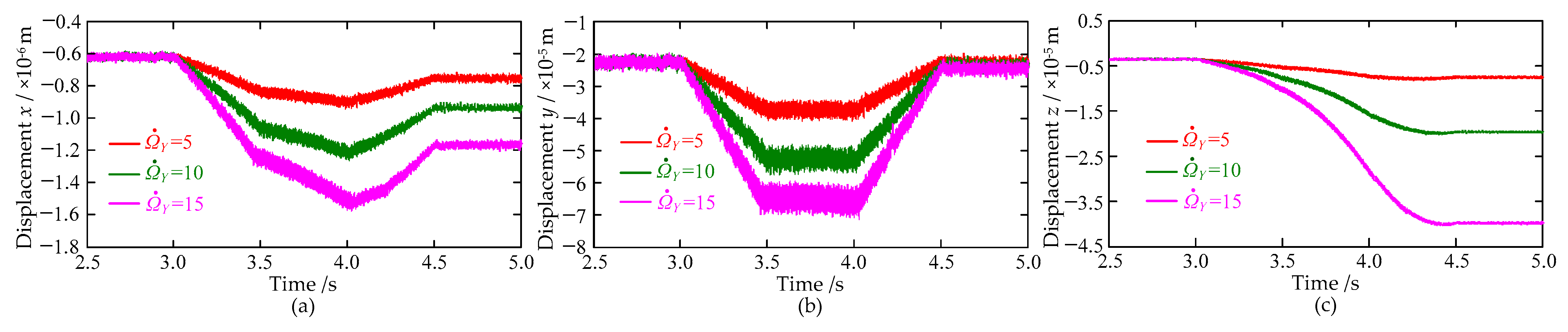
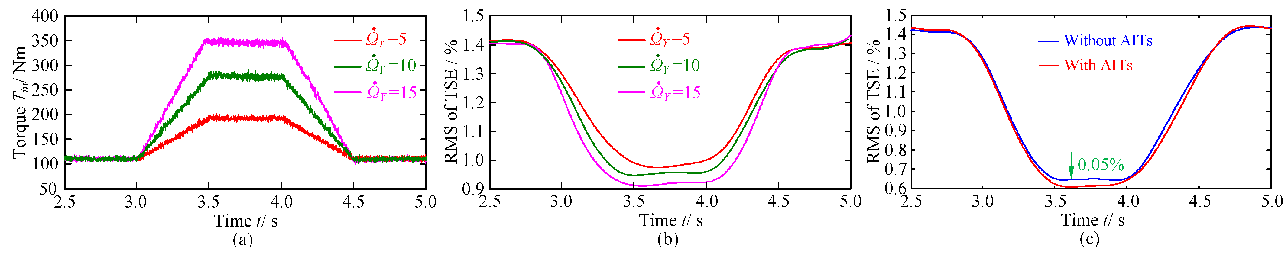
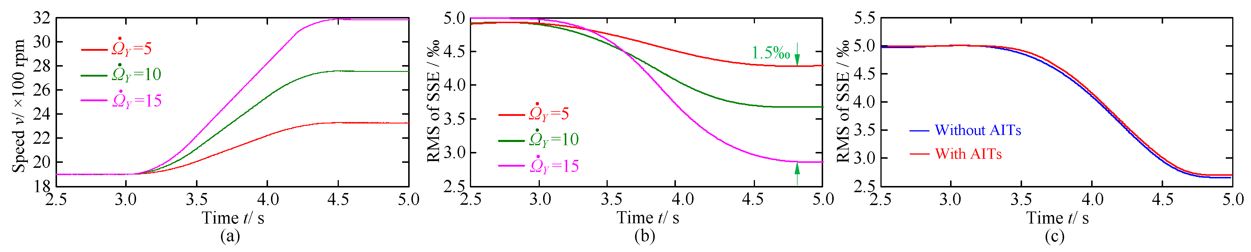
3.2. Case II: The NEVs Perform a Variable Speed Circular Motion

If one supposes that the NEVs perform a variable-speed circular motion with radius R_Ω around the Y-axis, θ_Y is the angle displacement and Ω_Y is the rotating velocity of the vehicle around the Y-axis and they are measured in OXYZ, as shown in Figure 16. The gravity G_j in case II is calculated in the same way as that in case I. For the additional inertial force of node j, F_j = −m_j·(a_jr +a_jc); a_jr and a_jc are the convected acceleration vector and Coriolis acceleration vector of node j, respectively. For the additional gyroscopic moment of node j, M_j = J_j·ω × Ω_Y.

As shown in Figure 17a, the convected acceleration vector a_jr = ${\dot{\mathit{\Omega }}}_Y$ × r_o/j + Ω_Y × (Ω_Y × r_o/j) = ${\dot{\mathit{\Omega }}}_Y$ × (r_j/z + r_j/x + r_j/y) + Ω_Y × (Ω_Y × (r_j/z + r_j/x + r_j/y)) = ${\dot{\mathit{\Omega }}}_Y$ × (r_j/z + r_j/x) + Ω_Y × (Ω_Y × (r_j/z + r_j/x)). One must suppose that a_jr1 = ${\dot{\mathit{\Omega }}}_Y$ × (r_j/z + r_j/x) is the additional first convected acceleration vector and a_jr2 = Ω_Y × (Ω_Y × (r_j/z + r_j/x)) is the additional second convected acceleration vector. Hence, the complex three-dimension spatial problem can be solved in a two-dimensional plane, i.e., the xoz plane. As shown in Figure 17b, (m, n) and (m’, n’) represent the initial position coordinate and instantaneous position coordinate of node j in the xoz plane and x₁o₁z₁ plane, respectively, and the convected acceleration vector a_jr can be derived as

$$\{\begin{array}{l}{\mathit{a}}_{jr1}=\left|{\dot{\mathit{\Omega }}}_Y\times {\mathit{r}}_{o/j}\right|\cdot \cos ({\gamma }_j)\cdot {\mathit{e}}_1-\left|{\dot{\mathit{\Omega }}}_Y\times {\mathit{r}}_{o/j}\right|\cdot \sin ({\gamma }_j)\cdot {\mathit{e}}_3;{\mathit{a}}_{jr2}=-\left|{\mathit{\Omega }}_Y\times ({\mathit{\Omega }}_Y\times {\mathit{r}}_{o/j})\right|\cdot \sin ({\gamma }_j)\cdot {\mathit{e}}_1-\left|{\mathit{\Omega }}_Y\times ({\mathit{\Omega }}_Y\times {\mathit{r}}_{o/j})\right|\cdot \cos ({\gamma }_j)\cdot {\mathit{e}}_3\\ \left|{\dot{\mathit{\Omega }}}_Y\times {\mathit{r}}_{o/j}\right|=\left|{\dot{\mathit{\Omega }}}_Y\right|\cdot \sqrt{{(\mathrm{m}+{\mathrm{m}}^{\prime })}^2+{(\mathrm{n}+{\mathrm{n}}^{\prime })}^2};\left|{\mathit{\Omega }}_Y\times ({\mathit{\Omega }}_Y\times {\mathit{r}}_{o/j})\right|={\left|{\mathit{\Omega }}_Y\right|}^2\cdot \sqrt{{(\mathrm{m}+{\mathrm{m}}^{\prime })}^2+{(\mathrm{n}+{\mathrm{n}}^{\prime })}^2};{\gamma }_j=\arctan ((\mathrm{n}+{\mathrm{n}}^{\prime })/(\mathrm{m}+{\mathrm{m}}^{\prime }))\end{array}$$

(17)

In Figure 17b, v_j is the velocity vector of node j in the xoz plane, and the Coriolis acceleration vector a_jc can be derived as

$$\{\begin{array}{l}{\mathit{v}}_j=v_{jx}\cdot {\mathit{e}}_1+v_{jz}\cdot {\mathit{e}}_3\\ {\mathit{a}}_{jc}=2{\mathit{\Omega }}_Y\times {\mathit{v}}_j=2{\mathit{\Omega }}_Y\times (v_{jx}\cdot {\mathit{e}}_1+v_{jz}\cdot {\mathit{e}}_3)=2{\Omega }_Y\cdot v_{jx}\cdot {\mathit{e}}_2\times {\mathit{e}}_1+2{\Omega }_Y\cdot v_{jz}\cdot {\mathit{e}}_2\times {\mathit{e}}_3=2{\Omega }_Y\cdot v_{jz}\cdot {\mathit{e}}_1-2{\Omega }_Y\cdot v_{jx}\cdot {\mathit{e}}_3\end{array}$$

(18)

where Ω_Y is an angular velocity vector in the y-axis, Ω_Y is an angular velocity of node i around the y-axes and it is a number.

The initial positions and instantaneous positions of nodes i and j are shown in Figure 17c and L_ij represents the initial axial distance between i and j. ($x_i^{\prime }$, $y_i^{\prime }$, $z_i^{\prime }$) and ($x_j^{\prime }$, $y_j^{\prime }$, $z_j^{\prime }$) are the instantaneous position coordinates of nodes i and j. According to the Ref. [23], the additional gyroscopic moment M(t) of any node can be derived as Equation (19), and the terms with a value of zero are not given in Equation (19).

$$\mathbf{M}(\mathrm{t})=-\frac{J\cdot \omega \cdot {\Omega }_Y\cdot [L_{ij}+(z_j^{\prime }-z_i^{\prime })]}{\sqrt{{(x_j^{\prime }-x_i^{\prime })}^2+{(y_j^{\prime }-y_i^{\prime })}^2+{[L_{ij}+(z_j^{\prime }-z_i^{\prime })]}^2}}\cdot {\mathit{e}}_1+\frac{J\cdot \omega \cdot {\Omega }_Y\cdot (x_j^{\prime }-x_i^{\prime })}{\sqrt{{(x_j^{\prime }-x_i^{\prime })}^2+{(y_j^{\prime }-y_i^{\prime })}^2+{[L_{ij}+(z_j^{\prime }-z_i^{\prime })]}^2}}\cdot {\mathit{e}}_3$$

(19)

The ${\dot{\Omega }}_Y$ – t, Ω_Y – t and θ_Y – t curves shown in Figure 18 are used to study the response and synchronizing characteristics of the DMDS when the NEVs perform a variable speed circular motion. Similarly, the initial speed of the vehicle, rotating speeds of PMSMs and load imposed on the DMDS are also 80 km/h, 1900 rpm and 600 Nm, respectively. The turning radius R_Ω is set to 5 m, and the rotating acceleration ${\dot{\Omega }}_Y$ is set to 5, 10 and 15 m·s⁻², respectively. The displacement responses of node 14 (gear node) are shown in Figure 19. The displacement response curves in the y- and z-directions are significantly associated with the ${\dot{\Omega }}_Y$ – t and Ω_Y – t curves, respectively, and the difference is that the directions of the displacement response curves is completely opposite to that of the ${\dot{\Omega }}_Y$ – t and Ω_Y – t curves. However, due to the coupling effect of ${\dot{\Omega }}_Y$ and Ω_Y, the displacement response curves in the x-direction are neither completely related to ${\dot{\Omega }}_Y$ – t nor Ω_Y – t. The displacement responses in three directions increase with the increase in ${\dot{\Omega }}_Y$, but the increases are different.

Based on the above theoretical analysis, under the given non-inertial condition, except for the torque of PMSM (T_in), the nodes are also affected by the following five additional terms: first convected inertial force F_r1, second convected inertial force F_r2, Coriolis inertial force F_c, gyroscopic moment M and gravity G. The displacement responses of node 14 with or without additional inertial terms (AITs) are shown in Figure 20. In the x-direction, after considering AIFs, the displacement increases gradually during the II and III stages, and then decreases during the IV stage, and eventually reaches stabilization during the V stage. The displacement increases from about 0.62 µm to 1.18 µm, an increase of 90.3%, as shown in Figure 20a. In the y-direction, the displacement shows a small increase during the II-V stages, and increases from about 25 µm to 28 µm with an increase of 12% during the V stage. In the z-direction, the difference by not considering AITs is that the displacement increases gradually during the II-IV stages and then tends to become steady during the V stage. Finally, the displacement increases from approximately 3.6 µm to 7.5 µm, with an increase of 108.3%.

Herein, the Equation (14) is also used to calculate the relative influence proportion (γ_i) of the five additional terms and to analyze which terms are the major influence factors and which are the weakest ones, as shown in Figure 21. As demonstrated by the results in Figure 21a, during the I stage, the relative influence proportions of F_r1, F_c and M are greater, reaching 2.9–76%, 9.1–48.6% and 10.6–48.6%, respectively. Then, their relative influence proportions decrease gradually during the II-V stages. However, during the II-V stages, the relative influence proportion of F_r2 starts to increase quickly and becomes the main influence factor, and the maximum proportion can reach 93.9%. In Figure 21b, during the I stage, the relative proportions of G, F_r1, F_c and M are greater, and there is a little difference in their average proportions. Conversely, the relative influence proportion of M tends to become steady after the increase during the II-V stages, the maximum proportion reaches 99.3%, and the relative influence proportions of other additional terms are very small and their influences can be ignored. By comparing Figure 21a,b, it is found that the relative influence proportions of the five additional terms have a similar variation rule, but the shapes of the relative influence proportions of F_c and M in the two figures are exactly opposite. Likewise, the proportions of F_r1, F_c and M are still greater during the I stage and then begin to decrease rapidly during the II-V stages. When it comes to stage II, the proportion of F_r2 begins to increase quickly and then becomes the primary influence factor.

The torque and RMS value of TSE of the PMSMs are shown in Figure 22. Obviously, the curves of torque are very close to the ${\dot{\Omega }}_Y$ – t curve, and increase with the increase in rotating acceleration, as shown in Figure 22a. The results in Figure 22b show that the curves of RMS value of TSE are associated with the ${\dot{\Omega }}_Y$ – t curve, and exhibit a full reversal. Unlike torque, the RMS value of TSE decreases with the increase in rotating acceleration. When ${\dot{\Omega }}_Y$ changes from 5 to 15 m·s⁻², the RMS value of TSE is only reduced from about 1.0% to 0.9%, and the reduction is no more than 10%, indicating that the rotating acceleration also has a small influence on the synchronization of torque between PMSMs. Moreover, the RMS values of TSE with or without AITs are shown in Figure 22c and it can be very clearly observed that the red solid line almost coincides with the blue solid line at all times whether the AITs are considered or not, and the maximum difference does not exceed 0.05%, which means that the influence of AITs on the synchronization of torque between the PMSMs can almost be ignored when the NEVs perform a circular motion.

The speed and RMS value of SSE of the PMSMs are shown in Figure 23. The curves of speed and RMS values of SSE are very close to the ${\Omega }_Y$ – t curve, but the curves of RMS values of SSE and ${\Omega }_Y$ – t have a diametrically opposite changing tendency. The speed increases as the rotating acceleration increases; conversely, the RMS value of SSE decreases as the rotating acceleration increases, with a maximum reduction of no more than 1.5‰, as shown in Figure 23a,b. Combining the results from Figure 23c, it is found that the influence of both AITs and rotating acceleration on the synchronization of speed between PMSMs can also be ignored when the vehicle performs a circular motion.

4. Conclusions

The dynamic model of the DMDS installed on the NEVs was established considering the effects of the non-inertial system in the form of additional inertial terms. The response and synchronizing characteristics of the DMDS under different non-inertial conditions were investigated and compared, and the following conclusions were obtained:

(1) When the NEVs perform a variable speed translational motion, in addition to its own excitation forces and gravity, the components of the DMDS are subjected to an additional convected inertial force caused by the variable speed translational motion. There is a numerically positive correlation between the displacement response of the gears and the translation acceleration, and the contribution of the additional convected inertial force to displacement offset in the x-direction is greater than that of gravity in the y-direction.

(2) Due to the influence of multiple additional inertial terms’ superimposition, the variable speed circular motion of the NEVs results in greater displacement responses. For the displacement responses in the x and z directions, the additional second relative inertial term (namely, the F_r2 term) is the main influence factor among all the additional inertial terms that change the displacement offset. In the y-direction, the additional gyroscopic moment term (namely, the M term) is the dominant influence factor, and its influence is more prominent under high-speed operating conditions.

(3) Regardless of whether the NEVs perform a variable speed translation motion or variable speed circular motion, the acceleration (translation acceleration or rotating acceleration) has a significant influence on the torques and speeds of PMSMs, and they increase with the increase in the acceleration. However, the torque synchronization and speed synchronization between PMSMs is minimally influenced by both the additional inertial terms and the acceleration.

References

1. Yang, H.; Zhang, J.; Wen, X. High Power Dual Motor Drive System Used in Fuel Cell Vehicles. In Proceedings of the IEEE Vehicle Power and Propulsion Conference, Harbin, China, 3–5 September 2008. [Google Scholar]
2. Tang, Y. Dual Motor Drive and Control System for an Electric Vehicle. U.S. Patent 8453770B2, 4 June 2013. [Google Scholar]
3. Inalpolat, M.; Handschuh, M.; Kahraman, A. Influence of indexing errors on dynamic response of spur gear pairs. Mech. Syst. Signal Process. 2015, 60, 391–405. [Google Scholar] [CrossRef]
4. Giagopulos, D.; Salpistis, C.; Natsiavas, S. Effect of non-linearities in the identification and fault detection of gear-pair systems. Int. J. Non-Linear Mech. 2006, 41, 213–230. [Google Scholar] [CrossRef]
5. Setiawan, Y.D.; Roozegar, M.; Zou, T.; Angeles, J. A Mathematical Model of Multi-Speed Transmissions in Electric Vehicles in the Presence of Gear-Shifting. IEEE Trans. Veh. Technol. 2018, 67, 397–408. [Google Scholar] [CrossRef]
6. Sun, W.; Ding, X.; Wei, J.; Wang, X.; Zhang, A. Hierarchical modeling method and dynamic characteristics of cutter head driving system in tunneling boring machine. Tunn. Undergr. Space Technol. 2016, 52, 99–110. [Google Scholar] [CrossRef]
7. Liu, C.; Fang, Z.D.; Liu, X.; Hu, S.Y. Multibody dynamic analysis of a gear transmission system in electric vehicle using hybrid user-defined elements. Proc. Inst. Mech. Eng. Part K J. Multi-Body Dyn. 2018, 233, 30–42. [Google Scholar] [CrossRef]
8. Tang, X.; Hu, X.; Yang, W.; Yu, H. Novel Torsional Vibration Modeling and Assessment of a Power-Split Hybrid Electric Vehicle Equipped with a Dual Mass Flywheel. IEEE Trans. Veh. Technol. 2018, 67, 1990–2000. [Google Scholar] [CrossRef]
9. Zhang, Y.; Spanos, P.D. Efficient response determination of a M-D-O-F gear model subject to combined periodic and stochastic excitations. Int. J. Non-Linear Mech. 2019, 120, 103378. [Google Scholar] [CrossRef]
10. Yan, H.S.; Wu, Y.C. A Novel Design of a Brushless DC Motor Integrated with an Embedded Planetary Gear Train. IEEE/ASME Trans. Mechatron. 2005, 11, 551–557. [Google Scholar] [CrossRef]
11. Mashimo, T.; Urakubo, T.; Shimizu, Y. Micro Geared Ultrasonic Motor. IEEE/ASME Trans. Mechatron. 2018, 23, 781–787. [Google Scholar] [CrossRef]
12. Kim, B.S.; Song, J.B.; Park, J.J. A Serial-Type Dual Actuator Unit With Planetary Gear Train: Basic Design and Applications. IEEE/ASME Trans. Mechatron. 2009, 15, 108–116. [Google Scholar]
13. Lee, H.; Choi, Y. A New Actuator System Using Dual-Motors and a Planetary Gear. IEEE/ASME Trans. Mechatron. 2012, 17, 192–197. [Google Scholar] [CrossRef]
14. Wei, J.; Shu, R.; Qin, D.; Lim, T.C.; Zhang, A.; Meng, F. Study of synchronization characteristics of a multi-source driving transmission system under an impact load. Int. J. Precis. Eng. Manuf. 2016, 17, 1157–1174. [Google Scholar] [CrossRef]
15. Zhao, D.Z.; Li, C.W.; Ren, J. Speed synchronisation of multiple induction motors with adjacent cross-coupling control. Iet Control Theory Appl. 2009, 4, 119–128. [Google Scholar] [CrossRef]
16. Xiong, H.; Zhang, M.; Zhang, R.; Zhu, X.; Yang, L.; Guo, X.; Cai, B. A new synchronous control method for dual motor electric vehicle based on cognitive-inspired and intelligent interaction. Future Gener. Comput. Syst. 2019, 94, 536–548. [Google Scholar] [CrossRef]
17. Shi, T.; Liu, H.; Geng, Q.; Xia, C. Improved Relative Coupling Control Structure for Multi-motor Speed Synchronous Driving System. IET Electr. Power Appl. 2016, 10, 451–457. [Google Scholar]
18. Yang, Y.; Li, M.; Hu, M.; Qin, D. Influence of controllable parameters on load sharing behavior of torque coupling gear set. Mech. Mach. Theory 2018, 121, 286–298. [Google Scholar] [CrossRef]
19. Kahrobaiyan, M.H.; Asghari, M.; Ahmadian, M.T. A Timoshenko beam element based on the modified couple stress theory. Int. J. Mech. Sci. 2014, 79, 75–83. [Google Scholar] [CrossRef]
20. Zhang, A.; Wei, J.; Qin, D.; Hou, S.; Lim, T.C. Coupled Dynamic Characteristics of Wind Turbine Gearbox Driven by Ring Gear Considering Gravity. J. Dyn. Syst. Meas. Control 2018, 140, 1–15. [Google Scholar] [CrossRef]
21. Hu, Z.; Tang, J.; Zhong, J.; Chen, S. Frequency spectrum and vibration analysis of high speed gear-rotor system with tooth root crack considering transmission error excitation. Eng. Fail. Anal. 2016, 60, 405–441. [Google Scholar] [CrossRef]
22. Lu, Z.; Sheng, H.; Hess, H.L.; Buck, K.M. The modeling and simulation of a permanent magnet synchronous motor with Direct Torque Control based on Matlab/Simulink. In Proceedings of the Electric Machines and Drives, San Antonio, TX, USA, 15 May 2005; pp. 1150–1156. [Google Scholar]
23. Zhang, A.; Wei, J.; Shi, L.; Qin, D.; Lim, T.C. Modeling and dynamic response of parallel shaft gear transmission in non-inertial system. Nonlinear Dyn. 2019, 98, 997–1017. [Google Scholar] [CrossRef]
Figure 1. Structure of DMDS.
Machines 10 00620 g001
Figure 2. Dynamic model and node distribution diagram of DMDS.
Machines 10 00620 g002
Figure 3. Equivalent model of meshing element.
Machines 10 00620 g003
Figure 4. Meshing stiffness.
Machines 10 00620 g004
Figure 5. Timoshenko beam.
Machines 10 00620 g005
Figure 6. Equivalent model of connecting elements.
Machines 10 00620 g006
Figure 7. Bearing element.
Machines 10 00620 g007
Figure 8. (a) Kinematic analysis in non-inertial system; (b) analysis of additional gyroscopic moment.
Machines 10 00620 g008
Figure 9. Force analysis diagram: (a) force analysis when NEV travels in a straight line; (b) force analysis of node j.
Machines 10 00620 g009
Figure 10. The curves of translation acceleration ax and translational speed v.
Machines 10 00620 g010
Figure 11. Displacement responses of node 14 under different non-inertial conditions: (a) x-direction; (b) y-direction.
Machines 10 00620 g011
Figure 12. Displacement responses with or without additional inertial forces of node 14 when ax changes from 10 to −10 m·s−2: (a) x-direction; (b) y-direction.
Machines 10 00620 g012
Figure 13. Relative proportion of each influence factor: (a) displacement response in x-direction; (b) displacement response in y-direction.
Machines 10 00620 g013
Figure 14. Torque and TSE when ax changes from 10 to −10 m·s−2: (a) torque of PMSMs; (b) TSE; (c) the changes in RMS of TSE with ax.
Machines 10 00620 g014
Figure 15. Speed and SSE when ax changes from 10 to −10 m·s−2: (a) speed of PMSMs; (b) SSE; (c) the changes in RMS of SSE with ax.
Machines 10 00620 g015
Figure 16. Schematic diagram of circular motion.
Machines 10 00620 g016
Figure 17. Relative motion: (a) displacement vector of node j; (b) convected acceleration vector and Coriolis acceleration vector; (c) rotational angular velocity.
Machines 10 00620 g017
Figure 18. The curves of rotating acceleration Ω ˙ Y , rotating speed ΩY and angle displacement θY in variable-speed circular motion.
Machines 10 00620 g018
Figure 19. Displacement responses of node 14 under different rotating accelerations: (a) x-direction; (b) y-direction; (c) z-direction.
Machines 10 00620 g019
Figure 20. Displacement responses with or without AIF of node 14 when R = 5 m and Ω ˙ Y = 20 m·s−2: (a) x-direction; (b) y-direction; (c) z-direction.
Machines 10 00620 g020
Figure 21. Relative influence proportion of each factor: (a) displacement response in x-direction; (b) displacement response in y-direction; (c) displacement response in z-direction.
Machines 10 00620 g021
Figure 22. Torque and RMS value of TSE: (a) torque of PMSMs under different rotating accelerations; (b) RMS values of TSE under different rotating accelerations; (c) RMS values of TSE with or without AITs.
Machines 10 00620 g022
Figure 23. Speed and RMS value of SSE: (a) speed of PMSM under different rotating accelerations; (b) RMS values of SSE under different rotating accelerations; (c) RMS values of SSE with or without AITs.
Machines 10 00620 g023