Article

GNSS-Free End-of-Row Detection and Headland Maneuvering for Orchard Navigation Using a Depth Camera †

Department of Biological and Agricultural Engineering, University of California, Davis, CA 95616, USA
*
Author to whom correspondence should be addressed.
This paper is an extended version of our paper published in 2022 30th Mediterranean Conference on Control and Automation (MED), Vouliagmeni, Greece, 28 June–1 July 2022.
Machines 2023, 11(1), 84; https://doi.org/10.3390/machines11010084
Submission received: 13 December 2022 / Revised: 6 January 2023 / Accepted: 7 January 2023 / Published: 9 January 2023

Abstract

:
GPS-based navigation in orchards can be unstable because trees may block the GPS signal or introduce multipath errors. Most research on robot navigation without GPS has focused on guidance inside orchard rows; end-of-row detection has not received enough attention. Additionally, navigation between rows relies on reference maps or artificial landmarks. In this work, a novel row-end detection method is presented, which detects drastic changes in the statistical distribution of the sensed point cloud as the robot gets closer to the row’s end. A row-entry method was also implemented that builds a local map that is used by a reactive path tracker. The system was evaluated in a 24-row block in a vineyard. Once the robot was closer than 7 m from the end of a row, the algorithm detected it with a 100% success rate and calculated the distance from it with a mean error of 0.54 m. The system was also evaluated in vineyard configurations with parallel and slanted vine rows in consecutive blocks. The system worked well in all configurations, except where the next block had rows aligned to the rows of the current block and the headland width was closer than 5 m.

1. Introduction

This paper expands upon the work presented in a conference by the authors [1], by adding further related work (Section 2), further details regarding the methodology (Section 3) and the threshold selection process (Section 4.2), and additional experiments to evaluate system performance for different headland configurations (Section 4.3).
Precision agriculture (PA)—the management of spatial and temporal variability in fields using information and communications technologies—can enable significant increases in crop production combined with the sustainable use of agricultural resources. PA was initially developed for annual crops, but its development and adoption have been extended to high-value horticultural production in orchards and vineyards [2]. Agricultural robots can provide advanced sensing, computation, and actuation, enabling PA methods in horticultural production [3]. Autonomous (loosely-supervised) operation is necessary for such robots if orchard operations (e.g., precision spraying, pruning, and harvesting) are to be exercised cost-effectively to address labor shortage challenges.
The ‘building block’ of autonomous operation in orchards is a robust navigation system, which implements three basic tasks: the robot starts at some point in the headland of an orchard block close to a user-defined entrance row (in Figure 1 it is depicted as a green dot); it enters the row (task T1); it travels inside and along the row toward its end (task T2, depicted as an orange arrow in Figure 1); it maneuvers from a position near the end of the row, in the headland, until it gets close to the next row’s entrance (task T3, depicted as a blue arrow in Figure 1); it repeats tasks T1, T2, and T3 to traverse all rows in a desired direction (given by a red arrow in Figure 1) until it traverses the last row of the task (defined by the user) and finishes at a point in the headland (yellow star in Figure 1).
Autonomous field coverage (aka auto-guidance) in open fields relies on cm-level accurate positioning from the RTK-GNSS (Real Time Kinematic Global Navigation Satellite System). In orchards, the implementation of tasks T1, T2, and T3 cannot rely solely on GNSS signals, which are often inaccurate, intermittent, or unavailable due to vegetation-induced multipath or signal blockage. Hence, sensor-based auto-guidance relative to the crop rows is necessary; sensors such as onboard cameras or laser scanners are used to localize the robot relative to the tree rows.

1.1. Detect the End of the Row

Regarding the detection of the end of a row, existing approaches use artificial landmarks [4], features in the data to detect trees and empty space combined with odometry [5], or tree trunk detection and counting along with the assumption that the number of trees in the row is known and that trees are not missed [6]. The main challenge is that near the end of the row, the sensor’s field of view goes beyond the tree line and includes space in the headland and beyond. Depending on the orchard, the ongoing operations, and the location of the block being traversed, this space may be empty or contain moving or stationary objects (e.g., trucks and pump stations), or trees from a neighboring orchard block whose rows are at an angle. All of these possible situations cannot be modeled a priori; therefore, the feature-based detection of row ends is case-dependent and has questionable applicability. Figure 2 shows four common configurations of the headland space at the vineyard block’s exit.
In this paper, we present a method to detect the end of a row and estimate the distance to it—and trigger the transition to T3—which does not rely on features. Instead, our method relies on the observation that near the end of a row, the statistical distribution of the points sensed by a 3D sensor changes drastically compared to the points inside the row. To detect the change, we combine two methods. First, a recent method is used to estimate the robot’s pose relative to the row centerline [7]. This method does not rely on features and provides an estimate of the pose uncertainty that increases significantly as the robot gets closer to the row end (because fewer points belong to the trees of the row). The histogram of the sensed point cloud is used to reject perceived points with a low probability of belonging to trees inside the row. The performance of the row-end detection method was evaluated in configurations with vine rows on the other side of the headland (Figure 2). Such rows contribute points to the sensed point cloud and can negatively influence the algorithm.

1.2. Maneuver to the Next Row

The major existing approaches to implement task T3 rely on a reference map, artificial landmarks or tree detection, and odometry [8]. However, artificial landmarks are costly to install and maintain; pose estimation that relies solely on odometry results in drift errors during headland maneuvering, which may lead to collisions with trees or orchard infrastructure (e.g., trellis posts). Hence, robust headland maneuvering is required to drive the robot into the next row safely. In this work, a local map of the surroundings is updated in real time based on recent point cloud measurements, and a reactive path planner guides the robot into the next row. The proposed methods for end-row detection and maneuvering to the next row were implemented as components of a complete orchard navigation system, which was evaluated on a campus vineyard using a custom-built robot.
In summary, the main contributions of this paper are a method to detect the end of a row and estimate the distance to it, which does not rely on features, and the evaluation of the method in vineyard configurations I and II, which contribute points to the sensed point cloud and can negatively influence the algorithm.
The paper is organized as follows. We first give an overview of related work in Section 2. The applied methodology and materials are presented in Section 3. The field experiments and the relevant results are presented in Section 4. Finally, Section 5 gives a conclusion and outlook for future research.

2. Related Work

Most research in crop-relative navigation has focused on row traversal (T2). Various approaches for navigation in orchards have been pursued that do not utilize GNSS during T2. These approaches usually use onboard sensors, such as 2D/3D light detection and ranging (Lidar) sensors, or a monocular or stereo camera to detect navigation/localization references such as tree trunks, canopies, row centerline, or free space in the robot frame, and use them for relative guidance. Chebrolu et al. [9] proposed a localization system that fused data from an onboard monocular camera and an odometer and used a reference map. Bergeman et al. [8] presented a perception and navigation system that used a 2D laser scanner and wheel and steering encoders. A similar approach was proposed for linear crops by Ahmadi et al. [10]. They used a visual-servoing-based controller that relied on local directional features extracted from images captured by a camera that viewed the crop and robot from above. This method is not applicable in most orchards because tree canopies would occlude the camera’s view. Sharifi et al. [3] proposed a vision-based row guidance approach. They used a monocular camera to capture red–green–blue (RGB) images and applied computer vision techniques to extract lines at the ground level defined by the tree rows, and used them as navigation reference. Their method does not utilize deep learning and relies on traditional feature extraction. Cerrato et al. [11] utilized deep learning techniques and synthetic data generation to train a segmentation network to segment crops/foliage in RGB images. They also designed a segment-based control algorithm to steer the robot inside the row by keeping it in the row center. Their method was developed in simulation and was evaluated in actual vineyards and pear orchards.
Some researchers have investigated the headland maneuvering and row-switching task (T3). Bergeman et al. [8] placed artificial landmarks (reflective tape) at both ends of each row in an apple orchard and used a laser scanner to detect them and localize the robot with respect to them. Marden et al. [12] developed a line-based simultaneous localization and mapping system (SLAM) with a 2D Lidar. When the robot travels inside a row, it keeps planning a U-turn path to enter the next row and checking the interference of the path with the mapped surrounding environment. The U-turn path will be executed when it does not interfere with mapped obstacles. However, this work is sensitive to gaps in the tree rows (e.g., missing trees and orchard alleys) and does not compensate for drift errors during headland turning. Adrien et al. [13] designed a sensor-based controller for U-turn navigation in orchards. They used a laser range finder sensor to find the distance and angle from the end of the row (last tree trunk). They proposed two sensor-based control laws to enable the robot/vehicle to turn following particular spirals around the end of the row. Their method was a significant improvement over methods that relied on dead reckoning; however, this method relies on clearly detecting the last tree trunk, which can be challenging in some scenarios where tree trunks are not visible (Figure 3). Furthermore, their method was only tested in a simulated environment. Emmi et al. [14] proposed the notion of a hybrid topological map that benefits from general partitioning of the row–crop field and contains well-separated (disjointed) workspaces. The key locations and working areas are identified using onboard sensors (RGB camera, 2D Lidar), and the robot’s pose (state) in the field is probabilistically estimated. They evaluated their approach using only offline data.
Robust ways to sense the end of the row during T2 (to trigger a transition to T3), and implement T3, have not received enough attention. The work proposed in this paper differs from the previous approaches in that it uses a novel row-end detection method to detect drastic changes in the statistical distribution of the sensed point cloud as the robot gets closer to the row end, along with a row-entry method that uses a reactive path tracker with online local map building. The combined system allows the mobile robot to (i) autonomously navigate through vineyard rows without any GNSS solutions, and artificial landmarks, (ii) detect the row ends and row entries in row-to-row traversing, and (iii) maneuver row-end turning to the new row in the headland space. This system has been verified in an actual vineyard.

3. Materials and Methods

3.1. Background: In-Row with Template-Based Localization

The in-row template-based localization method [7] constructs a 3D “sensing template” T, which is a 3D grid that contains voxel occupancy frequency in the camera’s field of view (FOV). The template is constructed during the initial training phase and represents what a 3D camera expects to measure when placed on the centerline of a typical orchard row. After training, Monte Carlo localization [15] is used to compute the robot’s pose when the robot navigates inside rows, which results in the optimal alignment between the sensed point cloud and the template T.
The outputs of template localization are expressed in the frames shown in Figure 4. {R} is the currently traversed orchard row frame. Its origin is on the centerline of the row, between the first pair of trees at the row entrance. Its X-axis is the centerline of the row and points forward to the other end of the row, and its Z-axis points upward. {V} is the vehicle frame, with its X-axis pointing forward and the Z-axis pointing upward. The point cloud is in the camera frame {C}. The rigid-body transformation between {C} and {V} is known and fixed. The row template frame {T} has the same orientation as {R}, and its origin lies on the centerline and at the same x-coordinate as {V} with respect to {R}.
At each time step, the template localization algorithm outputs: (a) the robot pose relative to the centerline, y ,   θ T , where y represents the lateral displacement, and θ represents the heading relative to the centerline; (b) a covariance matrix for y and θ . The uncertainties in y ( σ y ) and θ ( σ θ ) increase as the robot approaches the end of the row; the deviation σ θ is less noisy, hence it is used for row-end detection in this work. As the robot gets closer to the end of the row, fewer and fewer trees in front of it align in two rows and the point cloud distribution deviates more from the template. This manifests itself in an increasing σ θ that is used to robustly estimate the distance to the row’s end, despite missing trees and canopy irregularities.

3.2. State Machine of Orchard Navigation

The navigation task is modeled by a finite state machine (FSM), shown in Figure 5 (left). An example of the state transitions during navigation is illustrated in Figure 5 (right).
In the “START” state of the FSM, the robot is in the headland, close to the first row to be traversed and aligned with it. In this state, the robot keeps moving forward and checking if the “Row Entry Detected” condition is satisfied. The “Row Entry Detected” becomes true if σ θ is less than a threshold, σ θ t h r e s h o l d , and the number of valid measurements, N v a l i d , is consistently higher than a threshold, N v a l i d t h r e s h o l d in the previous five frames (to eliminate chattering). The “valid measurements” are defined as the sensed 3D points whose corresponding template voxels have an occupancy probability greater than a threshold [7]. The selection of σ θ t h r e s h o l d and N v a l i d t h r e s h o l d is discussed in the experiments section.
In the “IN_ROW_NAVIGATE” state, the robot navigates using the in-row template localization method. The reference waypoints are generated on the row’s centerline, starting from the origin of {T} (blue dots in Figure 6). The waypoints are transformed into the vehicle frame {V} and tracked by the robot with a pure-pursuit controller. The robot transitions to the state of “U_TURN_NAVIGATE” when the condition of “Row End Detection” becomes true; otherwise, it keeps moving along the row centerline. The criterion is evaluated by checking if the estimated distances to the row’s end are consistently smaller than a threshold, d e , in the previous five frames (to eliminate chattering). The estimation of the row-end distance is introduced in Section C, while the selection of d e is discussed in the experiments section. At the instant when “Row End Detection” is satisfied, the endpoint of the row is estimated in {T}, as described in Section C.
In the “U_TURN_NAVIGATE” state, waypoints are generated using the estimated endpoint of the row and the designated row traversal direction (Figure 6). The waypoints are generated initially in the {T} frame and transformed into the vehicle frame {V} given ( y , θ ) T at that instant. Then, the U-turn waypoints are transformed into the vehicle frame {V} using the frame-to-frame transformation estimated with odometry. In this state, a reactive path tracker is used to maneuver the robot to the next row despite localization and control errors (described in Section D). The robot returns to the “IN ROW NAVIGATE” again once “Row Entry Detected” becomes true.

3.3. Detection of the End of the Row

Near the end of the row, the number of points that belong to the trees on the left and right of the robot gradually reduces. Given y ,   θ T , we transform the point cloud of tree rows from {V} to template frame {T}. In {T}, the ground plane is obtained with the random sample consensus (RANSAC) algorithm [7]. The measured 3D points from the ground to the top of the plant (Z-axis of {T}) are assumed to be 3D points of tree rows. The points are separated into left and right tree rows using the detected row centerline. One-dimensional histograms of x-coordinates of the left and right tree row points are then computed with equal-width ( δ r ) bins from the origin of {T} to the measured range, d f , of the depth camera (Figure 7).
When the frequency of 3D points on the turning side is smaller than a percentile threshold ( P t h r e s h ), the corresponding segments are labeled as sparse-point segments. P t h r e s h is computed from the frequency histograms of the x-coordinates of the left and right (tree canopy) points in {T}, when the robot is near the end of the row. Namely, the mean, μ, and standard deviation, σ, of all bins are calculated, and the threshold P t h r e s h is set equal to μ-2σ.
When the template localization has high certainty (low σ θ and high N v a l i d ), the farthest sparse-point segment from the robot is regarded as the row-end segment. While the template localization is uncertain, or the estimated distance to the row end is greater than d f , the estimated distance in the X-axis is set to d f . The estimation of the distance to the end of the row is depicted in pseudocode in Algorithm 1, where X T represents the x-coordinates of the left ( X L T ) or right ( X R T ) tree row points in {T}. When the “Row End Detected” condition is satisfied, the row endpoints are estimated in {T}. The x-coordinate of the row end in {T} is the estimated distance to the row end, x e n d T , and the y-coordinate is determined based on the available row width.
Algorithm 1: Row-end distance estimation
Inputs: d f , δ r , X T ,     σ θ t h r e s h o l d , and N v a l i d t h r e s h o l d
Output: x e n d T
H , X e d g e s = Histogram1D ( X T ,   d f , δ r )
for i = N b : 1 do:
if H[i] < P t h r e s h   :
  break
if   σ θ < σ θ t h r e s h o l d   a n d   N v a l i d > N v a l i d t h r e s h o l d   :
x e n d T = m i n ( X e d g e s i , d f )  
else:
   x e n d T   =   d f

3.4. Maneuver to the Next Row

A reactive approach was adopted to compensate for localization and control errors during turning. A dynamic 2D local occupancy grid map is generated from the point cloud. A reactive path planner generates suitable waypoints to exit the current row, turn, and then enter the next row [16].
In this work, only one depth camera on the front side of the mobile robot was used. The robot’s perception capability is enhanced with a local mapping technique. The applied algorithms achieve two targets: (1) filter out the noisy data from the depth camera, and (2) expand the camera’s FOV to execute a U-turn in the headland space. The local map range has width w and length ( d f + d m ) relative to the origin of {V}, as shown in Figure 8. d m is the approximate distance the robot traverses in duration D, given the running speed of the robot. The measuring range of the depth camera projected on the 2D plane is simplified as a sector area determined by the camera’s FOV.
The local map is updated as an occupancy grid [17]. First, the 3D points over the ground plane (found with RANSAC) are projected onto a 2D grid map. A 2D array H p is used to represent the probabilities of each occupied cell. Second, the cached frames are split into N earlier and N later frames. The earlier N frames cover the area behind the robot, and the later frames cover the area ahead of the robot. The projected points in earlier frames are first used to calculate the cell probabilities in the mapping range. The cell probabilities in the grid map are calculated using Equation (1). In each frame, a cell is considered occupied when its center is in the measuring range (sector area) of that frame and there is at least one projected point. Then, the cell probabilities covered by points in late frames are calculated similarly. The cell probabilities from late frames overwrite the overlapping cell probabilities.
P ( o c c u p i e d | m e a s u r e d ) = N u m b e r   o f   c e l l s   o c c u p i e d   &   m e a s u r e d   N u m b e r   o f   c e l l s   m e a s u r e d
This approach makes the robot more responsive to the tree rows and infrastructure obstacles observed in late frames and maintains a large FOV during U-turns. A G a u s s i a n B l u r function is applied to the calculated array H p to filter out noise in the data. If the grid probability in H p is larger than a threshold, the value in H p is labeled as 1; otherwise, it is labeled as 0. Finally, the occupied cells are combined, and the regions they cover are modeled as polygons representing obstacles in the robot’s environment.
The robot navigation subtask is to follow the planned waypoints without colliding with the detected obstacles. The motion control of the robot is similar to the scheme of active localization [18]. A dynamic window path planner reactively generates a collision-free path near the reference waypoints. This way, the robot can enter the new row robustly and safely. Figure 9 shows an example of when the robot has just entered a row: the robot exited the top row moving to the left, and entered the second row from the top, moving to the right). The waypoints (cyan dots) of the reference path were computed by the robot at the instant when the “Row End Detected” condition became true and contained orientation drift error relative to the new row centerline as the robot maneuvered the U-turn in the headland. The reactive path planner guides the robot toward the middle of the new row (curved path segment in red color), away from the obstacles (plant rows), and enables a safe transition to the “IN_ROW_NAVIGATE” state.

3.5. Row Entry Detection

The guided path leads the robot to the next row through a U-turn maneuver (T3). After the U-turn starts, the robot switches back to the “IN_ROW_NAVIGATE” state after the template localization is obtained with high certainty (low σ θ and high N v a l i d ) and the heading change is greater than a threshold. The heading difference is around 180 degrees for a typical U-turn maneuver between rows. Considering the drifting issues of localization from wheel odometry, the threshold is set at a value lower than 180 degrees and larger than 90 degrees.

3.6. Experimental Setup

The navigation system was tested on a mobile robot in a vineyard on the UC Davis campus. GNSS signals were available and used only for ground truth. The software of the robot system was built upon ROS (Robot Operating System). The localization module was programmed with C++, and the path planning and tracking modules were programmed using Python programming language.
A custom-built mobile robot (Figure 10) was used in the experiments. A computer (NUC, Intel®) with a Core i3 processor performed all of the computation. A depth camera (D435, Intel® RealSense™) was installed at the front of the robot (range df = 12 m), and two RTK-GPS receivers (Piksi® Multi, Swift Navigation) were used to obtain the position and heading of the robot in the geodetic frame. The control update rate—including localization and row-end detection—was 8 Hz. The experiments took place in a campus vineyard, and the small height of the canopies made it possible to use the RTK-GPS to record ground truth pose. The length of each row was approximately 25 m, and the row spacing was 3.6 m. A map of twenty-five rows was built from a satellite map of the vineyard. The map consisted of two endpoints for each row (yellow points and respective lines in Figure 11). The top and bottom (in Figure 10) headland spaces correspond to configurations III and IV, respectively.
Initially, the robot traversed the first four rows of the vineyard following a reference path and localizing itself on the map based solely on the GNSS solution. The goal was to collect data for the selection of the thresholds σ θ t h r e s h o l d , and N v a l i d t h r e s h o l d , as explained in Section 3.2. After threshold selection, the following navigation task was executed: start at an initial row (row 1), traverse 24 rows to the left at the speed of 0.8 m/s, and stop at the end of the 24th row (Figure 9). The robot executed the task using the 3D camera and odometry data (GNSS was used only as ground truth).
As mentioned above, the vineyard’s headlands corresponded to configurations III and IV. To assess the performance of the row-detection algorithm in headland configurations I and II, these configurations were simulated using sensor data gathered during our experiments, as explained in Section 3.4.

4. Experiments and Results

4.1. Threshold Selection

The uncertainty of the template-based localization depends on the number of points measured by the depth camera from the tree rows [7]. As the robot approaches the end of the row, fewer trees remain inside the camera’s FOV. The estimated heading deviation, the number of valid measurements, and the distance to the end of the row are shown in Figure 12, plotted as a function of the robot’s distance to the row end (which ranges from 20 m to 0 m). Figure 11a shows that while the robot is farther than 7.5 m from the end of the row, the heading deviation is small, with a mean value of 0.06 rads, and exhibits small fluctuation about the mean. The mean heading deviation and its fluctuation increase between 7.5 and 5 m away from the row end and increase drastically after the camera is less than approximately 4 m away from the row end. The selected threshold value for the heading uncertainty was set to three times the mean value of the heading deviation, i.e., σ θ t h r e s h o l d = 0.18 , a value that was expected to be exceeded at roughly 5 m from the row end.
Figure 11b shows that while the robot is farther than about 9 m from the end of the row, the average number of valid points is approximately constant, with a small fluctuation of about a mean of 1400 points. The number of valid points decreases until the robot is about 5 m from the row end and then decreases dramatically between 5 and 2.5 m from the row end (the specific numbers will depend on the FOV of the depth camera). The number increases when the camera gets closer to the goal because points from beyond the headland are sensed. The threshold for the number of valid points was set to N v a l i d t h r e s h o l d = 1000 to ensure that enough points are present and that distances larger than 5 m are considered “far” from the row end, as per the selected value for σ θ t h r e s h o l d .
The distance to the end of the row is estimated in the state of “IN ROW NAVIGATE.” This distance cannot be longer than df (12 m) (Algorithm 1). Hence, the estimated errors are biased for this specific measuring range when the robot is over 12 m from the row end. As shown in Figure 11c, as the camera approaches the end of the row, the biased error of the estimated distance to the end of the row becomes smaller. It reaches a minimum value near 7 m from the row’s end and increases again as fewer trees are in the camera’s FOV. The row-end distance threshold ( d e ) is set to 7 m, where the row-end detection error was small. It is important to note that at distances farther than d e , the thresholds for the heading deviation and the number of valid measurements are not exceeded, so the template results can be used in Algorithm 1.
For the row-entry detection, the same thresholds as above are applied to check if the template localization has high certainty. Considering the drift errors for the orientation estimation from wheel odometry, the threshold was set at 120 degrees.

4.2. Experiments to Evaluate System Performance

Figure 13 depicts the robot’s path as it traversed the first 10 rows during the experiments (more rows are not shown due to page limit constraints). The red dashed line depicts the desired path, which was generated considering the robot’s turning radius and the field’s map (straight yellow lines). The solid line represents the actual path of the robot with the proposed methodology. The blue segments represent the robot path in the “IN_ROW_NAVIGATE” state. The red segments correspond to the robot path in the “U_TURN NAVIGATE” state.
The red dots corresponded to the locations when the “Row Entry Detected” condition was triggered. The green stars correspond to positions where the robot detected the row end and entered the “U_TURN NAVIGATE” state. The yellow diamonds correspond to the detected row ends transformed in the geodetic frame at the instant when the “Row End Detected” condition was triggered. The row-end positions obtained from satellite images were used as ground truth positions. The row ends were detected with a 100% success rate. The mean of the distance error was 0.54 m, and its standard deviation was 0.45 m.
The thresholding methods used to trigger the transitions between the “IN ROW NAVIGATE” and “U_TURN NAVIGATE” states are visualized in Figure 14a–c. The blue points represent navigation in the headlands, and the red points represent the navigation inside the vineyard rows. The red dashed lines in Figure 14a–c represent the applied thresholds. The blue line in Figure 14d shows transitions during the experiment between the “IN ROW NAVIGATE” (‘1’) and “U_TURN NAVIGATE” (‘0’) states.
According to the FSM, the robot should enter “U_TURN NAVIGATE” at de where the in-row template localization fails and enters “IN ROW NAVIGATE” after aligning with the first tree in the next row. In this ideal situation, we assume that the robot transitions to “U_TURN NAVIGATE” at d e x e n d T = 7   m away from the row end and transitions to “IN ROW NAVIGATE” when it is aligned with the first tree of the new row. The robot state in this ideal situation is plotted in Figure 14d as a red dashed line. One can see that the applied state transitions work very well. The in-row navigation typically starts a little earlier before the robot enters the new row, as the row entry can be found before entering.
Figure 15 shows the heading deviation, the valid point ratio (the number of valid points divided by 1000), and heading changes while the robot did the U-turn maneuver. The robot’s heading in the figure was measured directly from the GNSS system.

4.3. Algorithm Performance for Different Headland Configurations

As mentioned above, the estimation of the row’s endpoint starts when the robot is 7 m away from the end of the row. Therefore, headlands wider than 7 m cannot affect the algorithm’s performance. However, the row-end detection algorithm may be affected when the distance of the current block to the next block (headland width) is smaller than 7 m. Among the four typical headland space configurations presented in Figure 2, the most challenging ones are configurations I and II, in which the rows between neighboring blocks are parallel and aligned or slanted to each other. (In configurations III and IV, the point clouds at the row exit are very different from the ones inside the row.) We used the data collected in the experiments from the depth camera and GNSS to simulate the point cloud that the sensor would record in configurations I and II and to evaluate the row-end detection algorithm’s performance. Essentially, simulated tree rows with different positions and orientations were ‘stitched’ at the end of the block to create configurations I and II and generate corresponding point clouds. The simulated row-ending conditions are shown in Figure 16. The row gap was set at 4 m in Figure 16b.
In the simulation, the robot moved along the centerline of the row (red dashed line) toward the left (+X direction), as shown in Figure 16. The small black arrows around the red line correspond to the localization results from the template localization algorithm. The template localization performed well in both configurations before reaching the green line (7 m from the row end). In Figure 14a, the localization results (deviation from the centerline) were consistently worse after the green line. However, in Figure 16b the deviation increases for a while and then becomes very small again as the robot gets closer to the next block (the one on the left). The reason is that the points from the rows of the next block align very well with the point cloud perceived in the row currently being traversed. Drastic changes in both the valid points ratio and the estimated deviation of the yaw angle trigger the state transition from T1 to T2.
These two metrics were evaluated and plotted in Figure 17, which shows the valid points ratio (valid points count/1000) as blue dotted curves and the estimated deviation of the yaw angle (orange dotted curves) as functions of the x-coordinate of the robot. Figure 17a shows that when the next vineyard block contained slanted rows, there were drastic changes in both the valid points ratio and the heading deviation as the robot approached the end of the row, even when the headland was narrow (4 m). The reason for this is that random points from the neighboring rows (orange points in Figure 16) entered the FOV of the Lidar, and many of them did not match/align with the sensor template of the current block rows. Therefore, the number of valid points and the deviation of the estimated heading output by the template-matching algorithm fluctuated a lot; the row-end detection algorithm could detect the end of the row and trigger the transition to a U-turn. In contrast, Figure 17b shows that when the neighboring block rows were parallel and aligned, the headland width was small (here, 4 m), and the valid points ratio and the deviation of the estimated yaw angle did not change significantly as the robot moved closer to the end of the row because the points from the neighboring block matched those of the row template. This result indicates that the algorithm will fail in type I configurations.
To further evaluate the effect of headland width on these metrics (valid points and yaw estimation deviation), two more simulated experiments were performed with different headland distances at 5 m and 6 m. The results are shown in Figure 18. Overall, the points from the neighboring block rows inside the Lidar’s FOV align well with the sensor template of the current block. When the distance was 6 m, there was enough of a gap in the data (there were no points in the headland) for the template-matching algorithm to detect the end of the row. However, when the headland width was 5 m (narrower), the deviation metrics did not change drastically, and the template-matching algorithm was “fooled” into thinking that all points belonged to rows in one block.

5. Discussion

This paper presents a navigation system for a mobile robot that traverses orchard rows using a 3D camera and odometry data and does not rely on GNSS and artificial landmarks. The system estimates the robot’s distance from the end of the tree rows and executes a U-turn to the next row. The row-end detection algorithm detects drastic changes in the statistical distribution of the point cloud sensed by the camera. The system constructs a local map, and a reactive path tracker drives the robot into the next row.
The navigation method was evaluated using a mobile robot that was tasked to traverse 24 rows in a vineyard block. The evaluation results showed that once the robot was closer than 7 m from the end of the row, the proposed row-end estimation method always detected the row end and calculated the distance from it with a mean error of 0.54 m. The performance of the row-end detection method was also evaluated in configurations where there were vine rows on the other side of the headland of the currently traversed block. Such rows contribute points to the sensed point cloud and can negatively influence the algorithm. Row-end detection and distance estimation worked well in all configurations except when the next block had vine rows aligned and parallel to the rows of the current block and the headland width was closer than 5 m (too close).
There are several ways to improve the proposed approach. First, a simultaneous localization and mapping (SLAM) algorithm can be combined with the FSM to achieve global localization. Second, the thresholds could be automatically computed from the sampling rows by utilizing statistical testing algorithms. Finally, appropriate points cloud features could be extracted and used to detect end-of-row instances when neighboring blocks are close together and have aligned tree rows.

Author Contributions

Conceptualization, C.P., Z.F. and S.G.V.; software, C.P. and Z.F.; formal analysis, C.P., Z.F. and S.G.V.; writing—original draft preparation, C.P.; writing—review and editing, C.P., Z.F. and S.G.V.; project administration, S.G.V.; funding acquisition, S.G.V. All authors have read and agreed to the published version of the manuscript.

Funding

This research was funded by USDA-NIFA grant 2020-67021-30759 and USDA-NIFA AFRI Competitive Grant no. 2020-67021-32855/project accession no. 1024262, administered through AIFS: the AI Institute for Next Generation Food Systems.

Data Availability Statement

The data presented in this study are available on request from the corresponding author.

Conflicts of Interest

The authors declare no conflict of interest.

References

  1. Peng, C.; Fei, Z.; Vougioukas, S.G. Depth camera based row-end detection and headland maneuvering in orchard navigation without GNSS. In Proceedings of the 2022 30th Mediterranean Conference on Control and Automation (MED), Vouliagmeni, Greece, 28 June–1 July 2022; pp. 538–544. [Google Scholar] [CrossRef]
  2. Zude-Sasse, M.; Fountas, S.; Gemtos, T.A.; Abu-Khalaf, N. Applications of precision agriculture in horticultural crops. Eur. J. Hortic. Sci. 2016, 81, 78–90. [Google Scholar] [CrossRef]
  3. Sharifi, M.; Chen, X. A novel vision-based row guidance approach for navigation of agricultural mobile robots in orchards. In Proceedings of the 2015 6th International Conference on Automation, Robotics and Applications (ICARA), Queenstown, New Zealand, 17–19 February 2015; pp. 251–255. [Google Scholar] [CrossRef]
  4. Vougioukas, S.G. Agricultural Robotics. Annu. Rev. Control. Robot. Auton. Syst. 2019, 2, 365–392. [Google Scholar] [CrossRef]
  5. Subramanian, V.; Burks, T.F. Autonomous vehicle turning in the headlands of citrus groves. In Proceedings of the 2007 ASAE Annual Meeting, Nashville, TN, USA, 9–12 August 2007; American Society of Agricultural and Biological Engineers: St. Joseph, MI, USA, 2007. [Google Scholar] [CrossRef]
  6. Shalal, N.; Low, T.; McCarthy, C.; Hancock, N. Orchard mapping and mobile robot localisation using onboard camera and laser scanner data fusion—Part B: Mapping and localisation. Comput. Electron. Agric. 2015, 119, 267–278. [Google Scholar] [CrossRef]
  7. Fei, Z.; Vougioukas, S. Row-sensing templates: A generic 3D sensor-based approach to robot localization with respect to orchard row centerlines. J. Field Robot. 2022, 39, 712–738. [Google Scholar] [CrossRef]
  8. Bergerman, M.; Maeta, S.M.; Zhang, J.; Freitas, G.M.; Hamner, B.; Singh, S.; Kantor, G. Robot farmers: Autonomous orchard vehicles help tree fruit production. IEEE Robot. Autom. Mag. 2015, 22, 54–63. [Google Scholar] [CrossRef]
  9. Chebrolu, N.; Lottes, P.; Läbe, T.; Stachniss, C. Robot localization based on aerial images for precision agriculture tasks in crop fields. In Proceedings of the 2019 International Conference on Robotics and Automation (ICRA), Montreal, QC, Canada, 20–24 May 2019; pp. 1787–1793. [Google Scholar] [CrossRef]
  10. Ahmadi, A.; Nardi, L.; Chebrolu, N.; Stachniss, C. Visual servoing-based navigation for monitoring row-crop fields. In Proceedings of the 2020 IEEE International Conference on Robotics and Automation (ICRA), Paris, France, 31 May 2020–31 August 2020; pp. 4920–4926. [Google Scholar] [CrossRef]
  11. Cerrato, S.; Mazzia, V.; Salvetti, F.; Chiaberge, M. A deep learning driven algorithmic pipeline for autonomous navigation in row-based crops. arXiv 2021, arXiv:2112.03816. [Google Scholar]
  12. Marden, S.; Whitty, M. Gps-free localisation and navigation of an unmanned ground vehicle for yield forecasting in a vineyard. Recent Advances in Agricultural Robotics. In Proceedings of the International Workshop Collocated with the 13th International Conference on Intelligent Autonomous Systems (IAS-13), Padova, Italy, 15–18 July 2014. [Google Scholar]
  13. Durand-Petiteville, A.; Le Flecher, E.; Cadenat, V.; Sentenac, T.; Vougioukas, S. Design of a sensor-based controller performing u-turn to navigate in orchards. In Proceedings of the 14th International Conference on Informatics in Control, Automation and Robotics, Madrid, Spain, 26–28 July 2017; SciTePress: Madrid, Spain, 2017; Volume 2, pp. 172–181. [Google Scholar] [CrossRef]
  14. Emmi, L.; Le Flécher, E.; Cadenat, V.; Devy, M. A hybrid representation of the environment to improve autonomous navigation of mobile robots in agriculture. Precis. Agric. 2021, 22, 524–549. [Google Scholar] [CrossRef]
  15. Thrun, S.; Burgard, W.; Fox, D. Probabilistic robotics. Kybernetes 2006, 35, 250. [Google Scholar] [CrossRef]
  16. Nethery, J.F.; Spong, M.W. Robotica: A mathematica package for robot analysis. IEEE Robot. Autom. Mag. 1994, 1, 13–20. [Google Scholar] [CrossRef] [Green Version]
  17. Thrun, S. Probabilistic algorithms in robotics. Ai Mag. 2000, 21, 93. [Google Scholar]
  18. Stachniss, C.; Hahnel, D.; Burgard, W. Exploration with active loop-closing for FastSLAM. In Proceedings of the 2004 IEEE/RSJ International Conference on Intelligent Robots and Systems (IROS), Sendai, Japan, 28 September–2 October 2004; IEEE Cat. No. 04CH37566. Volume 2, pp. 1505–1510. [Google Scholar] [CrossRef]
Figure 1. Top view (from a satellite image) of a typical vineyard block: vines, rows between the vines, and headland space. The symbols represent a typical field coverage navigation task. The robot starts at an initial position near the entrance of a user-defined row (green dot); it traverses a set of rows (orange vertical arrows) toward a specific direction (red arrow points from left to right); and exits from a user-defined row (yellow star).
Machines 11 00084 g001
Figure 2. Four common cases of the headland space at the exit from a vineyard block. (a) Configuration I: the rows between adjacent blocks are parallel; (b) configuration II: the rows between adjacent blocks are slightly slanted; (c) configuration III: the rows between adjacent blocks are almost perpendicular; and (d) configuration IV: there is no adjacent block.
Machines 11 00084 g002
Figure 3. Tree trunks are blocked by tall grass.
Machines 11 00084 g003
Figure 4. The figure shows the orchard row frame {R}, the vehicle frame {V}, the template frame {T}, and the definition of lateral and heading offsets.
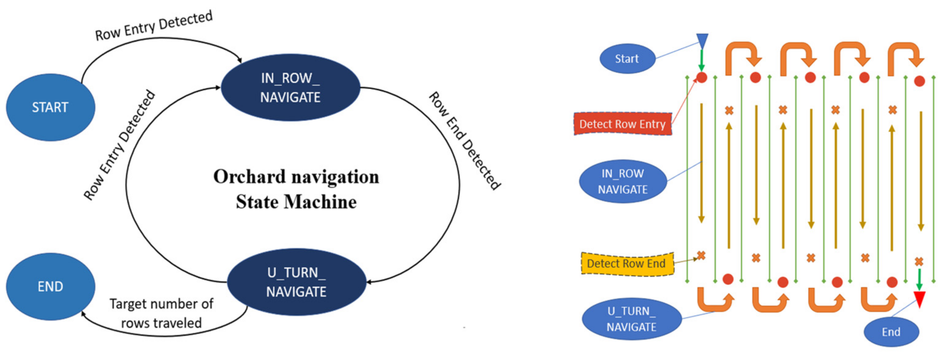
Machines 11 00084 g004
Figure 5. State machine model for orchard navigation (left); robot states illustrated on a skeleton field map (right).
Machines 11 00084 g005
Figure 6. Waypoints generated in different states. The blue points are generated in the “IN_ROW _NAVIGATE” state. The red points are generated in the “U_TURN_NAVIGATE” state.
Machines 11 00084 g006
Figure 7. Frequency histograms of the x-coordinates of the left and right (tree canopy) points in {T} when the robot is near the end of the row. The red bins represent the detected row-end segment. The stars are the manually measured row endpoints. The blue dashed line is the detected row centerline.
Machines 11 00084 g007
Figure 8. Measuring the range of the depth camera in the designated mapping range.
Machines 11 00084 g008
Figure 9. Visualization of markers from ROS-RVIZ visualization package. The brown circle represents the detected end of the row. The cyan-colored dotted line shows the waypoints on the reference path. As the robot (blue box) enters a new row, a drift error would cause it to collide with the vine row to its left if it followed the reference path. In our approach, the robot is guided by a reactive path planner, which generates a path (red curve) that deviates from the reference path and guides the robot into the row, where navigation can rely on template localization.
Machines 11 00084 g009
Figure 10. The mobile robot that was used as the experimental platform.
Machines 11 00084 g010
Figure 11. The map of the tree rows (yellow lines) and an example trace of the robot path (blue points represent RTK-GPS positions) during an experiment.
Machines 11 00084 g011
Figure 12. (a) Estimated heading deviation; (b) number of valid measurements; and (c) row end distance estimation. In all figures, the horizontal axis is the actual distance of the robot to the end of the row.
Machines 11 00084 g012
Figure 13. Robot path for the first 10 rows. The blue curve corresponds to the “IN_ROW_NAVIGATE” state. The red dots represent the points where the robot detected the row entry. The green stars correspond to the positions where the robot detected the row end and entered the “U_TURN_NAVIGATE” state. The yellow diamonds correspond to the detected row ends on the robot’s turning sides.
Machines 11 00084 g013
Figure 14. The number of valid points (a), yaw deviations in rads (b), and row-end distance in meters (c) over time while traversing the first 10 rows of the experiment, and (d) shows the state of the robot: “0” represents “IN ROW NAVIGATE,” and “1” represents “U_TURN_NAVIGATE”. The dashed red line is the ground truth—ideal case—state, and the solid blue line is the computed state during the experiment.
Machines 11 00084 g014
Figure 15. Each plot shows the robot’s heading deviation—true vs. estimated heading (blue line), the valid points ratio—the number of valid points divided by 1000) (orange line), and the yaw angle—ground truth heading measured by GNSS (green dotted line) as functions of time while the robot performs a U-turn maneuver on the path shown in Figure 13. The four plots correspond to the first four U-turns. The vertical red dashed line represents the time instant of transition from task T3 (U-turn maneuver) to T1 (enter the row).
Machines 11 00084 g015
Figure 16. Simulated row-ending conditions: the blue points are points measured during the experiment; the orange points are simulated tree row points; the red dashed line is the row’s centerline; and the green dashed line is at a distance of 7 m from the end of the row. The small black arrows are the estimated robot position while the robot moves along the row’s centerline. (a) Simulated configuration II: the rows of vines in neighboring blocks are slanted to each other. The figure shows point clouds that correspond to Figure 2b. The robot traverses a row in the right block (blue point cloud) and travels toward the left block (+X-axis). The vines of the block on the left (orange point cloud) are slanted with respect to the vines of the block on the right. The robot will perceive the orange points as it gets closer to the end of the (blue) row. The gap distance between the blocks (headland width) equals 4 m. (b) Simulated configuration I: the rows of vines in neighboring blocks are parallel. The figure shows point clouds that correspond to Figure 2a. The robot traverses a row in the right block (blue point cloud) and travels toward the left block (+X-axis). The vines of the block on the left (orange point cloud) are parallel with respect to the vines of the block on the right. The robot will perceive the orange points as it gets closer to the end of the (blue) row. The gap distance between the blocks (headland width) equals 4 m.
Machines 11 00084 g016
Figure 17. Valid points ratio (blue points) and deviation of estimated yaw angle (orange points) versus the x-coordinate of the robot in the simulation. As the robot approaches the end of the row (x gets closer to 25 m), more and more points from the neighboring block enter the FOV of the camera. (a) Simulated configuration II: slanted rows. Since the vines are not aligned, the points measured by the Lidar from the neighboring rows do not match the sensor template of the current block rows; hence, the valid points ratio and the yaw angle deviation change drastically. The row-end detection method is successful. (b) Simulated configuration I: parallel, aligned rows. Since the vines are aligned, and parallel, the points measured by the Lidar from the neighboring rows match the sensor template of the current block rows well. Hence, the valid points ratio and the yaw angle deviation do not change significantly. The row-end detection method fails.
Machines 11 00084 g017
Figure 18. Simulated configuration I: neighboring blocks with parallel, aligned rows and gap distances (headland widths) equal to 5 m and 6 m for the left and right figures, respectively. The valid point ratios (blue points) and the deviation of yaw angles (orange points) are shown as functions of the x-coordinate of the robot. As the robot approaches the end of the row (x gets closer to 25 m), more and more points from the neighboring block enter the FOV of the camera. The row-end detection algorithm could barely work (it failed) when the headland width was 5 m (left) shows minor deviations in both metrics). Still, it was successful when the distance was 6 m (right) shows drastic changes in valid point ratios and yaw deviation).
Machines 11 00084 g018
Disclaimer/Publisher’s Note: The statements, opinions and data contained in all publications are solely those of the individual author(s) and contributor(s) and not of MDPI and/or the editor(s). MDPI and/or the editor(s) disclaim responsibility for any injury to people or property resulting from any ideas, methods, instructions or products referred to in the content.

