Article

Five-Axis Contour Error Control Based on Numerical Control Data

School of Mechanical Engineering and Automation, Harbin Institute of Technology, Shenzhen 518055, China
*
Author to whom correspondence should be addressed.
Machines 2023, 11(1), 85; https://doi.org/10.3390/machines11010085
Submission received: 5 December 2022 / Revised: 1 January 2023 / Accepted: 6 January 2023 / Published: 10 January 2023
(This article belongs to the Section Advanced Manufacturing)

Abstract

:
Improving contour accuracy is one of the significant goals of industrial machining. This paper proposes a contour error estimation and compensation algorithm for five-axis computer numerical control (CNC) machine tools based on modified numerical control (NC) codes. The expected path analyzed by NC data and the actual trajectory collected by sensors are spatially mapped by the hidden Markov model (HMM). Next, an evaluation function that hybrids the tool tip position and tool orientation change trend is proposed as the index of contour error estimation. Finally, spatial iterative learning control (ILC) is used to compensate the contour error, and high-precision machining instructions are obtained after multiple iterations. Experiments with different trajectories are performed on a five-axis platform to verify the proposed algorithm’s effectiveness. The results show that the proposed algorithm without using planned trajectories, has the same good control effect as traditional methods, which must know the planning trajectory for simple trajectories. At the same time, the method proposed in this paper has better performance than existing algorithms based on tool tip position nearest principle at sharp corners. In conclusion, on the basis of not depending on the planning trajectories, this method has a better compensation effect for the overall accuracy of trajectories and is easier to implement in industrial applications.

1. Introduction

Five-axis computer numerical control (CNC) machine tools are essential for complex surface processing and significantly impact the processing of high-precision parts in aviation and navigation equipment. One of the most direct manifestations of CNC machining accuracy is the contour error. The contour error refers to the deviation between the actual path of the CNC machining equipment during the machining process and the expected reference path, reflecting the degree to which the actual machining path deviates from the expected path. Therefore, how to improve the machining accuracy by reducing the contour error of the five-axis CNC system becomes an important issue.
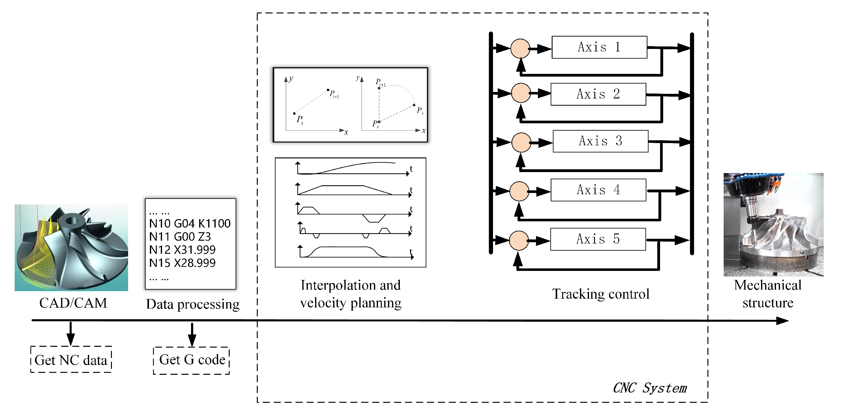
The overall architecture of CNC system processing is shown in Figure 1. Firstly, the processed NC data are generated from the CAD/CAM software model, generating G codes that the CNC system can read. NC data only contain planned position information of each axis without speed information. The CNC system performs speed planning according to the position input, sends it to each single-axis servo system, and controls the movement by servo controller so that the machine tool can run the planned path smoothly.
In order to improve machining accuracy, many studies have proposed solutions to reduce machine tools’ geometric, installation, thermal, and tool wear errors [1,2,3]. In addition, some scholars indirectly reduce the contour error by controlling the tracking error [4,5]. Different from these indirect control methods, direct contour error control is proved to be an effective method to improve the machining accuracy. In order to reduce the contour error, it is necessary to establish an accurate error estimation method. When only contour error of the translation axis is considered, Koren proposed a contour error estimation method for linear and circular trajectories [6]. Wang et al. proposed a spatial contour error estimation method based on the double Taylor expansion, and the contour error is represented by the third-order Taylor equation [7]. Wang et al. approximated the contour error based on the close circle [8]. Considering the influence of the rotation axis, Uchiyama et al. defined the five-axis contour error as tool tip position contour error and tool orientation contour error [9]. The tool tip position contour error is defined as the minimum distance between the actual trajectory and the planning trajectory, and the tool orientation contour error depends on the tool orientation deviation at the minimum tool tip position distance. On this basis, Yang et al. used a generalized Jacobian function and interpolated position commands to estimate the contour error [10]. Yang et al. proposed a on-line estimation algorithm based on three-point arc approximation and proved the method has higher estimation accuracy than linear segment approximation (LSA) algorithm [11]. Li et al. based on the synchronization of planned trajectory and actual trajectory, proposed a curve approximation method with an adaptive moving window to achieve accurate tool position and orientation contour error estimation [12]. In terms of contour error control, Wang et al. proposed a method combining iterative learning and control, using variable-gain sliding mode control to adaptively compensate for the unknown dynamics of matching in the time domain and applying an iterative learning law to suppress the influence of uncertainties [13]. Li et al. proposed a spatial iterative learning algorithm for the application scenario of large-scale repeated processing [12]. Yang et al. proposed a series of contour error compensation algorithms for cross-coupled iterative learning [14]. Altintas et al. predicted the tracking error on each feed drive as a linear function of the tangential feed, estimating and constraining the corresponding tool tip position and tool orientation errors by scaling the feed along the tool path [15]. Hu et al. used the GRU neural network as a feedforward controller to compensate for the reference contour to improve the final contour performance [16].
The methods above reduced the contour error to a certain extent; however, there are still some problems with the above methods. First, whether it is based on tracking error projection approximation or small line segment or curve equation fitting approximation, all the methods need to know the planning trajectory since it is synchronized with the actual trajectory. Only under this condition can the area for contour error estimation be determined. Second, all the methods only consider the shortest distance and ignore the influence of shape, and that will lead to estimation deviation at the large curvature trajectory. More details are described in Section 3 below. Moreover, the above methods often need to obtain the underlying controller information of the CNC machine and modify the speed planning module and closed-loop control algorithm inside the CNC system to achieve high-precision compensation. However, it is usually unrealistic for ordinary commercial CNC systems to obtain the underlying controller information and modify the controller parameters. The methods involving the underlying control are often difficult to implement due to the packaging characteristics of the CNC system.
In order to make the compensation algorithm have better versatility and operability, this paper proposes a contour error control method based on iterative learning control (ILC) by optimizing the machining NC data. Instead of using the planning trajectory, this paper proposes a contour error estimation algorithm using the planning path parsed by NC code. According to the actual single-axis motion collected by the external sensor, it is reversely mapped to the planning path. In the mapping process, the influence of trajectory shape is considered. In the process of contour error estimation, the influence weight of tool position and direction on contour error estimation is comprehensively considered in combination with the changing trend of tool position and direction, which improves the problem of ignoring the influence of tool direction in previous algorithms. The contour error is compensated offline through proportional ILC to obtain a new machining path. The contour accuracy is improved through multiple iterations only by modifying the processing commands instead of changing the underlying controller parameters, which is easier to implement in industrial applications.

2. Kinematics Model of Five-Axis CNC Machine Tool

The contour error is defined in the workpiece coordinate system, that is, the Cartesian coordinate system, but the NC data are usually a set of displacement coordinates of the servo axis in the axis coordinate system. For a two-axis or three-axis system, the conversion relationship between the axis space motion and the workpiece space motion is usually linear, and the conversion is simple. However, since the five-axis CNC system has two rotation axes, the transformation between axis space and workpiece space coordinates are usually non-linear. They have different mapping relationships depending on the structure of the machine tool.
In order to obtain the planned path in the workpiece coordinate system through NC data, it is necessary to establish the kinematics model of the CNC system to obtain the conversion relationship between the axis coordinate system and the workpiece coordinate system. Take the BC-type machine tool shown in Figure 2 below as an example. There are two rotation axes, two translation axes on the worktable, and one translation axes on the tool side. The kinematics of the CNC machine tool with this structure can be obtained using the D-H parameter method.
The positive kinematics solution of a five-axis CNC machine tool is to deduce the position and direction of the tool in the workpiece coordinate under the condition of knowing the feeds of each axis and the structural parameters of the machine tool. For example, in the machine tool with the structure shown in Figure 2, under the condition of knowing h, H and the position coordinates M = x , y , z , θ b , θ c T of the five axes, the D-H model is used to calculate the tool tip position P = [ P x , P y , P z ] T and the direction of the tool orientation in the workpiece coordinate system O = [ O i , O j , O k ] T .
The kinematics positive solution model can be obtained by the D-H parameter method, as shown in (1) and (2).
P x P y P z 1 = x cos θ b cos θ c y sin θ c + ( z + H ) sin θ b cos θ c x cos θ b cos θ c y cos θ c + ( z + H ) sin θ b sin θ c x sin θ b + ( z + H ) cos θ b h 1
O i O j O k 0 = sin θ b cos θ c sin θ b sin θ c cos θ b 0
In addition to the kinematics positive solution, after the compensation is completed, the modified trajectory in the workpiece coordinate system also needs to be converted into the NC code of the single-axis position. Therefore, it is necessary to derive the position in the axis coordinate system when the position and orientation in the workpiece coordinate system are known. The inverse kinematics solution can be obtained as (3).
θ b = arccos ( O k ) θ c = arctan 2 ( O j , O i ) x = P x cos θ b cos θ c + P y cos θ b sin θ c P z sin θ b h sin θ b y = P x sin θ c + P y cos θ c z = P x cos θ b + P y sin θ b sin θ c + P z cos θ b + h cos θ b H
Thus, according to the machine’s forward and inverse kinematics solution model, the transformation problem between the NC data in the axis coordinate system and the trajectory data in the workpiece coordinate system is solved.

3. Contour Error Estimation

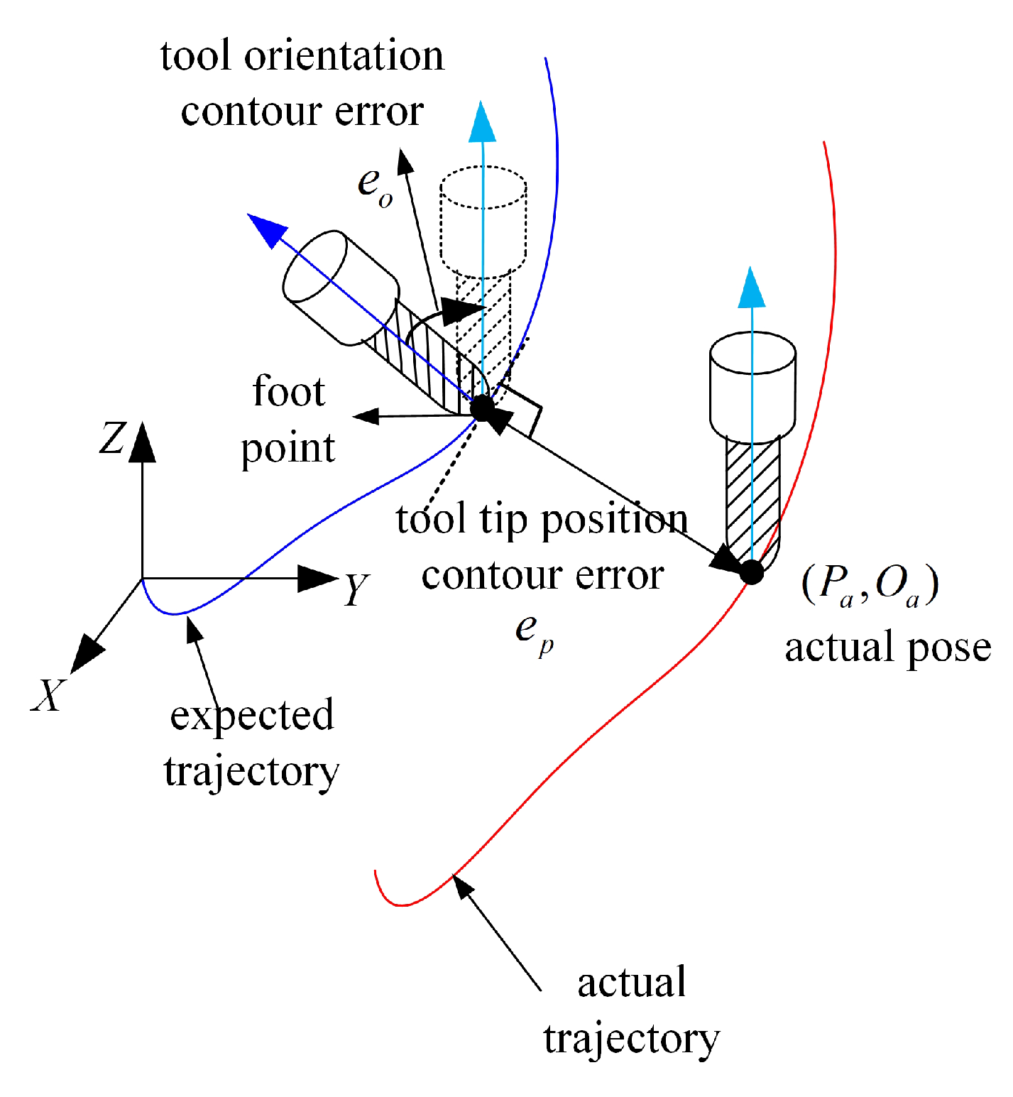
The current definition for the contour error of five-axis machine tools was proposed by Uchiyama et al. [9]. As shown in Figure 3, the tool tip position contour error is defined as the shortest distance from the actual tool tip position to the expected path. The point on the expected path closest to the actual point is called the foot point. The tool orientation contour error is defined as the angular deviation between the actual tool orientation and the tool orientation at the foot point.
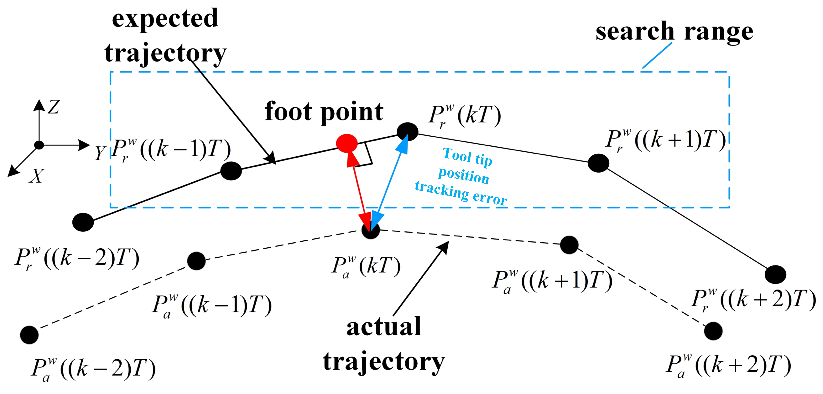
However, the five-axis contour error estimation method based on NC data cannot use the definition above directly because of the following problems. First, when knowing the expected trajectory, it can be easy to roughly determine the expected trajectory range used to find the foot point, as is shown in Figure 4. However, there is no obvious mapping relationship between points on the expected path (obtained from NC data) and points on the actual trajectory (collected by sensors), so finding the foot point can be difficult.
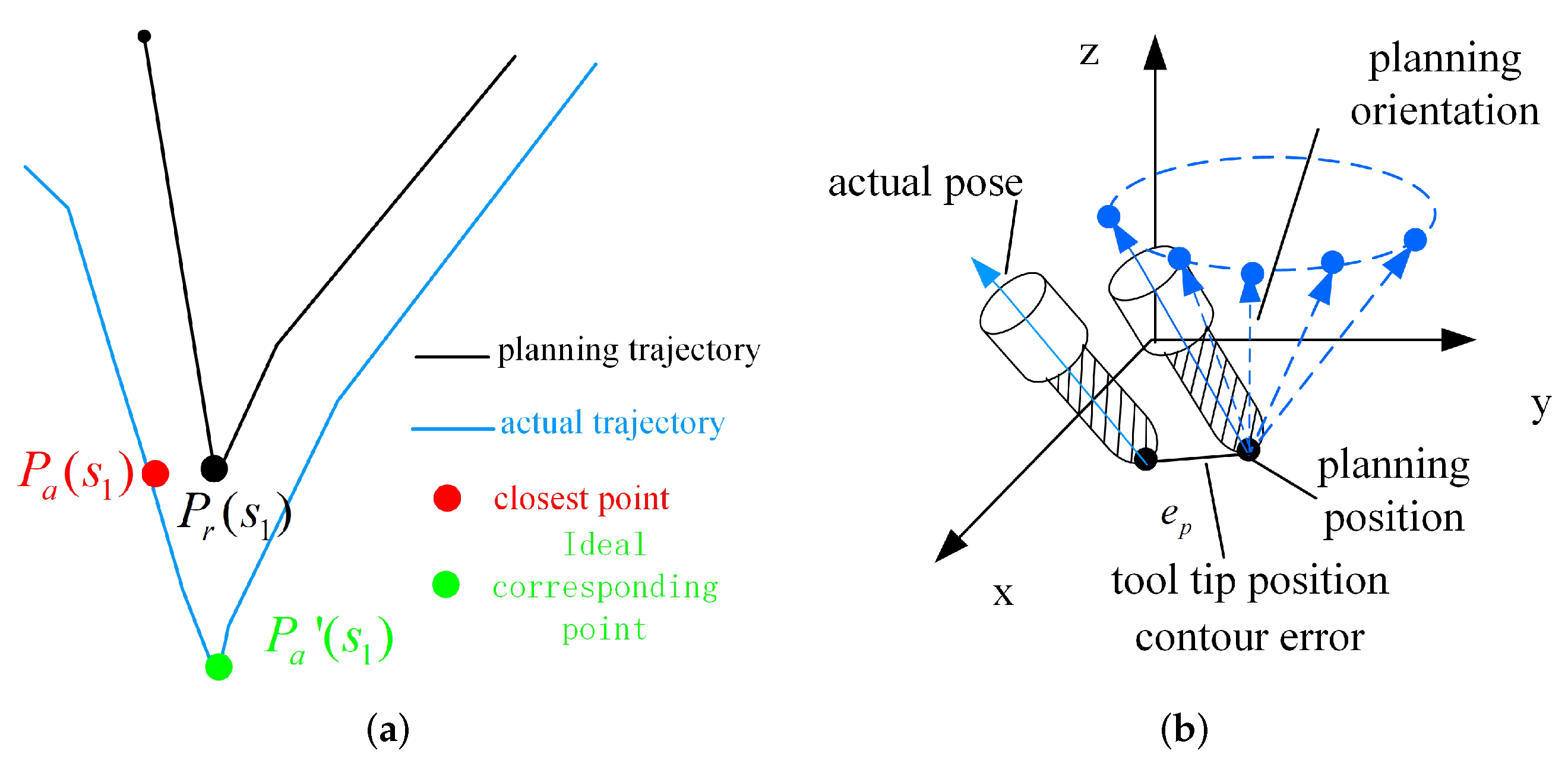
Second, the current definition only takes the tool tip position distance as the evaluation index and ignores the geometric features. For example, as shown in Figure 5a, P a ( s 1 ) is the closest actual point to P r ( s 1 ) , but considering the shape of trajectory, P a ( s 1 ) is more appropriate.
Third, for a trajectory where the tool tip position changes slightly but the tool orientation changes sharply, the current estimation method will become inaccurate. As shown in Figure 5b, the foot point is not unique, so it is unable to calculate the tool orientation contour error.
Therefore, this paper improves the current estimation method into a hybrid form to solve the problems above.

3.1. Establishment of Spatial Mapping Relationship Based on Hidden Markov Model

Before calculating the contour error, we need to establish a mapping relationship between actual trajectory and expected path so that we can determine the range of finding foot points. In this paper, we uses the hidden Markov model to map the actual trajectory points to the expected path segment.
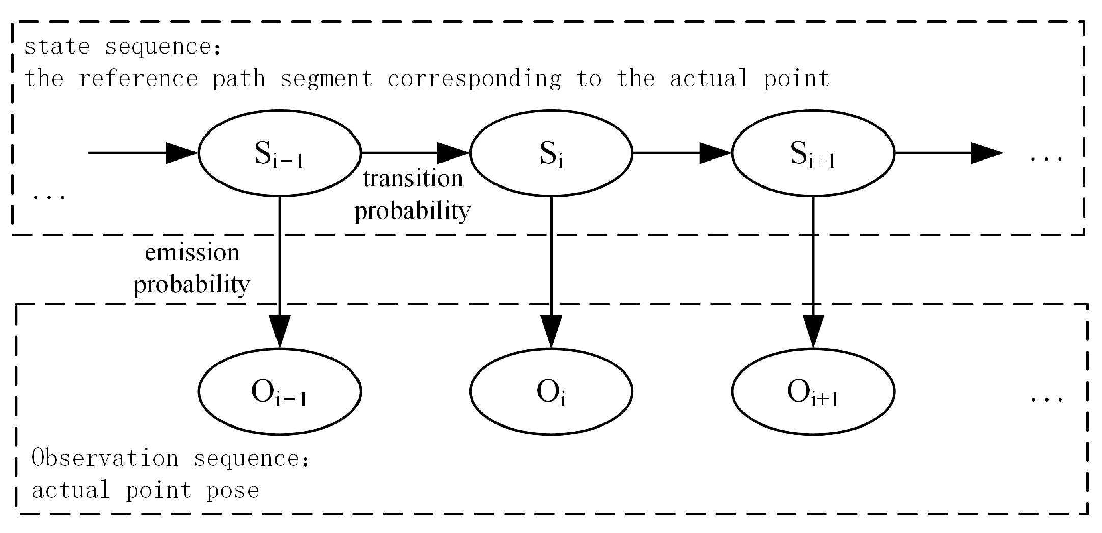
In this application, the discrete points of the actual trajectory are regarded as the observation sequence { O 1 , . . . , O n } , the expected path segment is regarded as the state sequence { S 1 , . . . , S n } . One of the fundamental problems that the hidden Markov model can solve is estimating the state sequence with the highest probability under the premise of knowing the observation sequence, emission probability, and transition probability, so it can obtain the most possible sequence of the expected path segment corresponding to the actual points. The model structure is shown in Figure 6.
In this model, the transition probability refers to the probability of transferring from one state to another state, and the emission probability refers to the probability that the state corresponds to the observation. Based on empirical considerations, the closer the actual point is to the expected path segment, the more possible it is that it corresponds to the segment. So, the emission probability is mainly based on the distance between the actual point and the expected path. Considering the geometric characteristics of the path, the probability of transferring from one segment to the next segment depends on the derection of the path and point’s movement. The transition probability depends on the sum of the deviations between the motion direction of actual points and the possible corresponding path. The specific calculation method is as follows.
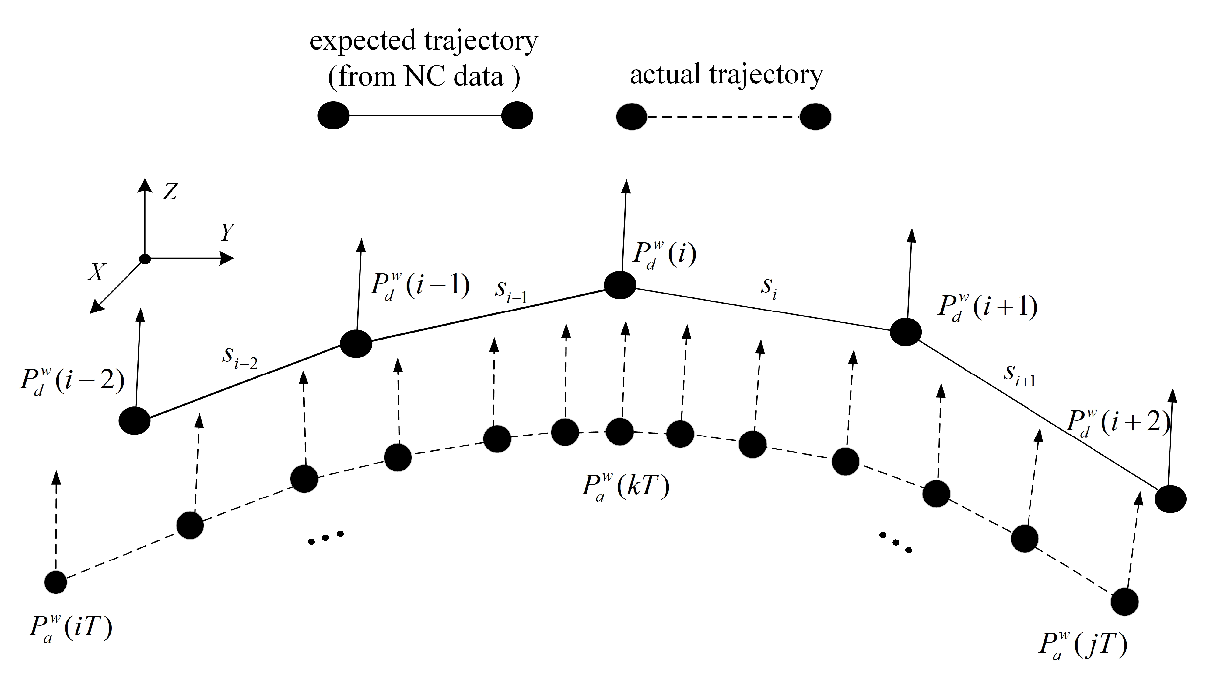
As shown in Figure 7, assume that the sensor takes T as the sampling period. The actual points are { P a w ( 0 ) , P a w ( T ) , . . . P a w ( n T ) } . The discrete points { P d w ( 1 ) , P d w ( 2 ) , . . . P d w ( m ) } on the expected path have only order but no time stamp. Here, we represent segment P d w ( i ) P d w ( i + 1 ) with s i and represent the segment corresponding to P a w ( k T ) with s ( k ) . According to the hidden Markov model, (4) expresses the probability that all actual points correspond to the possible expected path. The expected path sequence with the maximal probability calculated by (4) is the sequence that the actual points sequence corresponds to.
Π i = 1 n Pr ( P a w ( k T ) | s ( k ) ) · Π i = 1 n Pr ( s ( k ) | s ( k 1 ) )
In (4), the first part Pr ( P a w ( k T ) | s ( k ) ) represents the probability that the actual point P a w ( k T ) corresponds to s ( k ) . The second part Pr ( s ( k ) | s ( k 1 ) ) is the transition probability. Among them, s ( k ) and s ( k 1 ) may be the same segment or two adjacent segments. k only means that is corresponding to the actual point at the moment k T .
Since the probability range is [ 0 , 1 ] , multiplying multiple probabilities may result in overflow or inaccurate results. Therefore, this paper uses cost instead of probability such that the problem of finding the expected path sequence with the maximal probability is transformed into the problem of finding the expected path sequence with the minimum cost.
The emission cost is defined as the distance from the actual point to the expected path. C v ( k , i ) indicates that the cost of s ( k ) corresponding to the actual point P a w ( k T ) is the expected path s i . v represents that it is the emission cost. Its formula is shown in (5):
C v ( k , i ) = C ( P a w ( k T ) | s i ) = d i s ( P a w ( k T ) , s i ) .
The transition cost is denoted by C t ( i , j ) , where i , j indicates that the expected path segment corresponding to P a w ( k T ) is s i , and the expected path segment corresponding to P a w ( ( k 1 ) T ) is s j . Its formula is shown in (6):
C t ( i , j ) = C ( s ( k ) | s ( k 1 ) ) = C ( s i | s j ) = θ k 1 , j + θ k , i .
Among them, θ k , i is the angle difference between the motion direction of the actual point P a w ( k T ) and its corresponding path s ( k ) . In the example in Figure 8, corresponding path s ( k ) is s i .
It is assumed that the first actual point P a w ( 0 ) corresponds to the first segment s 0 , so s ( 0 ) = s 0 . Then the second actual point P a w ( T ) has two possible situation. One is that P a w ( T ) corresponds to the same segment as P a w ( 0 ) , i.e., both of them correspond to s 0 . In this case, s ( 1 ) = s 0 . The other is that P a w ( T ) corresponds to the next segment of s 0 , i.e., P a w ( T ) corresponds to s 1 . In this case, s ( 1 ) = s 1 . The costs of the two corresponding sequences can be calculated separately.
In the first case: both P a w ( 0 ) and P a w ( T ) correspond to s 0 , and the cost is shown in (7), where C ( P a w ( T ) | s 0 ) is the distance from point P a w ( T ) to segment s 0 , C ( s 0 | s 0 ) is the sum of the two angles, i.e., θ 0 , 0 and θ 1 , 0 , θ 0 , 0 is the angle difference between the motion direction of P a w ( 0 ) and the direction of s 0 , and θ 1 , 0 is the angle difference between the motion direction of P a w ( T ) and the direction of s 0 .
C v ( 1 , 0 ) · C t ( 0 , 0 ) = C ( P a w ( T ) | s 0 ) C ( s 0 | s 0 )
Second possible case: P a w ( 0 ) corresponds to s 0 , and P a w ( T ) corresponds to s 1 . The cost, in this case, is shown in (8). Where C ( P a w ( T ) | s 1 ) is the distance from point P a w ( T ) to line segment s 1 ; C ( s 1 | s 0 ) is the sum of two angles, i.e., θ 0 , 0 and θ 1 , 1 , θ 0 , 0 is the angle difference between the motion direction of point P a w ( 0 ) and the direction of line segment s 0 , and θ 1 , 1 is the angle difference between the motion direction of point P a w ( T ) and the direction of line segment s 1 .
C v ( 1 , 1 ) · C t ( 1 , 0 ) = C ( P a w ( T ) | s 1 ) C ( s 1 | s 0 )
Next, continue to calculate the segment that P a w ( 2 T ) may correspond to. In the first case above, there are two corresponding situations: P a w ( 2 T ) and P a w ( T ) correspond to the same segment s 0 or P a w ( 2 T ) corresponds to the next segment of P a w ( T ) , s 1 . In the second case above, there are also two situations: P a w ( 2 T ) and P a w ( T ) correspond to the same segment s 1 or P a w ( 2 T ) corresponds the next segment of P a w ( T ) , s 2 . From this, calculate all possible planned path segment costs when reaching P a w ( 2 T ) .
When P a w ( 0 ) , P a w ( T ) , P a w ( 2 T ) correspond to the expected path sequence s 0 , s 0 , s 0 , this sequence is under the condition of the first corresponding case of P a w ( T ) above, and its cost is shown in (9), where C v ( 1 , 0 ) · C t ( 0 , 0 ) can be obtained from (7).
C v ( 1 , 0 ) · C t ( 0 , 0 ) · C v ( 2 , 0 ) · C t ( 0 , 0 ) = C v ( 1 , 0 ) · C t ( 0 , 0 ) · C ( P a w ( 2 T ) | s 0 ) · C ( s 0 | s 0 )
When P a w ( 0 ) , P a w ( T ) , P a w ( 2 T ) correspond to the expected path sequence s 0 , s 0 , s 1 , this sequence is also under the condition of the first corresponding case of P a w ( T ) above, and its cost is shown in (10).
C v ( 1 , 0 ) · C t ( 0 , 0 ) · C v ( 2 , 1 ) · C t ( 1 , 0 ) = C v ( 1 , 0 ) · C t ( 0 , 0 ) · C ( P a w ( 2 T ) | s 1 ) · C ( s 1 | s 0 )
When P a w ( 0 ) , P a w ( T ) , P a w ( 2 T ) correspond to the expected path sequence s 0 , s 1 , s 1 , this sequence is under the condition of the second corresponding case of P a w ( T ) above, and its cost is shown in (11).
C v ( 1 , 1 ) · C t ( 1 , 0 ) · C v ( 2 , 1 ) · C t ( 1 , 1 ) = C v ( 1 , 1 ) · C t ( 1 , 0 ) · C ( P a w ( T ) | s 1 ) · C ( s 1 | s 1 )
When P a w ( 0 ) , P a w ( T ) , P a w ( 2 T ) correspond to the expected path sequence s 0 , s 1 , s 2 , this sequence is also under the condition of the second corresponding case of P a w ( T ) above, and its cost is shown in (12).
C v ( 1 , 1 ) · C t ( 1 , 0 ) · C v ( 2 , 2 ) · C t ( 2 , 1 ) = C v ( 1 , 1 ) · C t ( 1 , 0 ) · C ( P a w ( 2 T ) | s 2 ) · C ( s 2 | s 1 )
For a five-axis CNC system, another point is selected to consider the influence of the tool orientation. For example, for point Q a w ( k T ) shown in Figure 9, calculate the distance and direction deviation between it and point Q d w ( i ) on the expected tool orientation to form a line segment. When calculating the emission cost and transition cost, (13) and (14) are used for calculation.
C v ( k , i ) = d i s ( P a w ( k T ) , s i ) + d i s ( Q a w ( k T ) , q i )
C t ( i , j ) = ( θ k 1 , j + θ k , i ) + ( β k 1 , j + β k , i )
Finally, the Vertibe algorithm can calculate the sequence with the maximal probability. In this case, a certain mapping relationship can be established between the actual point and the expected path. Then the contour error can be calculated based on the contents of this section.

3.2. Tool Tip Position and Tool Orientation Contour Error Estimation

To address the problem that the current contour error estimation algorithm uses the closest tool tip position as the basis to calculate the overall contour error, this paper proposes an evaluation function that comprehensively considers the influence of tool tip position and orientation. The evaluation function is shown in (15). When calculating the contour error at a reference point, the actual point for calculating the contour error is no longer determined by the minimum tool tip position distance, but by the minimum evaluation function.
F = K p | e p | + K o e o · R
In (15), e p and e o are the tool tip position and tool orientation deviation from a reference point to a actual point and | e p | is the modulus of e p . K p and K o are two coefficients change with the changing trend of the tool tip position and tool orientation. If the position of the tool tip changes sharply, K p will be larger, and e p plays a major role in (15). Otherwise, K o will be larger, and F is mainly affected by e o . Since the dimensions and magnitudes of the two deviations of e p and e o are not uniform, the coefficient R is used for adjustment. The calculation method of the above coefficients is described below.
As shown in Figure 10, the tool tip position changing speed at the reference point P a w ( k T ) can be estimated as (16). Tool orientation changing speed can be calculated by (17).
v d w ( i ) = P a w ( k T ) P a w ( ( k 1 ) T ) + P a w ( k T ) P a w ( ( k + 1 ) T ) 2 T
θ ˙ d ( i ) = Δ θ a ( k T ) + Δ θ a ( ( k + 1 ) T ) 2 T
In the workpiece coordinate, the tool tip position coordinates of point P a w ( k T ) can be expressed as P a w ( k T ) = [ P a x ( k T ) , P a y ( k T ) , P a z ( k T ) ] , and the tool orientation vector is expressed as O a w ( k T ) = [ O a i ( k T ) , O a j ( k T ) , O a k ( k T ) ] , P a w ( k T ) P a w ( ( k 1 ) T ) in (16) can be calculated by (18) and Δ θ a ( k T ) can be calculated by (19).
P a w ( k T ) P a w ( ( k 1 ) T ) = | P a w ( k T ) P a w ( ( k 1 ) T ) |
Δ θ a ( k T ) = arccos ( O a ( ( k 1 ) T ) · O a ( k T ) )
Finally, the coefficients are normalized, and the parameters K p and K o are calculated using (20) and (21), respectively. Finally, the coefficient R is determined according to the tool position and orientation changes of the machining reference path. So far, all the parameters in (15) except the angle deviation e o and distance deviation e p have been obtained.
K o = θ ˙ d ( i ) · R θ ˙ d ( i ) · R + v d w ( i )
K p = v d w ( i ) θ ˙ d ( i ) · R + v d w ( i )
In Section 3.1, each actual point corresponds to the expected path segment. As shown in Figure 10, assume that all points between point P a w ( ( k m ) T ) and P a w ( k T ) correspond to the reference path segment P d w ( i 1 ) P d w ( i ) , and points P a w ( ( k + 1 ) T ) to P a w ( ( k + n ) T ) correspond to the reference path segment P d w ( i ) P d w ( i + 1 ) . Then, when calculating the contour error of P d w ( i ) , the estimation range is narrowed down to the actual points corresponding to the adjacent segments of P d w ( i ) . For example, for P d w ( i ) , actual points P a w ( ( k 1 ) T ) , P a w ( k T ) , and P a w ( ( k + 1 ) T ) respectively correspond to segments P d w ( i 1 ) P d w ( i ) and P d w ( i ) P d w ( i + 1 ) . We select P a w ( ( k 1 ) T ) , P a w ( k T ) , and P a w ( ( k + 1 ) T ) to fit the actual trajectory with a quadratic polynomial. Taking the x-axis as an example, when the x-axis displacements corresponding to P a w ( ( k 1 ) T ) , P a w ( k T ) , and P a w ( ( k + 1 ) T ) are x a ( k 1 ) , x a k , and x a ( k + 1 ) , respectively, the fitting is performed with a quadratic polynomial:
x a ( t ) = a x 1 t 2 + a x 2 t + a x 3 .
Substitute t = k , k 1 , k + 1 into (23) to obtain (23).
( k 1 ) 2 k 1 1 k 2 k 1 ( k + 1 ) 2 k + 1 1 a x 1 a x 2 a x 3 = x a ( k 1 ) x a k x a ( k + 1 )
Substitute the coordinates of each point and (23) can be solved:
a x 1 = x a ( k 1 ) 1 × ( 2 ) + x a k 1 × ( 1 ) + x a ( k + 1 ) 2 × 1 a x 2 = ( k + k + 1 ) x a ( k 1 ) 1 × 1 + ( k + 1 + k 1 ) x a k 1 × ( 1 ) + ( k 1 + k ) x a ( k + 1 ) 1 × 1 a x 3 = k ( k + 1 ) x a ( k 1 ) 1 × 1 + ( k + 1 ) ( k 1 ) x a k 1 × ( 1 ) + ( k 1 ) k x a ( k + 1 ) 1 × 1
Therefore, the actual trajectory from P a w ( ( k 1 ) T ) to P a w ( ( k + 1 ) T ) is decomposed to the x-axis and can be fitted by (21), and the fitting parameters can be obtained. Similarly, the above methods can solve the fitting equations of the actual points P a w ( ( k 1 ) T ) to P a w ( ( k + 1 ) T ) in the sliding window interval corresponding to the reference point P d w ( i ) for other axes.
x a ( t ) = a x 1 t 2 + a x 2 t + a x 3 y a ( t ) = a y 1 t 2 + a y 2 t + a y 3 z a ( t ) = a z 1 t 2 + a z 2 t + a z 3 b a ( t ) = a b 1 t 2 + a b 2 t + a b 3 c a ( t ) = a c 1 t 2 + a c 2 t + a c 3
After substituting (25) into the kinematics forward solution conversion formula obtained from the machine tool structure, the tool tip position and tool orientation of the actual trajectory used to calculate contour error can be converted into a function of t. The tool tip position coordinates and tool orientation vectors of the trajectory between the actual point P a w ( ( k 1 ) T ) and P a w ( ( k + 1 ) T ) in the workpiece coordinate can be expressed as: [ P a x ( t ) , P a y ( t ) , P a z ( t ) , O a i ( t ) , O a j ( t ) , O a k ( t ) ] , i.e., a function with t as a variable.
For each reference point P d w ( i ) , the actual trajectory for calculating the contour error can be expressed. Then, the position distance from the current reference point to the trajectory can be calculated by (27), (26) can represent the tool orientation deviation from the current reference point to the actual trajectory.
e o ( t ) = arccos ( O d i , i · O a , i ( t ) + O d i , j · O a , j ( t ) + O d i , k · O a , k ( t ) )
e p ( t ) = [ P d x ( i ) , P d y ( i ) , P d z ( i ) ] [ P a x ( t ) , P a y ( t ) , P a z ( t ) ]
After substituting (26) and (27) into (15), the current evaluation function can be expressed as an expression with t as the variable shown in (28).
F ( t ) = K o e o ( t ) · R + K p e p ( t )
Calculate the value of t to the minimum evaluation function and get t m i n . Take t m i n into (24) and (23). The obtained e o ( t m i n ) and e p ( t m i n ) are the tool orientation and tool tip position contour errors at the reference point. If the reference point is P d w ( i ) ) , the tool orientation and tool tip position contour error are denoted as e o ( i ) and e p ( i ) , respectively.

4. Contour Error Compensation Based on Iterative Learning

The contour error of the five-axis CNC system includes two parts: tool tip position contour error and tool orientation contour error. Therefore, during the compensation process, both errors need to be compensated at the same time.
The tool tip position coordinates and tool orientation vector of the initially planned path are represented by symbols P d ( i ) and O d ( i ) , respectively. The k-th reference path is P r , k w ( i ) = [ P r , k ( i ) , O r , k ( i ) ] . When k = 1 , the reference path is the expected path. In Section 3.2, the corresponding contour errors during the k-th iteration at each point are calculated, i.e., e p , k ( i ) and e o , k ( i ) .
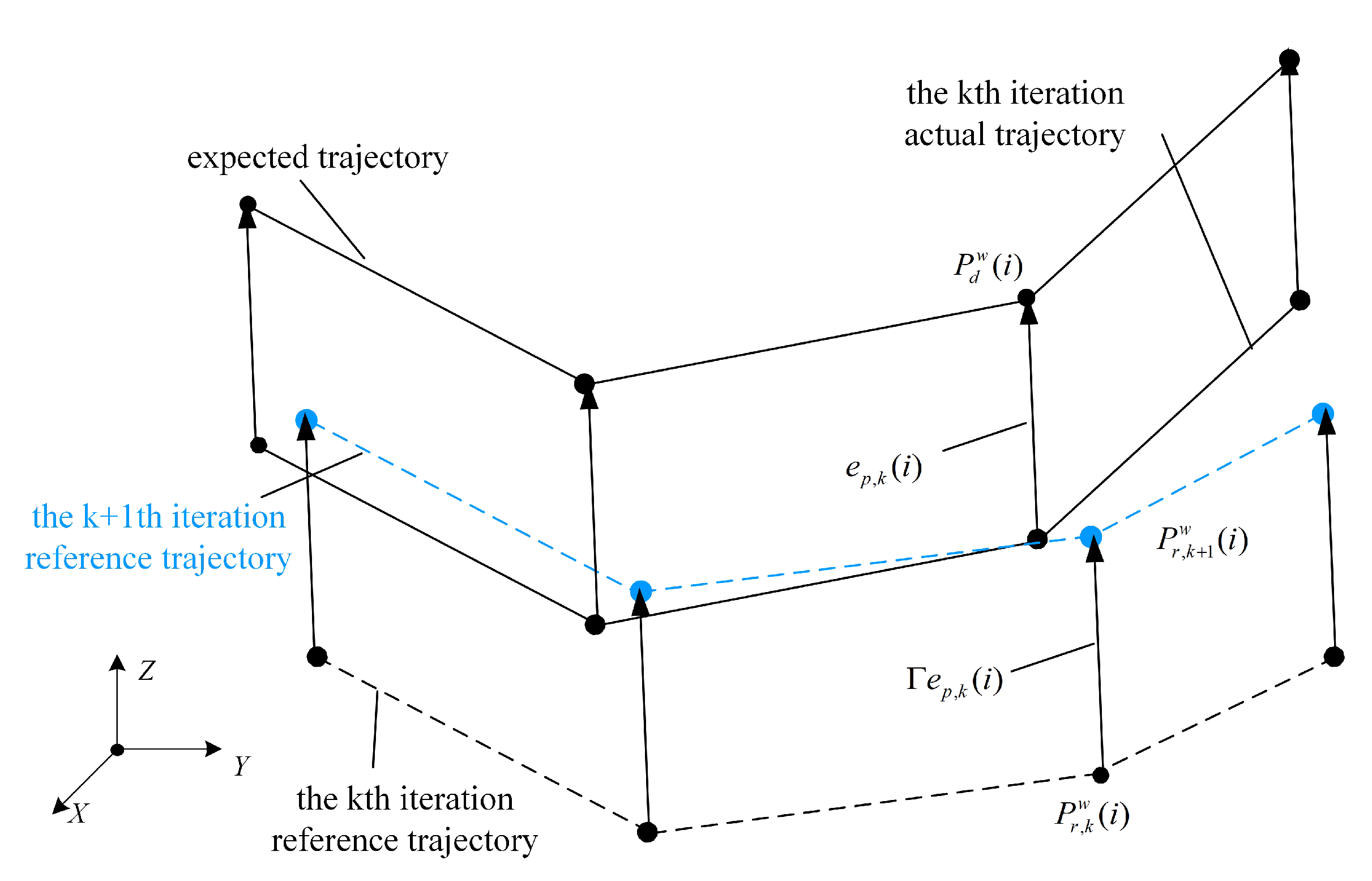
For the compensation of the tool tip position contour error, we use the method of transforming the reference path along the error direction into Cartesian space for compensation. After the first run is completed and the contour error at each reference point is calculated, the reference trajectory of the initial compensation is the expected point, i.e., P r , 1 ( i ) = P d ( i ) , and the reference trajectory of the second iteration obtained after compensation is calculated as:
P r , 2 ( i ) = P r , 1 ( i ) + Γ e p , k ( i ) .
After that, the reference path after each iteration compensation is obtained by the current reference path point along the tool tip position error transformation compensation amount, as shown in Figure 11, and the k-th iteration tool tip position contour error is shown in (27). Then the k-th tool tip position reference path is obtained by compensating Γ e p , k ( i ) into the Cartesian space for the k-th reference path, that is, P r , k + 1 w ( i ) = P r , k w ( i ) + Γ e p , k ( i ) .
The tool tip position contour error is the geometric deviation between the actual trajectory of this operation and the expected path, which is calculated by (30).
e p , k ( i ) = [ P d x ( i ) , P d y ( i ) , P d z ( i ) ] [ P a x , k ( i ) , P a y , k ( i ) , P a z , k ( i ) ]
The reference tool orientation after compensation is the last reference tool orientation rotated by Γ · e o , 1 ( i ) degrees around the cross product vector of the corresponding actual tool orientation. For the tool orientation contour error calculated for the first time, its magnitude is e o , 1 ( i ) , and the compensation direction should be rotated clockwise by the direction of the reference path along its cross-product vector with the direction at the corresponding point. As shown in Figure 12, the cross product vector B 1 ( i ) is calculated by (31).
B 1 ( i ) = [ O d i ( i ) , O d j ( i ) , O d k ( i ) ] × [ O a i , 1 ( i ) , O a j , 1 ( i ) , O a k , 1 ( i ) ]
In the first iteration, O r , 1 ( i ) = O d ( i ) , the reference tool orientation after compensation can be calculated by (32), where O d ( i ) = [ O d i ( i ) , O d j ( i ) , O d k ( i ) ] .
O r , 2 ( i ) = O r , 1 ( i ) · cos ( Γ e o , 1 ( i ) ) + ( B 1 ( i ) × O r , 1 ( i ) ) sin ( Γ e o , 1 ( i ) ) + ( B 1 ( i ) · O r , 1 ( i ) ) ( 1 cos ( Γ e o , 1 ( i ) )
The new reference tool pose is used as the input of the next iteration, and the actual operation result of the next iteration is obtained. Finally, the above process is repeated until convergence to obtain the reference input that makes the operation result closest to the expected output.
In the k-th iteration process, B k ( i ) is the cross product of the planned tool orientation O d ( i ) and the corresponding actual tool orientation O a , k ( i ) , and the basis for obtaining the k + 1 th input after compensation is the kth input:
O r , k + 1 ( i ) = O r , k ( i ) · cos ( Γ e o , k ( i ) ) + ( B k ( i ) × O r , k ( i ) ) sin ( Γ e o , k ( i ) ) + ( B k ( i ) · O r , k ( i ) ) ( 1 cos ( Γ e o , k ( i ) ) .
After the reference path of the next iteration is obtained through compensation, the compensated result needs to be transformed into each single-axis space through the kinematic inverse solution before the next iteration of operation. First, the coordinate P r , k w ( i ) of the workpiece space is converted into the coordinate P r , k d ( i ) of the servo motion axis through (34) and then further converted into the G code to obtain the next iteration’s input. The conversion relation T w d ( · ) is determined by the physical structure of the multi-axis linkage system.
P r , k d ( i ) = T w d ( P r , k w ( i ) )

5. Results and Discussion

This paper uses the B-C five-axis CNC machine tool shown in Figure 13 to verify the proposed method.
The platform is a BC-type double turntable five-axis CNC machine tool. It is equipped with a solid high CNC system, which can specify the machining contour through the host computer and output the interpolation trajectory and actual running information of the CNC system. The three linear axis drivers are Yaskawa SGDM-10ADA-V, and the two rotary axis drivers are Sanyo RS1A03AAWA. The position loop gains of the three linear axes are respectively set to K v x = 150 , K v y = 199 , K v z = 107 , and the position loop gains of the two rotary axes are respectively set to K v b = 75 , K v c = 50 . The encoder of the rotary axis is a position sensor with a resolution set to 32,768 p/r, and the motor’s pitch is 5 mm. On the controller panel, the sampling frequency is 500 Hz. In the experiment, the CNC machine tool receives the G code based on G01. The CNC system collects each axis’s planned position and actual position information.
In this section, the method proposed in this paper is compared with the algorithm proposed in article [12] to verify the progress made by the current algorithm.
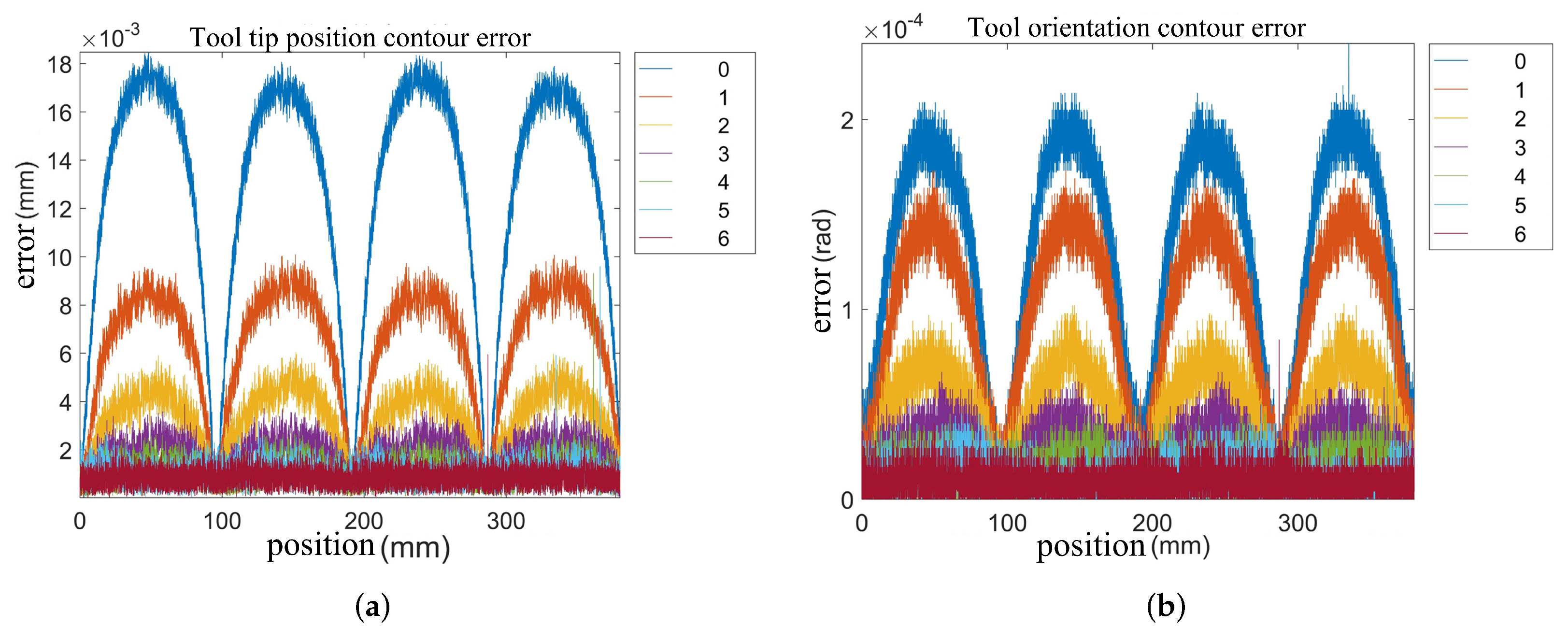
First, the contour error estimation and compensation experiment is conducted for the circular projection trajectory on the relatively smooth saddle surface, as shown in Figure 14.
The effect of iterative compensation using the error estimation method proposed in article [12], which is based on the planned trajectory and uses the nearest tool position as the profile error evaluation standard, is shown in Figure 15.
The results of contour error estimation and compensation based on NC code proposed in this paper are shown in Figure 16.
The experimental results show that for a simple trajectory, the proposed contour error estimation method using only the planning path has the same good effect on improving the contour accuracy as the method based on the planning trajectory after compensation.
Next, in order to verify the improvement of compensation effect at large curvature combined with the influence of trajectory shape, the following trajectory in Figure 17 is used for the experiment. This trajectory is the projection trajectory of flowers on the saddle surface with sharp corners of curvature. Among them, the saddle surface formula is:
z = x 2 100 y 2 100 + 200 .
The formula of the flower trajectory is:
x = Rsin ( 3 t ) + R , t [ 0 , π 2 ] Rsin ( 3 t ) R , t [ π 2 , π ] Rsin ( 3 t ) R , t [ π , 3 π 2 ] Rsin ( 3 t ) + R , t [ 3 π 2 , 2 π ] y = Rsin ( 3 t ) + R , t [ 0 , π 2 ] Rsin ( 3 t ) + R , t [ π 2 , π ] Rsin ( 3 t ) R , t [ π , 3 π 2 ] Rsin ( 3 t ) + R , t [ 3 π 2 , 2 π ] .
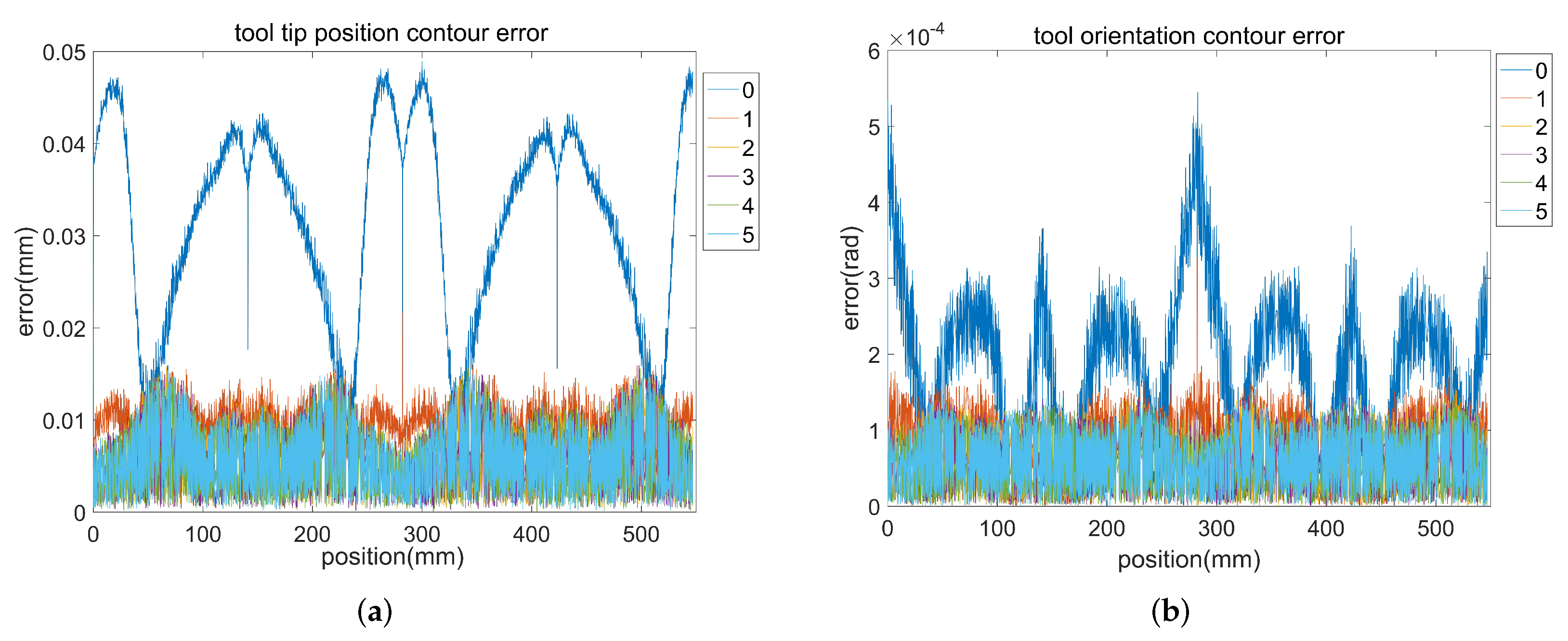
When the feed rate is 3000 mm/min, and the gain of iterative learning is 0.8 , the estimation method proposed in article [12] based on planning trajectory and take the nearest tool position distance as the evaluation index of contour error to estimate and compensate for the contour error of the flower trajectory, and the compensation results are shown in Figure 18. Among them is the change of tool tip position contour error and the tool orientation contour error with iterative compensation.
The results of iterative compensation of the contour error estimated by the algorithm based on distance are listed in Table 1. It can be seen that in the process of multiple iterations, the root mean square value of the tool tip position and tool orientation contour error is gradually decreasing, but the maximum value has increased. The experimental results show that the machining accuracy of most smooth geometric paths can be improved by using this method. However, the contour error at the sharp corners is not reduced, but divergence will appear.
Using the NC data and methods proposed in this paper, the experimental results of the contour error estimation and compensation method based on the hidden Markov model and combined the trajectory shape features and the tool position and orientation moving speed is shown in the figure are shown in Figure 19 and Table 2.
Enlargement of the sharp corner of the flower trajectory, and the results of the two methods in each iterative compensation, are shown in Figure 20.
It can be seen from the result that, after iterative compensation using the estimation method proposed in this paper, the contour error converges well on the entire trajectory, and the root-mean-square error and the maximum value both decrease steadily. The divergence phenomenon does not exist.
In CNC machining, the overall precision requirements of the processed products are very high, and the divergence of errors in a certain part of the machining will cause obvious marks on the surface of the processed parts, which will affect the performance of the parts. It can be seen that using the contour error estimation method proposed in this paper can improve the overall precision of parts processing.
To sum up, the method proposed in this paper is easier to implement on commercial CNC systems because it only needs the planning path, which can be acquired by NC code instead of the planning trajectory. For simple trajectory, the algorithm proposed in this paper has the same good control effect as the traditional algorithm. At the same time, because the influence of trajectory motion shape is considered in the establishment of hidden Markov model mapping relationship, and the influence of tool position and direction is comprehensively considered in the process of contour error estimation, the estimation algorithm proposed in this paper is more difficult to produce divergence after compensation at the large curvature trajectory.

6. Conclusions

This paper proposes a contour error estimation method based on NC codes combined with trajectory geometry features. This method avoids the need for planning trajectory in traditional contour error estimation algorithm, and has better industrial feasibility. Using the Hidden Markov Model, the spatial mapping relationship between the actual trajectory and the planning path is established, and a new method for contour error estimation is proposed. Compared with the existing methods, this method has higher estimation accuracy at some sharp corner trajectories. The results show that the method proposed in this paper has wider applicability and practical significance for improving the precision of NC machining.

Author Contributions

Conceptualization, J.L.; methodology, J.L. and R.Y.; software, R.Y.; validation, J.L., R.Y. and Y.F.; formal analysis, R.Y.; investigation, R.Y.; resources, J.L., R.Y. and Y.F.; data curation, R.Y.; writing—original draft preparation, R.Y.; writing—review and editing, J.L. and Y.F.; visualization, R.Y. and Y.F.; supervision, J.L.; project administration, J.L.; funding acquisition, J.L. All authors have read and agreed to the published version of the manuscript.

Funding

This research was funded by Shenzhen Science and Technology Program grant number GXWD20201230155427003-20200821171505003 and in part by the National Natural Science Foundation of China grant number 52275481.

Data Availability Statement

Data will be made available from the corresponding author on reasonable request.

Conflicts of Interest

The authors declare no conflict of interest. The funders had no role in the design of the study; in the collection, analyses, or interpretation of data; in the writing of the manuscript; or in the decision to publish the results.

References

  1. Cheng, Y.; Zhang, X.; Zhang, G.; Jiang, W.; Li, B. Thermal deformation analysis and compensation of the direct-drive five-axis CNC milling head. J. Mech. Sci. Technol. 2022, 36, 4681–4694. [Google Scholar] [CrossRef]
  2. Liu, J.; Ma, C.; Gui, H.; Wang, S. Thermally-induced error compensation of spindle system based on long short term memory neural networks. Appl. Soft Comput. 2021, 102, 107094. [Google Scholar] [CrossRef]
  3. Niu, P.; Cheng, Q.; Liu, Z.; Chu, H. A machining accuracy improvement approach for a horizontal machining center based on analysis of geometric error characteristics. Int. J. Adv. Manuf. Technol. 2021, 112, 2873–2887. [Google Scholar] [CrossRef]
  4. Altintas, Y.; Erkorkmaz, K.; Zhu, W.H. Sliding mode controller design for high speed feed drives. CIRP Ann. 2000, 49, 265–270. [Google Scholar] [CrossRef]
  5. Xie, Z.; Xie, F.; Liu, X.J.; Wang, J.; Mei, B. Tracking error prediction informed motion control of a parallel machine tool for high-performance machining. Int. J. Mach. Tools Manuf. 2021, 164, 103714. [Google Scholar] [CrossRef]
  6. Koren, Y. Cross-coupled biaxial computer control for manufacturing systems. J. Dyn. Syst. Meas. Control. 1980, 102, 265–272. [Google Scholar] [CrossRef]
  7. Wang, Z.; Hu, C.; Zhu, Y. Double taylor expansion-based real-time contouring error estimation for multiaxis motion systems. IEEE Trans. Ind. Electron. 2019, 66, 9490–9499. [Google Scholar] [CrossRef]
  8. Wang, J.; Sui, Z.; Tian, Y.T.; Wang, X.; Fang, L. A speed optimization algorithm based on the contour error model of lag synchronization for CNC cam grinding. Int. J. Adv. Manuf. Technol. 2015, 80, 1421–1432. [Google Scholar] [CrossRef]
  9. Uchiyama, N.; Ahmad-Mohammad, A.-E.-K.M. Estimation of tool orientation contour errors for five-axismachining. Robot.-Comput.-Integr. Manuf. 2013, 29, 271–277. [Google Scholar]
  10. Yang, J.; Altintas, Y. A generalized on-line estimation and control of five-axis contouring errors of CNC machine tools. Int. J. Mach. Tools Manuf. 2015, 88, 9–23. [Google Scholar] [CrossRef]
  11. Yang, M.; Yang, J.; Ding, H. A high accuracy on-line estimation algorithm of five-axis contouring errors based on three-point arc approximation. Int. J. Mach. Tools Manuf. 2018, 130, 73–84. [Google Scholar] [CrossRef]
  12. Li, J.; You, Z.; Li, Y.; Miao, E.; Yue, R. Five-Axis Contour Error Control Based on Spatial Iterative Learning. IEEE Trans. Autom. Sci. Eng. 2023, 20, 112–123. [Google Scholar] [CrossRef]
  13. Wang, W.; Ma, J.; Cheng, Z.; Li, X.; de Silva, C.W.; Lee, T.H. Global iterative sliding mode control of an industrial biaxial gantry system for contouring motion tasks. IEEE/ASME Trans. Mechatron. 2021, 27, 1617–1628. [Google Scholar] [CrossRef]
  14. Yang, J.; Li, J.; Liu, Z.; Zhang, T. Cross-coupled iterative learning contour compensation for high speed motion based on modified reference input. In Proceedings of the IEEE 2018 Chinese Automation Congress (CAC), Xi’an, China, 30 November–2 December 2018; pp. 1778–1783. [Google Scholar]
  15. Altintas, Y.; Yang, J.; Kilic, Z.M. Virtual prediction and constraint of contour errors induced by cutting force disturbances on multi-axis CNC machine tools. CIRP Ann. 2019, 68, 377–380. [Google Scholar] [CrossRef]
  16. Hu, C.; Ou, T.; Chang, H.; Zhu, Y.; Zhu, L. Deep GRU neural network prediction and feedforward compensation for precision multiaxis motion control systems. IEEE/ASME Trans. Mechatron. 2020, 25, 1377–1388. [Google Scholar]
Figure 1. CNC machining process.
Machines 11 00085 g001
Figure 2. B-C type five-axis CNC machine.
Machines 11 00085 g002
Figure 3. Traditional contour error definition.
Machines 11 00085 g003
Figure 4. Search range of foot point.
Machines 11 00085 g004
Figure 5. Existing problems of currrent estimate method. (a) Estimation error caused by current method. (b) Estimation error caused by currrent method.
Machines 11 00085 g005
Figure 6. Hidden Markov model.
Machines 11 00085 g006
Figure 7. Correspondence between actual and expected trajectories.
Machines 11 00085 g007
Figure 8. Algorithm application example.
Machines 11 00085 g008
Figure 9. Algorithm application example for 5-axis CNC.
Machines 11 00085 g009
Figure 10. Example of contour error estimation
Machines 11 00085 g010
Figure 11. Example of tool tip position contour error compensation.
Machines 11 00085 g011
Figure 12. Example of tool orientation contour error compensation.
Machines 11 00085 g012
Figure 13. NC machine tool used in the experiment.
Machines 11 00085 g013
Figure 14. Circular projection on saddle surface.
Machines 11 00085 g014
Figure 15. Contour error compensation results of circular projection on saddle surface. (a) Tool tip position contour error compensation based on the nearest distance. (b) Tool orientation contour error compensation based on the nearest distance.
Machines 11 00085 g015
Figure 16. Contour error compensation results of circular projection on saddle surface. (a) Tool tip position contour error compensation based on HMM. (b) Tool orientation contour error compensation based on HMM.
Machines 11 00085 g016
Figure 17. Flower projection on saddle surface.
Machines 11 00085 g017
Figure 18. Contour error compensation results of flower projection on saddle surface. (a) Tool tip position contour error compensation based on the nearest distance. (b) Tool orientation contour error compensation based on the nearest distance.
Machines 11 00085 g018
Figure 19. Contour error compensation results of flower projection on saddle surface. (a) Tool tip position contour error compensation based on HMM. (b) Tool orientation contour error compensation based on HMM.
Machines 11 00085 g019
Figure 20. (a) Trajectory in multiple compensation based on the nearest distance. (b) Trajectory in multiple compensation based on HMM.
Machines 11 00085 g020
Table 1. Errors in multiple compensation based on the nearest distance.
iteration e pmax ( μ m) e prms ( μ m) e omax ( 10 4 rad) e orms ( 10 4 rad)
023.7619.922.971.94
132.5917.643.681.62
239.9916.695.531.14
339.9616.315.481.06
439.8915.975.430.997
539.8515.525.310.986
623.6715.393.360.857
Table 2. Errors in multiple compensation based on HMM.
Iteration e pmax ( μ m) e prms ( μ m) e omax ( 10 4 rad) e orms ( 10 4 rad)
048.9235.465.533.94
121.3116.313.921.62
216.2415.421.511.14
316.1115.391.371.06
416.0414.981.320.961
515.9114.861.330.954
615.7914.631.310.898
Disclaimer/Publisher’s Note: The statements, opinions and data contained in all publications are solely those of the individual author(s) and contributor(s) and not of MDPI and/or the editor(s). MDPI and/or the editor(s) disclaim responsibility for any injury to people or property resulting from any ideas, methods, instructions or products referred to in the content.