Experimental Vibration Data in Fault Diagnosis: A Machine Learning Approach to Robust Classification of Rotor and Bearing Defects in Rotating Machines

Abstract

This study builds upon previous research that utilised a vibration-based machine learning (VML) approach for diagnosing rotor-related faults in rotating machinery. The original method used artificial neural networks (ANN) to classify rotor-related faults based on optimised vibration parameters from the time and frequency domains. This study expands the application of this vibration-based machine learning approach to include the anti-friction bearing faults in addition to the rotor faults. The earlier suggested vibration-based parameters, both in time and frequency domains, are further revised to accommodate bearing-related defects. The study utilises the measured vibration data from a laboratory-scale rotating test rig with different experimentally simulated faults in the rotor and bearings. The proposed VML model is developed for both rotor and bearing defects at a rotor speed that is above the first critical speed. To gauge the robustness of the proposed VML model, it is further tested at two different rotating speeds, one below the first critical speed and the other above the second critical speed. The paper presents the methodology, the rig and measured vibration data, the optimised parameters, and the findings.

1. Introduction

The operations of most industries and power plants rely significantly on rotating machinery, which makes the accurate detection of faults associated with this class of machines at early stages a vital objective. Typical rotating machines comprise several integrated components, including rotors, bearings, supporting structures, couplings, electric motors, etc. The dynamic conditions under which they operate and the manufacturing/installation imperfections make them vulnerable to various abnormalities, of which rotor and bearing-related faults are prevalent. The most common rotor faults that cause rotor vibration are rotor unbalance, rotor/coupling misalignment, and rotor-to-stator rubbing [1].

The malfunctions in rotating machinery may cause damage to the critical components of the machine, such as bearings, or even lead to machine failure, which has safety and economic implications [2]. Therefore, the early detection and reliable diagnosis of rotor and bearing faults in their preliminary stages have become essential in industries to enhance machine reliability and maintenance cost-effectiveness. Recently, manufacturing companies have made great efforts to implement effective machinery maintenance programs that can detect and diagnose rotor and bearing faults at their initial stages [3,4].

The vibration response of rotating machines is sensitive to any change in the structural parameters. Moreover, vibration behaviour due to rotor defects varies depending on the nature of the fault. Hence, analysing the vibration signals can reveal any faults in the rotating machines. Therefore, vibration-based condition monitoring (VCM) has been beneficial in detecting rotor and bearing-related faults. Generally, the VCM is done by installing several vibration sensors at individual bearing locations on the monitored machine. Over the years, VCM techniques have been successfully used to detect and diagnose rotor and bearing faults [5,6,7]. A summary of the recent research in machine diagnosis and prognosis, as well as possible future trends, has been provided by Jardine et al. [8]. Tama et al. [9] and Kumar et al. [10] have recently provided an overview of the VCM and presented a literature review on recent research in this field. Furthermore, they have built an experimental rig to simulate some rotor faults, namely rotor unbalance and shaft misalignment. A recent thorough review of vibration-based condition monitoring of rotating machinery is presented by Tiboni et al. [11]. Yunusa-Kaltungo [12] has provided a comprehensive literature review of the VCM in rotating machines.

Currently, many researchers have proposed VCM that employs artificial intelligence (AI) techniques in the rotor faults identification process, such as fuzzy logic methods and artificial neural networks (ANN) [13,14]. ANNs have shown, in many research studies in recent days, their effectiveness for accurately identifying the different rotating machine faults. Moreover, artificial intelligence methods can help accelerate decision-making with reduced human involvement.

Mubaraali et al. [15] have introduced an intelligent diagnostic system method that employs a fuzzy neural network using the special bearing diagnostic symptom parameters (SSPs) in time and frequency domains to precisely and automatically determine the fault type of low-speed bearings. Khoualdia et al. [16] have been able to diagnose faults in an induction motor under different operating conditions using a multi-layer perceptron (MLP) artificial neural network (ANN) with the Levenberg–Marquardt learning algorithm. The faults included in their study are broken rotor bars, bearing faults, and misalignment.

Sepulveda and Sinha [17] have developed a machine fault diagnosis model that can be applied blindly to similar machines with high accuracy in the predictions. They have identified the healthy and faulty conditions of an experimental rig operating at various speeds using a smart vibration-based machine learning (SVML) model. Mei et al. [18] achieved deep analysis and processing of large-scale data while selecting several feature combinations that effectively characterise state information. Their research proposes a machinery and equipment CM method combining the relative degree of contribution (RDoC)-based feature selection and deep residual network (DRN). They proposed an optimal feature combination selection strategy with high characterisation information density to meet the challenge of large numbers of sensors with mismatched sampling rates.

Espinoza-Sepulveda and Sinha [19] have presented a vibration-based ML model (VML) with a multi-layered perceptron (MLP) network, four hidden layers, and each of them with a variable quantity of non-linear neurons. Their proposed method used vibration measurements from a laboratory-scaled rig and employed an artificial intelligence (AI)-based machine learning (ML) model. The research mainly focused on optimising vibration-based parameters for identifying rotor faults without including other rotating machinery components and used the artificial neural network (ANN) model for classification. However, there is a need to investigate these parameters’ effectiveness in identifying rotor and bearing faults.

The current study is further extended from the earlier study [19]. The ANN model and the vibration parameters used in the earlier VML model [19] for rotor fault detection are used again in the current study to standardise the earlier proposed method. However, the vibration parameters [19] in both time and frequency domains are further revised by extending the frequency band so the revised parameters can cover the anti-frication bearing defects. The measured vibration data from a laboratory-scale rotating test rig with different experimentally simulated faults in the rotor and bearings are used in this study. The bearing supports for the rig are designed such that the rig can operate below and above the critical speeds. The proposed VML model is developed for both rotor and bearing defects at a rotor speed that is above the first critical speed. The proposed VML model is further tested at two different rotating speeds, one below the first critical speed and the other above the second critical speed. The dynamics of the machine are different at these speeds, but the proposed VML model provides encouraging results. The paper presents the methodology, the rig and measured vibration data, the optimised parameters, and the findings.

2. Measured Vibration Data Analysis

Both time- and frequency-domain analyses are performed on the measured vibration data to extract the features for the ANN-based ML model. The computational approaches are discussed briefly.

2.1. Time Domain Analysis

Time domain analysis involves directly evaluating the vibration signal in its original time-based form, where we could utilise the peaks and fluctuations as rotating machine conditions. However, it is not easy to distinguish between different conditions where the vibration response of the machine generates complex waveforms. Alternatively, two statical parameters are computed and extracted from the time-domain signal to employ them in the machine learning tools. The extracted parameters are based on a previous study [19], which are the root mean square (RMS) of acceleration and kurtosis (K). The frequency range is extended up to 5000 Hz for measured vibration to include the bearing responses.

2.1.1. Root Mean Square (RMS)

Root mean square measures the signal’s overall energy and is commonly used as a primary measure of vibration severity [20]. The RMS of acceleration in the time-domain signal is computed as:

$$\mathrm{R}\mathrm{M}\mathrm{S}=\sqrt{\frac{1}{N}\sum _{j=1}^N {\left|a_j\right|}^2}$$

(1)

where $N$ represents the number of data point, and $a_j$ represents each data point of vibration acceleration at the time $t_j$, where $t_j=(j-1)dt$ and the variable $j=1, 2, \dots , N$.

2.1.2. Kurtosis (K)

Kurtosis is a statistical measure used to characterise a distribution’s data structure. In vibration analysis, it is frequently employed to detect anomalies in the vibration signal that may indicate the beginning of a defect. Remarkably, it is effective in identifying bearing faults, as these faults often cause impacts or other non-normal events that result in distribution with heavy tails, thus increasing the kurtosis value [21]. To calculate the kurtosis in this study, the acceleration vibration data is filtered between 2000 and 5000 Hz to focus on bearing-related defects, at which bearing resonances are likely to occur [22]. This way, the measured vibration acceleration signals are going to contain only bearing-related responses, and the bearing defect frequencies are going to be modulated around the bearing assembly and housing resonance frequencies. Subsequently, the kurtosis of acceleration in the time domain is computed using Equation (2).

$$K=\frac{\frac{1}{N}\sum _{j=1}^N {\left(a_j-\overline{a}\right)}^4}{{\left(\frac{1}{N}\sum _{j=1}^N {\left(a_j-\overline{a}\right)}^2\right)}^2}$$

(2)

where $\overline{a}$ is the mean value of the data set of vibration acceleration data.

2.2. Frequency-Domain Analysis

The transformation of time-domain waveform signals into frequency-domain signals is crucial to understanding the various frequency components within a vibration signal. This transformation is achieved through the Fourier transform (FT), one of the most widely used signal transforms [23].

This study’s measured vibration signals from the experimental rig under varying rotor and bearing conditions are converted from the time domain to the frequency domain using digital fast Fourier transform (FFT). The vibration signals are segmented into smaller segments (n) of size N (number of data points) with a 50% overlap to transfer the time domain into frequency. The FFT of each segment is computed using Equation (3), resulting in a complex-valued function representing the frequency amplitudes and phases within that segment.

The FFT is computed as

$$A\left(f_k\right)=\sum _{j=1}^N a_j{e}^{-2\pi i(j-1)k/N}$$

(3)

where $A\left(f_k\right)$ represents the FFT at the frequency, $f_k=kdf$ for $k=0, 1, 2, \dots ,(N/2-1)$ and $df$ is the frequency resolution. $a_j$ is the $j^{th}$ acceleration data point at the time $t_j$.

After computing the FFT, the power spectral density $S_{aa}\left(f_k\right)$ is calculated for the acceleration data. This process is done for each segment and then averaged to produce a smoother and more accurate estimate of $S_{aa}\left(f_k\right)$, as shown in Equation (4).

$$S_{aa}\left(f_k\right)=\frac{\sum _{p=1}^n A_p\left(f_k\right){ A}_p^{*}\left(f_k\right)}{n}$$

(4)

where $A_p\left(f_k\right) {and A}_i^{\mathrm{*}}\left(f_k\right)$ are the FFT and its complex conjugate at the frequency $f_k$, for the $p^{th}$ segment of the time signal. $n$ is the number of segments.

The acceleration amplitude spectrum ${AA}_k$ is then estimated using $S_{aa}\left(f_k\right)$ as

$$A{A}_k=\sqrt{S_{aa}\left(f_k\right)}$$

(5)

The velocity spectrum is generally useful for rotor-related fault detection. Hence, the velocity spectra are estimated from the measured vibration acceleration data. The relationship between velocity and acceleration at a given frequency is defined in Equation (6), which is used to compute the velocity spectrum:

$$V_k=\frac{{AA}_k}{(2 \pi f_k)}$$

(6)

This frequency-domain analysis provided crucial insight into the fault signatures contained within the vibration signals. After the analysis, the 1x, 2x, and 3x spectral velocity amplitudes and the spectrum energy of velocity (SE) are extracted from the frequency domain of the measured vibration data.

2.2.1. The 1x, 2x, and 3x Spectral Velocity

Figure 1 illustrates the 1x, 2x, and 3x velocity spectra. These harmonics are extracted from the frequency domain and used as ANN model inputs for fault detection.

2.2.2. Spectrum Energy (SE)

The measurement of the signal’s energy content in the amplitude spectrum is known as spectrum energy (SE). High energy in specific frequency bands can suggest an abnormal condition or an impending fault. Therefore, regarding Figure 2, the SE can be defined as

$$SE={\sum }_{k=0}^{f_m}V\left(f_k\right).df$$

(7)

where $SE$ is the spectrum energy of the signal at the time $t_j$ and $V\left(f_k\right)$ is the FFT at $f_k$, where $f_k=kdf$ for $k=0, 1, 2, \dots ,(N/2-1)$. $df$ is the frequency resolution of the FFT.

In this study, spectrum energy SE includes the range from 0.3 times the operational speed to 5000 Hz to focus on shaft rub and bearing-related faults.

2.2.3. Envelope Analysis

Envelope analysis, also known as amplitude demodulation, is an effective technique for detecting bearing faults in rotating machinery. This method involves extracting the high-frequency components related to the fault by filtering the raw vibration signal. To detect bearing-related faults, the signal is filtered using band-pass filtering from 2000 Hz to 5000 Hz. Then, the envelope of the filtered signal is computed using the Hilbert transform [24]. The envelope signal is then calculated as the magnitude of the complex signal formed by the original filtered signal and its Hilbert transform [24]. The envelope signal is transformed into the frequency domain using FFT as per Equation (3). The resulting spectrum is analysed for characteristic fault frequencies associated with bearing defects related to the bearing geometry and the rotational speed of the machine [25]. These are often referred to as bearing characteristic frequencies and can include the frequency related to a ball defect ($f_b$), the frequency related to a defect in the inner race ($f_i$), the frequency related to a defect in the outer race ($f_o$), and the frequency related to a defect in the cage ($f_{cage}$). In the case of a defect, the acceleration amplitude of these frequencies or their harmonics and sidebands will have peaks in the envelope spectrum, allowing the type of bearing fault to be identified. Figure 3 shows a schematic diagram of a ball bearing and its components. Figure 4 illustrates the characteristic frequencies of bearing components in the envelope analysis.

3. Machine Learning Model [19]

The earlier study by Sepulveda and Sinha [19] used the ANN-based VML model for rotor fault identification. The VML model framework is kept exactly the same for further extension to bearing fault detection to standardise the model for any industrial application. This model is summarised here to aid understanding. The ANNs are knowledge-based systems developed through a training process that builds a connection between symptoms and the underlying causes of those symptoms [26]. The study implements a multi-layered perceptron (MLP) network structure formed by four hidden layers of weight between the inputs and the outputs [27]. The MLP is mainly employed for pattern recognition and extracting feature classifications as inputs. The network parameters, such as the number of layers, neurons, and types of functions utilised at the various stages, are established and modified through iterations. The output of these iterations is a feed-forward network with four hidden layers. Figure 5 shows the four layers with a variable quantity of non-linear neurons, namely, 1000, 1000, 100, and 10, respectively. The ANN model used in this work is nearly the same as the one used by Espinoza-Sepulveda and Sinha [19], with a slight modification in the output layer to include the effect of bearing faults.

The first function implemented in the ANN is the hidden neurons’ activation function, called the hyperbolic tangent sigmoid [28]. The second selected function is the transfer function at the output neurons, namely, the normalised exponential function (SoftMax) [29]. The third and fourth functions are the training function (i.e., scaled conjugate gradient back-propagation) and the performance function (i.e., cross-entropy). The functions mentioned above are presented in

Table 1. Specification of the supervised four-hidden-layer feed-forward ANN.

Architecture	Four-Hidden-Layer Feed-Forward Neural Network
ANN Parameter	Hidden layer number	No. of neurons
	1	1000
	2	1000
	3	100
	4	10
The activation function of hidden neurons	Hyperbolic tangent sigmoid
Transfer function output neurons	Normalised exponential function (Softmax)
Training function	Scaled conjugate gradient back-propagation
Performance function	Cross-entropy

.

The measured vibration data on machine conditions for each tested speed has been divided into three distinct groups (

Table 2. The datasets used for training, validation, and testing of the ML model.

Data Set Number	% of the Samples for Each Machine Condition	Purpose
1	70%	Training the ML model and modifying the weights per the learning rule.
2	15%	The validation process is accomplished by verifying the trained model with these samples until their classification error reaches an allowable limit, permitting the order to stop the training process. Reaching this stage means that the weights are optimal for the network.
3	15%	This set is examined, leading to the generalisation of the model.

). The first set, consisting of 70% of the samples, is used to train the ML model. Setting the parameters of the model or weights according to a learning rule to reduce the classification error on the training data constitutes the training process [30]. The second group of data sets contains 15% of the collected samples. This data is used for the validation process, which includes testing the trained model on data not used during training. The validation process allows for a more unbiased assessment of the model’s performance than only looking at the training error. The validation process continues until the classification error on the validation data reaches an allowable limit, at which point the training process can be stopped. This method prevents overfitting, a common issue in machine learning in which the model becomes overly complex and performs well on training data but inadequately on new data [31]. The third data set also comprised 15% of the samples. After the model has been trained and validated, these data are used to test the model’s generalisation ability. Testing on a distinct data set ensures that the model’s performance is robust and can classify new data reliably.

The model performance is calculated using Equation (8).

$$Performance \left(\%\right)=\left(\frac{no. correct classification}{total of input}\right)\times 100\%$$

(8)

4. Experimental Rig and Measured Vibration Data

The laboratory-scaled rig is depicted in Figure 6. The data being analysed in the current study have been measured previously by Luwei [32]. A schematic diagram of the experimental rig is illustrated in Figure 7. The laboratory rig includes two steel shafts with two different lengths and an identical diameter of 20 mm. The first shaft (SH1) has a length of 1 m, and the second shaft (SH2) has a length of 0.5 m. A rigid coupling connects both shafts. Two grease-lubricated ball bearings support each of the two shafts. Each bearing is secured flexibly with four springs to the rectangular bearing pedestal. The bearing pedestals are secured to a steel base bolted to the base structure. A flexible coupling connects the rotor-bearing-foundation system with a three-phase motor to drive the rotor at different speeds. The motor has a power of 0.75 kW, and the maximum speed is 3000 RPM. Two balancing discs are attached to shaft SH1, and a single balancing disc is attached to shaft SH2. The balancing discs have a diameter of 125 mm and a thickness of 14 mm. Single accelerometers with a sensitivity of 100 mV/g are installed on each of the four bearing housings.

The vibrational data have been measured at three different rotor speeds: 450 RPM (7.5 Hz), 900 RPM (15 Hz), and 1350 RPM (22.5 Hz). The machine conditions considered for each speed include healthy (only residual unbalance and misalignment), misalignment, a crack in the shaft, rotor rub, and a faulty bearing, B2. The acquired data comprise vibration acceleration responses from bearing housings (B1 to B4) at an angle of 45 degrees from the horizontal direction [32]. The acceleration data are measured with a sampling frequency of 10,000 Hz. The number of machine runs at each rotor speed for the different conditions is presented in

Table 3. Samples of different rotating machine conditions at different speeds.

Machine Condition	Number of Runs (Samples)
	450 RPM	900 RPM	1350 RPM
Healthy (residual unbalance and residual misalignment)	40	40	40
Misalignment	40	40	40
Shaft crack	80	80	80
Rotor rub	40	40	40
Faulty bearing	40	40	40

.

Modal tests were performed by Luwei and Sinha [32] to dynamically characterise the test rig. The first five bending natural frequencies identified by the modal tests are 11.52 Hz, 18.62 Hz, 30.75 Hz, 49.13 Hz, and 85.83 Hz [32]. Taking natural frequencies into account, the three operational speeds are chosen in this study: one below the first critical speed and two above the critical speeds. These speeds are set at 450 RPM (7.5 Hz), which is lower than the first critical speed; 900 RPM (15 Hz), which is higher than the first critical speed; and 1350 RPM (22.5 Hz), which is higher than the second critical speed. The rotating rig dynamics are significantly different at these three speeds.

The ball bearing specifications that are used in the experimental rig are represented in

Table 4. Ball bearing specification.

Bearing Parts	Specification
$\mathrm{Inner} \left(\mathrm{bore}\right) \mathrm{diameter} (d_i$)	20 mm
$\mathrm{Pitch} \mathrm{circle} \mathrm{diameter} (d_p$)	33.50 mm
$\mathrm{Diameter} \mathrm{of} \mathrm{the} \mathrm{roller} (d_b$)	7.938 mm
$\mathrm{The} \mathrm{contact} \mathrm{angle} \mathrm{of} \mathrm{the} \mathrm{roller} (\beta$)	0
$\mathrm{Number} \mathrm{of} \mathrm{rollers} (n_r$)	10

. The calculated frequencies related to the ball, inner race, outer race, and cage of the bearings that support the experimental rig of the rotating machine for different rotation speeds are concluded in

Table 5. Characteristic frequencies of ball bearings used in the experimental rig.

	Rotor Speed (RPM)	450	900	1350
Condition
The relative speed between the inner race and the outer race (Hz)		7.5	15	22.5
Frequency related to the ball defect (Hz)		29.87	59.75	89.62
Frequency related to a defect in the inner race (Hz)		37.11	74.22	111.33
Frequency related to a defect in the outer race (Hz)		22.89	45.78	68.67
Frequency related to a defect in the cage (Hz)		2.86	5.72	8.58

.

5. Data Analysis at 900 RPM Rotating Speed

This section analyses vibration data obtained from the experimental rotating machine operating at 900 RPM (15 Hz) under four conditions: misalignment, shaft crack, rubbing, and a fault in bearing 2. The analysis examines the acceleration time domain, velocity frequency, and envelope spectrum.

Figure 8 shows various factors like fault type and severity influencing measured vibrations. However, it is not easy to distinguish between different conditions where the vibration response of the machine generates complex waveforms. Thus, further analysis, like frequency spectrum analysis, is required for fault diagnosis.

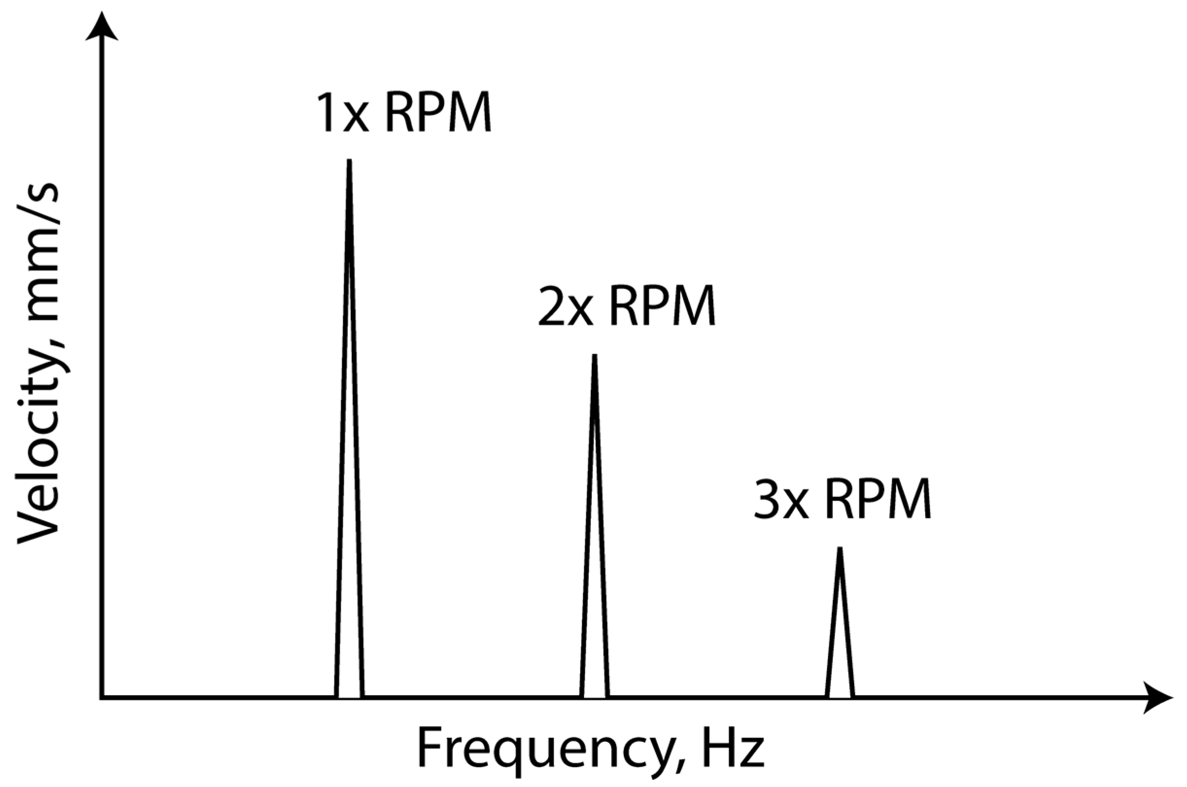
The velocity spectra in Figure 9a–d correspond to rotor faults and exhibit peaks at 1x, 2x, and 3x the rotating frequency. These harmonics indicate rotor defects, requiring expert analysis for diagnosis.

In contrast, Figure 9e lacks harmonic indicators of a bearing defect, typically occurring at higher frequencies. Thus, envelope analysis is applied to detect better-bearing faults. The vibrations are band-pass filtered from 2000–5000 Hz so that the filtered data contains the bearing-related vibration response. The Hilbert transform and the FFT analysis are performed on the envelope time-domain data to compute the envelope spectrum (Figure 10).

Figure 10a–d show no peaks, indicating no bearing faults present with the rotor faults. However, Figure 10e shows peaks at the 1x and 2x harmonics of the bearing cage frequency from Table 2, indicating a fault in bearing B2’s cage.

6. The VML Model

Sepulveda and Sinha [19] have used both time- and frequency-domain features to develop an ANN-based VML model to diagnose rotor-related faults. The study suggested six parameters (

Table 6. Parameters of vibration data in both the time and frequency domains [19].

Parameters	Domain	Amplitude
Root mean square (RMS)	Time	Acceleration
Kurtosis (K)	Time	Acceleration
The first harmonic of rotating speed (1x)	Frequency	Velocity
The second harmonic of rotating speed (2x)	Frequency	Velocity
The third harmonic of rotating speed (3x)	Frequency	Velocity
Spectrum energy (SE)	Frequency	Velocity

)—two in the time domain (acceleration RMS and kurtosis) and four in the frequency-domain parameters (1x, 2x, and 3x amplitudes of the velocity spectra and spectrum energy). These parameters were found to be robust parameters to detect rotor faults in the earlier study.

This study is also attempting to keep exactly the same ANN-based VML and the parameters to make this model as the standard VML model for both the rotor and anti-friction bearing fault detection. However, the following three essential modifications are implemented to include bearing-related vibration responses.

i.

The RMS values are calculated from the measured vibration data, which contain a frequency range up to 5000 Hz. Hence, the RMS values have rotor and bearing responses.

ii.

The bearing assembly and housing resonance frequency is likely to be in the band of 2000–5000 Hz for this bearing used in the rig. It is also known that the bearing defect frequencies (in the case of the bearing fault) are generally modulated around the bearing resonance frequency. Hence the kurtosis (FK) calculated on the band-pass filtered acceleration signals in the 2000 Hz to 5000 Hz frequency range so that kurtosis can reflect the bearing condition.

iii.

Similarly, like RMS, the frequency range for the spectrum energy (SE) calculation is expanded from 0.3 times the rotational speed to 5000 Hz. This adjustment accommodates the effects of subharmonics related to the rotor faults and the high band frequency range for the anti-friction bearing faults.

These time- and frequency-domain parameters are extracted from all measured vibration signals of the collected samples and all tested experimental conditions.

Table 7. Total data as the input for the ANN model.

Source of Data	Input Vector Size (No. of Parameters)	Measurement Points	Total of Samples	Training Samples (70%)	Validation Samples (15%)	Testing Samples (15%)
B1, B2, B3 and B4	24	4	240	168	36	36

provides the list of total data and the arrangement of their use within the ANN-based VML model.

The databank of the ANN’s input for each tested speed, Data, is constructed as follows:

$$Data={\left[\begin{array}{ccc}DataH& DataM& \begin{array}{cc}DataC& \begin{array}{cc}DataR& DataBF\end{array}\end{array}\end{array}\right]}^T$$

(9)

In this context, ‘$DataH$‘ refers to the databank for the healthy condition, ‘$DataM$’ corresponds to the databank for the misalignment fault condition, ‘DataC’ represents the databank for the cracked shaft fault condition, ‘$DataR$‘ is associated with the databank for the rotor rub fault condition, and ‘$DataBF$‘ denotes the databank for the bearing fault condition. Each of these databanks comprises parameters from individual runs. Each databank is arranged as per Equation (10).

$$\begin{gathered} DataH={\left[\begin{array}{ccc}{H}_1& H_2& \begin{array}{cc}\dots & H_{40}\end{array}\end{array}\right]}^T, \\ DataM={\left[\begin{array}{ccc}{M}_1& M_2& \begin{array}{cc}\dots & M_{40}\end{array}\end{array}\right]}^T, \\ DataC={\left[\begin{array}{ccc}{C}_1& C_2& \begin{array}{cc}\dots & C_{80}\end{array}\end{array}\right]}^T, \\ DataR={\left[\begin{array}{ccc}{R}_1& R_2& \begin{array}{cc}\dots & R_{40}\end{array}\end{array}\right]}^T, \\ DataBF={\left[\begin{array}{ccc}{BF}_1& {BF}_2& \begin{array}{cc}\dots & {BF}_{40}\end{array}\end{array}\right]}^T \end{gathered}$$

(10)

The subscripts 1, 2, 3, and so on denote the machine run or sample numbers, as detailed in Table 2. For the healthy machine condition, the parameters for each run, which consist of 24 elements (calculated as 6 parameters per bearing times 4 bearings), are organised according to the structure provided in Equation (11).

$$\begin{gathered} H_i=[ {RMS}_{{B1}_z} K_{{B1}_z} {1x}_z {2x}_{{B1}_z} {3x}_{{B1}_z}{ SE}_{{B1}_z}\dots \\ {RMS}_{{B2}_z}\dots {SE}_{{B2}_z} {RMS}_{{B2}_z}\dots {SE}_{{B3}_z} {RMS}_{{B4}_z}\dots {SE}_{{B4}_z}] \end{gathered}$$

(11)

where z is the healthy machine condition’s run number (sample number). Similarly, the databanks can be arranged for other machine fault conditions. Once the databanks are prepared, the VML model is applied, as discussed in Section 3.

7. Application of the ANN-Based VML Model and Results

The bearing fault is now included in the ANN-based VML used earlier [19]. The model in this study is designed to classify the state of the rotor and bearing system into five distinct conditions: healthy, misalignment, crack, rub, and bearing faults. Selected input parameters of the ANN are representative of the machine’s dynamic characteristics, including the RMS and FK of acceleration in the time domain, as well as the 1x, 2x, and 3x velocity spectra and the SE of velocity in the frequency domain. For a balanced learning process, we structured the dataset with 70% dedicated to training and the remaining 30% equally divided for validation and testing.

Upon developing the system at 900 RPM, the ANN-based VML model shows excellent performance, achieving 100% accuracy in identifying the healthy condition, rotor faults, and bearing faults (

Table 8. Overall performance of the VML model at a rotating speed of 900 RPM (above the first critical speed).

		Target Class
		Healthy	Misalignment	Crack	Rub	Faulty Bearing
Output Class	Healthy	100	0	0	0	0
	Misalignment	0	100	0	0	0
	Crack	0	0	100	0	0
	Rub	0	0	0	100	0
	Faulty Bearing	0	0	0	0	100

).

8. Further Validation

To ensure the reliability and applicability of the ANN-based VML model and the vibration parameters, the model is further tested at two other rotating speeds. These two speeds are 450 RPM (7.5 Hz), below the experimental rig’s first critical speed, and 1350 RPM (22.5 Hz), above the second critical speed. The input matrices are constructed using the same extracted parameters in both the time and frequency domains. The data arrangement process for the input matrixes is described in Section 6 and is followed in these exercises. The 100% correct identification of the machine conditions is observed, which is listed in

Table 9. Overall performance of the VML model at a rotating speed of 450 RPM (below the first critical speed).

		Target Class
		Healthy	Misalignment	Crack	Rub	Faulty Bearing
Output Class	Healthy	100	0	0	0	0
	Misalignment	0	100	0	0	0
	Crack	0	0	100	0	0
	Rub	0	0	0	100	0
	Faulty Bearing	0	0	0	0	100

and

Table 10. Overall performance of the VML model at a rotating speed of 1350 RPM (above the second critical speed).

		Target Class
		Healthy	Misalignment	Crack	Rub	Faulty Bearing
Output Class	Healthy	100	0	0	0	0
	Misalignment	0	100	0	0	0
	Crack	0	0	100	0	0
	Rub	0	0	0	100	0
	Faulty Bearing	0	0	0	0	100

. The rig dynamics are expected to be significantly different, but the VML model shows robustness. This is because the vibration parameters are selected based on the rotodynamic concept.

9. Concluding Remarks

The earlier ANN-based VML model and the optimised vibration parameters for only detecting rotor faults have now been extended to include both rotor and anti-friction bearing faults. The vibration parameters are revised by extending the frequency range up to 5000 Hz to cover the bearing-related resonance responses due to defects in the bearing. The proposed VML method is initially developed and applied to the experimental rig when rotating at 900 RPM (above the first critical speed). The model yields a 100% accurate diagnosis of the machine conditions. To further check the usefulness and robustness of the VML model and the vibration parameters, the proposed method is also tested on the same experimental rig but at two different speeds. These speeds are 450 RPM and 13,500 RPM, which are below the first critical speed and above the second critical speed, respectively. The machine dynamics are significantly different at these two speeds compared to the speed of 900 RPM. Still, the proposed vibration parameters and the ANN-based VML model gave a 100% correct diagnosis of the machine conditions. Hence, the model has the potential for industrial applications.

References

1. Muszynska, A. Rotordynamics; CRC Press: Boca Raton, FL, USA, 2005. [Google Scholar]
2. Perez, R.X. Rotating Machinery Repair Best Practices. Maint. Reliab. Troubl. Rotating Mach. 2022, 2, 205–226. [Google Scholar]
3. Liu, R.; Yang, B.; Zio, E.; Chen, X. Artificial intelligence for fault diagnosis of rotating machinery: A review. Mech. Syst. Signal Process. 2018, 108, 33–47. [Google Scholar] [CrossRef]
4. Almounajjed, A.; Sahoo, A.K.; Kumar, M.K.; Assaf, T. Fault diagnosis and investigation techniques for induction motor. Int. J. Ambient. Energy 2022, 43, 6341–6361. [Google Scholar] [CrossRef]
5. Yunusa-Kaltungo, A.; Cao, R. Towards developing an automated faults characterisation framework for rotating machines. Part 1: Rotor-related faults. Energies 2020, 13, 1394. [Google Scholar] [CrossRef]
6. Luwei, K.; Yunusa-Kaltungo, A. Data combination for a consolidated diagnosis of rotor and bearing faults. In Proceedings of the 12th International Conference on Vibrations in Rotating Machinery, Virtual, 14–15 October 2020; pp. 388–399. [Google Scholar]
7. Zhang, C.; Zhang, L. Wind turbine pitch bearing fault detection with Bayesian augmented temporal convolutional neural networks. Struct. Health Monit. 2023; ahead of print. [Google Scholar]
8. Jardine, A.K.; Lin, D.; Banjevic, D. A review on machinery diagnostics and prognostics implementing condition-based maintenance. Mech. Syst. Signal Process. 2006, 20, 1483–1510. [Google Scholar] [CrossRef]
9. Tama, B.A.; Vania, M.; Lee, S.; Lim, S. Recent advances in the application of deep learning for fault diagnosis of rotating machinery using vibration signals. Artif. Intell. Rev. 2023, 56, 4667–4709. [Google Scholar] [CrossRef]
10. Kumar, S.S.; Kumar, M.S. Condition monitoring of rotating machinery through vibration analysis. J. Sci. Ind. Res. (JSIR) 2014, 621, 1–9. [Google Scholar]
11. Tiboni, M.; Remino, C.; Bussola, R.; Amici, C. A review on vibration-based condition monitoring of rotating machinery. Appl. Sci. 2022, 12, 972. [Google Scholar] [CrossRef]
12. Yunusa-Kaltungo, A. Vibration-Based Condition Monitoring of Rotating Machines; The University of Manchester (United Kingdom): Manchester, UK, 2016. [Google Scholar]
13. Worden, K.; Staszewski, W.J.; Hensman, J.J. Natural computing for mechanical systems research: A tutorial overview. Mech. Syst. Signal Process. 2011, 25, 4–111. [Google Scholar] [CrossRef]
14. Chen, Z.; Deng, S.; Chen, X.; Li, C.; Sanchez, R.-V.; Qin, H. Deep neural networks-based rolling bearing fault diagnosis. Microelectron. Reliab. 2017, 75, 327–333. [Google Scholar] [CrossRef]
15. Mubaraali, L.; Kuppuswamy, N.; Muthukumar, R. Intelligent fault diagnosis in microprocessor systems for vibration analysis in roller bearings in whirlpool turbine generators real time processor applications. Microprocess. Microsyst. 2020, 76, 103079. [Google Scholar] [CrossRef]
16. Khoualdia, T.; Lakehal, A.; Chelli, Z.; Khoualdia, K.; Nessaib, K. Optimized multi layer perceptron artificial neural network based fault diagnosis of induction motor using vibration signals. Diagnostyka 2021, 22, 65–74. [Google Scholar]
17. Espinoza Sepúlveda, N.F.; Sinha, J.K. Blind application of developed smart vibration-based machine learning (SVML) model for machine faults diagnosis to different machine conditions. J. Vib. Eng. Technol. 2021, 9, 587–596. [Google Scholar] [CrossRef]
18. Mei, S.; Yuan, M.; Cui, J.; Dong, S.; Zhao, J. Machinery condition monitoring in the era of industry 4.0: A relative degree of contribution feature selection and deep residual network combined approach. Comput. Ind. Eng. 2022, 168, 108129. [Google Scholar] [CrossRef]
19. Sepulveda, N.E.; Sinha, J. Parameter optimisation in the vibration-based machine learning model for accurate and reliable faults diagnosis in rotating machines. Machines 2020, 8, 66. [Google Scholar] [CrossRef]
20. Igba, J.; Alemzadeh, K.; Durugbo, C.; Eiriksson, E.T. Analysing RMS and peak values of vibration signals for condition monitoring of wind turbine gearboxes. Renew. Energy 2016, 91, 90–106. [Google Scholar] [CrossRef]
21. Lei, Y.; Lin, J.; He, Z.; Zuo, M.J. A review on empirical mode decomposition in fault diagnosis of rotating machinery. Mech. Syst. Signal Process. 2013, 35, 108–126. [Google Scholar] [CrossRef]
22. McFadden, P.; Smith, J. Vibration monitoring of rolling element bearings by the high-frequency resonance technique—A review. Tribol. Int. 1984, 17, 3–10. [Google Scholar] [CrossRef]
23. Bracewell, R.N.; Bracewell, R.N. The Fourier Transform and its Applications; McGraw-Hill: New York, NY, USA, 1986; Volume 31999. [Google Scholar]
24. Randall, R.B. Vibration-Based Condition Monitoring: Industrial, Automotive and Aerospace Applications; John Wiley & Sons: Hoboken, NJ, USA, 2021. [Google Scholar]
25. Sinha, J.K. Industrial Approaches in Vibration-Based Condition Monitoring; CRC Press: Boca Raton, FL, USA, 2020. [Google Scholar]
26. Vyas, N.S.; Satishkumar, D. Artificial neural network design for fault identification in a rotor-bearing system. Mech. Mach. Theory 2001, 36, 157–175. [Google Scholar] [CrossRef]
27. Tarassenko, L. Guide to Neural Computing Applications; Elsevier: Amsterdam, The Netherlands, 1998. [Google Scholar]
28. Vogl, T.P.; Mangis, J.; Rigler, A.; Zink, W.; Alkon, D. Accelerating the convergence of the back-propagation method. Biol. Cybern. 1988, 59, 257–263. [Google Scholar] [CrossRef]
29. Bishop, C.M.; Nasrabadi, N.M. Pattern Recognition and Machine Learning; Springer: Berlin/Heidelberg, Germany, 2006; Volume 4. [Google Scholar]
30. Goodfellow, I.; Bengio, Y.; Courville, A. Deep Learning; MIT Press: Cambridge, MA, USA, 2016. [Google Scholar]
31. Ying, X. An overview of overfitting and its solutions. J. Phys. Conf. Ser. 2019, 1168, 022022. [Google Scholar] [CrossRef]
32. Luwei, K. Vibration-Based Fault Identification for Rotor and Ball Bearing in Rotating Machines. Ph.D. Thesis, University of Manchester, Manchester, UK, 2022. [Google Scholar]
Figure 1. An illustration of harmonics in the frequency-domain.
Machines 11 00943 g001
Figure 2. Actual sample of the velocity amplitude spectrum (V).
Machines 11 00943 g002
Figure 3. A schematic of a ball bearing.
Machines 11 00943 g003
Figure 4. A simple illustration of ball-bearing characteristic frequencies in the envelope spectrum.
Machines 11 00943 g004
Figure 5. Typical multi-layer perceptron (MLP) neural network of the study.
Machines 11 00943 g005
Figure 6. The laboratory-scaled rig setup.
Machines 11 00943 g006
Figure 7. A schematic drawing of the experimental rig.
Machines 11 00943 g007
Figure 8. Typical time−domain waveform at bearing 2 (B2) for the different machine faulty conditions at a rotating speed of 900 RPM. (a) Misalignment, (b) crack near B1, (c) crack near B2, (d) rub near D1, (e) faulty B2.
Machines 11 00943 g008
Figure 9. Typical velocity vibration spectra at bearing 2 (B2) for the different machine faulty conditions at a rotating speed of 900 RPM. (a) Misalignment, (b) crack near B1, (c) crack near B2, (d) rub near D1, (e) faulty B2.
Machines 11 00943 g009
Figure 10. Typical envelope spectra at bearing 2 (B2) for faulty machine conditions at a rotating speed of 900 RPM. (a) Misalignment, (b) crack near B1, (c) crack near B2, (d) rub near D1, (e) faulty B2.
Machines 11 00943 g010