Measuring Methods of Radius of Curvature and Tread Circle-Fitting Studies for Railway Wheel Profiles

Abstract

A railway wheel profile consists of short arcs with complex radii of curvature, and wheel wear leads to changes in the profile’s radius of curvature that ultimately affects the dynamic performance of the train. To track the evolution of in-service wheel profile curves, the radii of curvature of new foundry wheel profiles need to be measured. This study proposes a series of algorithms and calculation methods for measuring the radius of curvature of wheel profiles. Firstly, the curvature was estimated with the U-chord method, and the segment points were located. Secondly, the discrete derivative method and Two-Arcs Tangency Constrain (TATC) method were used to calculate the radius of curvature and the fitting circle radius, respectively. The experimental results of the three types of profiles showed that the wheel profile curves were precisely divided according to the estimated curvature method and that the maximum errors of the calculated results compared with standard values by the discrete derivative method and TATC method were 2.50% and 0.42%, respectively. Furthermore, the two measurement methods’ performances and repeated experiments were used to analyze the uncertainty.

1. Introduction

Rail transit is an important mode of transportation in industrialized countries. High-frequency and long-distance railway transportation has higher requirements for the safety and stability of trains. Due to the influence of external factors such as carrying capacity, rail terrain, rain erosion, and sudden braking, the situation of wheel wear inevitably occurs during long-term service [1]. The wheel profile is an important feature of the wheelset; hence, the timely detection of changes in the wheel profile is the main task of wheelset detection and maintenance. Research in wheel wear has been conducted by some scholars [2,3]; all of them have compared worn wheel profiles to standard ones and neglected errors between the fresh-from-factory forged wheels and standard wheels. Although these errors meet tolerance zone requirements, the manufacturing errors should be analyzed in deeper studies about of the principles of wheel wearing or wheel–rail contact. To conduct studies that explore the actual Hertzian or rolling contact parameters, it is important to measure the true parameters of newly forged wheels rather than using design criterion values directly.

Workers mainly use wheel vernier calipers or laser instruments to measure some horizontal and vertical parameters (i.e., flange height, flange width, rim width, QR), but these parameters cannot manifest changes in the whole wheel curve entirely. The most obvious change for integrated measurements is the radius of curvature. The design of the wheel profile shape is conducted based on many countries’ standards, and some additional factors must be considered, such as the degree of wheel-rail matching, vehicle stability, wearing model, and repair strategy. These reasons cause the wheel profile to have a complex curve shape with multiple arcs, as shown in Figure 1. These arcs’ radii of curvature influence the train dynamics; some researchers have studied this phenomenon and carried out design optimization research on wheel profile shapes [4,5]. Dynamic simulation experiments rely on the input of digital design curves, and the results of simulations present the wheel profile after wearing. When studying the mechanism of wheel wear, the Hertzian or rolling contact theory is often used; the parameters require the measurement of the radius of curvature at the contact point [6]. However, the actual wheel profile curve is not exactly consistent with the digital curve, and the curvature of the actual wheel profile curve needs to be detected at all wearing stages, especially from the initial wheel shape. In this way, wear experiments of the actual wheel and simulations can be compared more rigorously. This study laid emphasis on measuring the radius of curvature of a new (before serviced) wheel. This study enriches the original characteristics of wheel profiles and provides a reference for the future analysis of worn wheels.

The curvature estimation of curves is composed of sequentially sampling discrete points (hereafter referred to as discrete curves) and is commonly used in the field of differential geometry or digital image processing. Mokhtarian et al. [7] proposed the Curvature Scale Space (CSS) algorithm in 1998; the algorithm calculates the curvature based on the contours extracted from an image using the parametric arc length formula for a curve and then measures the degree of inflection response based on the curvature value of each pixel point. The CSS algorithm led to a series of improved algorithms, such as the Curvature Scale Space Corner with Adaptive Threshold (ATCSS) [8], Multi-scale Curvature Product (MSCP) [9], Direct Curvature Scale Space (DCSS) [10], and so on. Zhang et al. [11] employed Chebyshev polynomial fitting to estimate continuous curvatures in corner detection issues. Zhang et al. [12] proposed that variations in the evolution difference in contour curves at different scales could be taken as the corner response function, and the Difference of Gaussian (DoG) detection operator was proposed. Although these methods were based on digital image data, they defined a new curvature expression method to achieve the purpose of feature recognition. However, the true value of curvature was not calculated using these methods.

In the context of how to fit an arc of approximately circular points to an approximate circle, two categories can be divided from recent research [13]: (1) Geometric fitting: the objective is to minimize the orthogonal distance from the fitting circle in order to approximate circular points. (2) Algebraic fitting: the objective is achieved with a series of algebraic formulas. Unfortunately, all of these studies mentioned nothing about when the approximate circular points become short approximate circular arc points (i.e., the approximate circular points are inadequate compared with the whole circle), and the fitting results do not have position constraint requirements. Hu et al. [14] proposed a parameter-free approach for weighted geometric circle fitting, and the corresponding bias was investigated with the classical theory of nonlinear least squares in this study. Liu et al. [15] proposed a radius constraint method to measure the structured light arc of wear of a rail profile. Zhu et al. [16] proposed a center constraint method to measure a rotational workpiece. However, these methods required obtaining prior information about the radius or center of the circle coordinates. In actual on-site measurements, accurate prior information is hard to obtain for railway inspectors. Tao et al. [17] proposed a parameter-constrained fitting method based on a four-parameter circle equation, and the experimental results showed that this method had a high accuracy when measuring short arcs with small central angels without prior information.

In order to compare the evolution of a wheel profile curve before and after wearing, a newly forged wheel profile’s radii of curvature need to be measured. This research used a laser profile sensor to collect the wheel profile data. Aiming at the collected complex curve, a series of methods were proposed to measure the radius of curvature, which included demarcating segmented points (positioning tangency points), calculating the radius of curvature, and fitting a circle for small arcs. The remainder of this study consists of three parts. First, in Section 2, the theory of analysis and the calculation processing is proposed. The experimental device and profile data calculation are described in Section 3. In Section 4, the analysis of the uncertainty is summarized.

2. Radius of Curvature Determination of Wheel Profile

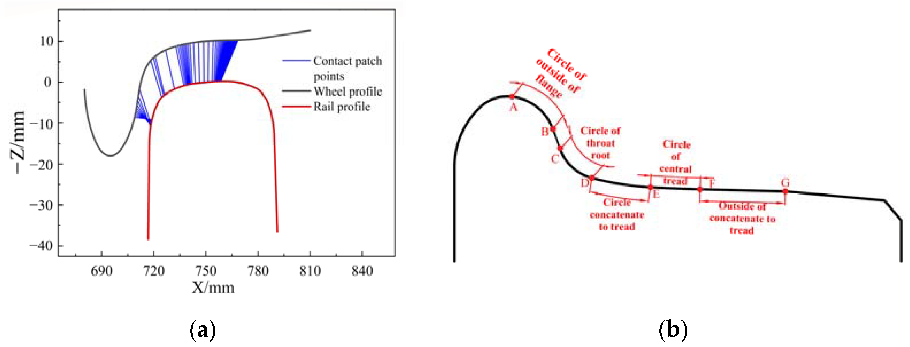
2.1. Composition of Wheel Profile Curve and Analysis Interests

During the function of train wheels, the wheel–rail contact point distribution is as shown in Figure 2 [18]. The wear of the wheel surface caused by wheel–rail contact mainly occurs in the circular arc AB, the linear section BC, the circular arc CD, the circular arc DE, the circular arc EF, and the linear section FG. There exist sudden changes in the curvature of the wheel profile at the segmented points, which adversely affect the contact point distribution [19]. Moreover, if the wheel profile curvature ρ_w is close to the rail profile curvature ρ_r, there exists a two-point contact or common contact, which aggravates wheel–rail wear [20,21]. Therefore, short arcs of the wheel profile curves and segmented points were selected as this study’s interests.

The following Figure 3 shows the methodology of the measuring procedure used to process the wheel profile curve.

2.2. Methods of Measuring the Radius of Curvature from the Discrete Curve of a Wheel Profile

The complex curve shape of a wheel profile can be measured by a laser profile sensor, as Figure 4 shows. The laser profile is based on the laser triangle principle [22], and the measured object’s profile is collected as a line point cloud, which is composed of a series of sample points with coordinates information. Thus, these sample points comprise a discrete curve of discrete point coordinates (x_n, y_n) [23,24,25].

2.2.1. U-Chord Curvature Estimation Method

For the task of wheel profile design, a curve line or a vector function expression of a curve with clear demarcation points can be constructed through computer-aided geometric design (CAGD) software. However, the wheel profile curves collected from on-site measurements contain noisy data points, and the demarcation point of the curve segment is not obvious in the visual field; therefore, it is first necessary to identify the segmented points (tangency points). Segmented points can be discovered by curvature estimation. This research used the U-chord curvature method to estimate the segmented point positions of each short arc and used a refined curve strategy according to the difference between the curve of the discrete points and the digital curve.

The method begins with the following:

$$l=\left\{P_i|\left(x_i,y_i\right),i=1,2,\dots n\right\}$$

(1)

$$\mathsf{\Omega }\left(P_i\right)=\left[P_{i-b}, P_{i+f}\right]$$

(2)

$$\left|P_i{P}_{i-b}\right|=\left|P_i{P}_{i+f}\right|=\mathrm{U}$$

(3)

From Equations (1) and (2), l is defined as a discrete point curve, and Ω is the constraint-supported domain, which is determined by selected parameter U. The parameter U is subjected to the constraint condition, as shown in Equation (3). Since no point of the discrete curve absolutely satisfies Equation (3), the points $P_{i-b}$ and $P_{i+f}$ that satisfy the support domain are searched by the following algorithm (Algorithm 1), and the theory is shown in Figure 5.

Algorithm 1. U-chord curvature method of discrete curve.
Input:	U: the constraint-supported domain.
	Pi (xi, yi): points’ coordinates of the discrete curve.
	imax: the maximum number of points in one discrete curve.
Output:	Ui: the estimated curvature value of each point in the profile curve.
	$U_i=s_i\sqrt{1-{\left(\frac{D_i}{2U}\right)}^2}$	(4)
	$s_i=sign\left[\left(x_i-x_{i-b}\right)\left(y_{i+f}-y_{i-b}\right)-\left(x_{i+f}-x_{i-b}\right)\left(y_i-y_{i-b}\right)\right]$	(5)
	$D_i=\Vert P_{i-b}{P}_{i+f}\Vert$	(6)

According to the calculated results of the U_i distribution of each point, the segmented point of the wheel profile curve is determined. The coordinates of the segmented points of the profile wheel are determined according to the locations of the U_i curve saltation points.

2.2.2. Discrete Derivative Method Analysis for Wheel Profile Discrete Curve

Generally speaking, the connection between the derivative and the radius of curvature results in ways to calculate the radius of curvature. However, the wheel profile curve is discrete, and the function is not written directly. The solution of the discrete derivatives method [26] is based on differential geometry and tangent line estimation. The tangent line l of the point P_k (x_k, y_k) is set, whose discrete point function is y_i = f(x_i) (i∈{1, 2, …, n}), and the tangent line l has two attributes: (1) the tangent line passes through a fixed point P_k; and (2) the tangent line is a local line approximation of the fixed point’s symmetric neighborhood domain. In other words, the sum of the perpendicular distances from the points from the P_k symmetric neighborhood domain to the tangent line is a minimum. According to the above attributes, the relationship between tangent line l and y_i = f(x_i) based on the least squares method can be described as follows:

$$\mathit{min}f\left(a,b\right)={{\displaystyle \sum }}_{j=k-m}^{k+m}{\left(y_j-a{x}_j-b\right)}^2,\mathrm{s}.\mathrm{t}.{\tilde{\mathrm{y}}}_k=a{x}_k+b$$

(7)

The Lagrange multiplier is used to construct the Lagrange function:

$$L\left(a,b,\lambda \right)={{\displaystyle \sum }}_{k-m}^{k+m}{\left(y_j-a{x}_j-b\right)}^2+\lambda \left({\tilde{\mathrm{y}}}_k=a{x}_k+b\right)$$

(8)

When setting $\frac{\partial L}{\partial a}=0,\frac{\partial L}{\partial b}=0,\frac{\partial L}{\partial \lambda }=0$, the result is as follows:

$$a=f^{\prime }\left(\mathrm{x}\right)=\frac{{{\displaystyle \sum }}_{j=k-m_1}^{k+m_1}\left(x_j-x_k\right)\left(y_j-y_k\right)}{{{\displaystyle \sum }}_{j=k-m_1}^{k+m_1}{\left(x_j-x_k\right)}^2}$$

(9)

The differential result value $f^{\prime }\left(x_k\right)$ of point P_k is replaced by the curvature value a, and m₁ is the value of half of the neighborhood domain’s distance calculated from the point P_k. Furthermore, the differential coefficient result value $f^{″}\left(x_k\right)$ can be calculated by $f^{\prime }\left(x_k\right)$; similarly to Equation (9), the second derivative value of point P_k is calculated with Equation (10).

$$f^{″}\left(\mathrm{x}\right)=\frac{{{\displaystyle \sum }}_{j=k-m_2}^{k+m_2}\left(x_j-x_k\right)\left({y^{\prime }}_j-{y^{\prime }}_k\right)}{{{\displaystyle \sum }}_{j=k-m_2}^{k+m_2}{\left(x_j-x_k\right)}^2}$$

(10)

Due to the correlation between the numerical value of the radius of curvature and the derivative value, the radius of the curvature value is calculated with Equation (11).

$$k=\frac{1}{r}=\frac{\left|f^{″}\left(x\right)\right|}{{\left(1+f^{″}{\left(x\right)}^2\right)}^{\frac{3}{2}}}$$

(11)

In spatial analytic geometry, space curves are represented by parameterization, i.e., the coordinates of a point p on the space curve are written as a scalar function of a parameter u, as shown in Equation (12). In differential geometry, these forms are written as row vectors; thus, the normal curve is represented as a vector function about parameter u, as shown in Equation (13).

$$x=x\left(u\right),y=y\left(u\right),z=z\left(u\right)$$

(12)

$$p_i={\alpha }_d\left(u_i\right)=\left(x_d\left(u_i\right),y_d\left(u_i\right)\right),u_i\in \left\{u_{1,}{u}_{2,\cdots ,}{u}_n\right\}$$

(13)

In Equation (13), due to the wheel profile in two-dimensional space, only the x and y coordinates are parameterized. In contrast to the normal continuous differentiable parametrized curve, the wheel profile curve is discrete. The purpose of parameterization is to assign corresponding parameters to the curve points and, in turn, build an approximate function expression to approach the discrete curve. The common parameterization methods include uniform, cumulative chord length, endocentric parameters, Foley, and so on. In this research, the cumulative chord length method was selected to assign parameter u, and the u_i of each point P_i(x_i, y_i) was calculated as shown in Equation (14).

$$\left\{\begin{array}{c}{u}_1=0\\ u_i={\displaystyle \sum }_{j=1}^{i-1}\Vert p_{j+1}-p_j\Vert /{\displaystyle \sum }_{j=1}^{n-1}\Vert p_{j+1}-p_j\Vert ;i=2,3,\dots ,n;j=1,2,\dots ,i-1\end{array}\right.$$

(14)

The wheel profile curve can be written as follows:

$${\alpha }_d^{\prime }\left(u_i\right)=(x_d^{\prime }\left(u_i\right),y_d^{\prime }\left(u_i\right)$$

(15)

According to the definition of partial derivatives and discrete differentials, the specific first derivative is shown in Equation (16), and the second derivative has a similar form.

$$\left\{\begin{array}{c}{x}_d^{\prime }\left(u_i\right)=\frac{{{\displaystyle \sum }}_{j=i-m_1}^{i+m_1}\left(u_j-u_i\right)\ast \left(x_j-x_i\right)}{{{\displaystyle \sum }}_{j=i-m_1}^{i+m_1}{\left(u_j-u_i\right)}^2}\\ y_d^{\prime }\left(u_i\right)=\frac{{{\displaystyle \sum }}_{j=i-m_1}^{i+m_1}\left(u_j-u_i\right)\ast \left(y_j-y_i\right)}{{{\displaystyle \sum }}_{j=i-m_1}^{i+m_1}{\left(u_j-u_i\right)}^2}\end{array}\right.$$

(16)

Naturally, the radius of curvature value of Equation (11) can be re-written as follows:

$$\mathrm{r}=\frac{1}{k}=\frac{{\left(x_d^{\prime }{\left(u_i\right)}^2+y_d^{\prime }{\left(u_i\right)}^2\right)}^{\frac{3}{2}}}{\left|x_d^{″}\left(u_i\right)\ast y_d^{\prime }\left(u_i\right)-y_d^{″}\left(u_i\right)\ast x_d^{\prime }\left(u_i\right)\right|}$$

(17)

2.2.3. The Circle-Fitting Method of TATC

The sectors of a connection tread circle and central tread circle captured from a wheel profile have flat and large curvature values. Moreover, these two arcs comprise a large proportion of the whole profile curve; thus, the quantity of noise points (outliers) caused by uneven light reflection or overexposure is greater than those for other arcs. The discrete derivative method is defined in the local neighborhood approximation domain, and if a set of noise points are mixed in the neighborhood domain, the calculation result is widely affected. Therefore, the fitting circle method is applied in the circle of the connection tread and the circle of the central tread, as well as according to the result of the circle fitting in order to estimate the radius of the osculating fitting circle.

A wheel profile consists of continuous short arcs, that is, there exists a tangency relation between every two arcs. The circle of connection tread and the circle of the central tread are no exception. In this study, we proposed a two-arcs tangency constraint (hereinafter referred as to TATC) method to fit a circle via a new objective function. The basic idea of TATC is to fix a circle and establish another circle that fits the objective function. Then, the LM (Levenberg–Marquardt) algorithm and IRLS (iteratively reweighted least squares) method were used to solve the objective function. Since the radius value of the former circle is included in the latter circle’s parameters, the tangency relationship can be guaranteed. This study selected the circular arc of DE as the fixed circle O₂, using the TATC method in detail as follows.

The set of points from the circular arc of EF were defined as P¹_i (x¹_i, y¹_i) according to the mathematical formula of a circle ${\left(x-A\right)}^2-{\left(y-B\right)}^2=R^2$, establishing the fitting circle objective function of EF:

$$f=\mathit{min}{{\displaystyle \sum }}_{i=1}^n{\left(x_i^1-a_1\right)}^2+{\left(y_i^1-b_1\right)}^2-R_1^2$$

(18)

In Equation (18), (a₁, b₁) is the center coordinate of fitting circle O₁, n is the number of points from the arc of EF, and R₁ is the radius of fitting circle O₁. On account of the tangency relation there exists the following relationship between circles O₁ and O₂:

$$\sqrt{{\left(a_1-a_2\right)}^2-{\left(b_1-b_2\right)}^2}=R_1-R_2$$

(19)

In Equation (19), (a₂, b₂) is the center coordinate of fitting circle O₂, and R₂ is the radius of fitting circle O₂, which requires R₁ > R₂. a₂, b₂, and R₂ could be obtained from previous studies [27]. Equation (19) is substituted into Equation (18), and the objective function is changed, as the following shows:

$$f=\min {{\displaystyle \sum }}_i^n\rho \left({\epsilon }_i\right)$$

(20)

$${\epsilon }_i=\sqrt{{\left(x_i^1-a_1\right)}^2+{\left(y_i^1-b_1\right)}^2}-\left(\sqrt{{\left(a_1-a_2\right)}^2-{\left(b_1-b_2\right)}^2}+R_1\right)$$

(21)

In Equations (20) and (21), ε_i is the error of fitting precision, $\rho \left(·\right)$ represents the loss function, and Cauchy’s function [28] was chosen to construct the loss function in this study, as shown in Equation (22). Equation (23) is the derivation result of Equation (22), and Equation (23) was used to calculate the Jacobian matrix of the objective function. Equation (24) is the ratio of Equation (23)/Equation (21) and is a defined weight function.

$$\rho \left({\epsilon }_i\right)=\frac{{\epsilon }_i^2}{2\ast \ln \left(1+{\left(\frac{{\epsilon }_i}{\sigma }\right)}^2\right)}$$

(22)

$$\psi {\epsilon }_i=\frac{{\epsilon }_i}{\left(1+{\left(\frac{{\epsilon }_i}{\sigma }\right)}^2\right)}$$

(23)

$$w_c{\epsilon }_i=\frac{1}{\left(1+{\left(\frac{{\epsilon }_i}{\sigma }\right)}^2\right)}$$

(24)

$$f=argmin{{\displaystyle \sum }}_{i=1}^n\Vert w_c\left({\epsilon }_{i,k-1}\right)\ast \rho \left({\epsilon }_i\right)\Vert$$

(25)

In the equations, σ is a variable of scale parameter, and the variable is updated by Equations (26)–(28). ${\epsilon }_{i,k-1}$ represents the fitting error value, which is calculated by inputting k−1th times the fitting circle results into the calculation at point P_i.

$$\frac{1}{1+{\left[\frac{M\left({\epsilon }_{i,0}\right)}{{\sigma }_0}\right]}^2}=0.8$$

(26)

$${\sigma }_k=\left\{\begin{array}{cc}\hfill {\sigma }_0,& k=0\hfill \\ \hfill \frac{\xi \ast {\sigma }_{k-1}}{\ln \left(e+n_s\right)+\tau },& k\ne 0\hfill \end{array}\right.$$

(27)

$$\frac{1}{1+{\left(\frac{\delta }{\tau }\right)}^2}=0.8$$

(28)

In Equation (26), M (·) is the median function, and ${\epsilon }_{i,0}$ is the fitting error value of the first iterative calculation. σ₀ is the scale parameter of the first iterative calculation, where the value of σ₀ is determined by Equation (26), and the latter value is determined by Equation (27). In Equation (27), ξ is a convergent parameter, and e is the natural logarithm. $n_s$ is the number of iterations. τ is an accelerated parameter of convergence, as shown in Equation (28). In Equation (28), δ is the noise intensity value of measurement, and it is determined by the sensor’s precision. Through Equations (26)–(28), the value of σ in Equations (22)–(24) is decided.

The nonlinear objective function, as shown in Equation (25), is difficult to solve with the least squares method. Common solution methods include the Gauss–Newton iteration method and the gradient descent method. The Gauss–Newton method is sensitive to the initial values, which is in contrast to the gradient descent method. Therefore, in order to preserve solution procedure accuracy, the LM (Levenberg–Marquardt) algorithm was chosen in this research, and is written concretely as follows:

$$\left[J_f^T{J}_f+\mu I\right]h=-J_f^{T}f$$

(29)

In Equation (29), μ is the damping coefficient, h is the direction of iteration, J is the Jacobian matrix of the objective function, I is the identity matrix, and f is the objective function. The trust region method was applied in the LM algorithm, which can update the damping coefficient μ. Next, in order to reduce the influence of noise points when calculating a fitting circle, the idea of IRLS was introduced: when the kth calculation is completed, the calculation results (i.e., the coordinate of the center of circle O₁ (a₁^k−1, b₁^k−1)) of k times are input into Equation (23); each point’s error (i.e., ${\epsilon }_{i,k-1}$) in arc EF is calculated. Then, Equations (24)–(29) are utilized to update the objective function Equation (25). Then, the objective function is solved using Equation (29) again.

The detailed algorithm is as follows (Algorithm 2):

Algorithm 2. Two-Arcs Tangency Constraint (TATC) method
Input:	P1i (x1i, y1i): data points of arc EF.
	P2i (x2i, y2i): data points of arc DE.
	[a2, b2, r2]: circle O2 parameters [27].
	w0: initial weight matrix.
	qmax: the maximum number of iteration times.
	Δq: the minimum precision.
Output:	[a1, b1, r1]: circle O1 parameters.

3. Experimental Testing and Analysis

3.1. Experimental Equipment and Test Objectives

A laser profile sensor was used to scan the wheel profile, and the sensor equipment and measurement procedure are shown in Figure 6. The detailed key performance parameters of the sensor are shown in

Table 1. The key performance parameters of the laser sensor.

Parameters	Value
Maximum sample points in one line point cloud	1920
Repeatability of x-axis	40 μm
Repeatability of z-axis	20 μm
Linearity	±0.01 %FS
Temperature drift	±0.01 %FS·°C−1

. The three types of scanned wheel profiles included LM_A, LM_C, and JM, all of which are common types of wheels in service train bogies, and the standard values of each profile are shown in

Table 2. The segmented parameters of different wheel profile types.

Wheel Profile Type	Radius of Outside of Flange Circle (arc AB)/mm	Radius of Throat Root Circle (arc CD)/mm	Radius of Connection Tread Circle (arc DE)/mm	Radius of Central Circle (arc EF)/mm	Outside of Connection to Tread
LMA	15	14	90	450	1:40
LMC	25.05	13	The curve of a set of points		5.5:100
JM	20	14	100	500	R200

[29].

3.2. Segmentation Point Experiments Based on U-Chord Curvature Estimation

The wheel profile collected by the sensor is shown in Figure 7. The LM_A-type profile had 1588 points, and the LM_C- and JM-type profiles had 1540 and 1539 points, respectively. Thus, the three types of wheel profiles had similar shapes but different radius curvature arcs, as Table 2 shows.

When inputting the discrete curve of the wheel profile, Algorithm 1 was chosen to estimate the U-chord curvature method. Then, the segmented points’ coordinates of each arc were determined. The U-chord curvature method’s result was affected by input parameter U; thus, inputting different parameters and comparing the results was used to find the best distinct curvature distribution. Taking the LM_A-type profile as an example, the results are shown in Figure 8.

Figure 8a–f represent the U-chord curvature results from selecting different values of U (i.e., U = 1.2, …, 2.2.); in each parameter case, the curvature of each point was estimated, and the wheel profile curve was drawn on the same sheet, which facilitated the observation of the curvature distribution of each point on the profile curve. In fact, the U-chord curvature method is also a class of curvature scale space, and different U values present different parameters of scale space. It is necessary to find the most distinctive features in a scale space. The demarcation points of each segment arcs can be determined by the local peak point or bottom point. In Figure 8a–c, the wave of the estimated curvature was too disordered. In Figure 8e, point E and point F were not clearly recognized. In Figure 8d, when the value of U was equal to 1.8, the segmented points A~F were distinguishable, and the segmented points were marked by recognition.

In order to verify the accuracy of the segmented point coordinates, a collected curve of a wheel profile was registered to the wheel profile of the Chinese national standard [29,30], as shown in Figure 9. According to the corresponding points of the two different source curves, the selected segmented points’ indexes and coordinates from the scanned curve were compared to position accuracy.

Figure 9 shows the coordinate transformation results of the scanned LM_A-type profile, which were registered to standard values plotted by the CAD software. The points’ indexes were recorded before and after registration, as shown in

Table 3. Comparison of the estimated and the standard segmented points’ coordinates according to registration.

Segmented Points	Index	Coordinates after Registration/mm	Coordinates of Standard/mm	Errors/mm
A	155	(−55.629, 27.834)	(−55.557, 27.913)	0.106
B	448	(−40.305, 17.980)	(−40.265, 18.152)	0.278
C	492	(−38.089, 11.849)	(−38.026, 12.295)	0.450
D	663	(−28.076, 3.244)	(−28.471, 3.327)	0.474
E	953	(−10.245, 0.473)	(−10.750, 0.499)	0.506
F	1206	(4.492, −0.163)	(4.254, −0.127)	0.790

. The maximum error was 0.790 mm; thus, the selected points could be thought of as arc demarcation points.

3.3. The Radius of Curvature Calculation Based on Discrete Derivative Method

According to the results of Section 2.2, we adopted the discrete derivative method to calculate the radius of curvature of the wheel profile. The discrete derivative needs to determine the value of the neighborhood domain m₁, m₂. Hence, a pre-experiment was performed before the formal experiment, whose purpose was to select a suitable neighborhood domain to adapt different curvatures.

The wheel profile curve was divided into two classifications due to the morphology of the curve, as shown in Figure 10. On the basis of the wheel profile types in service from China’s national standard, the value of the radius of curvature of the convex arcs included 15, 16, 18 mm, and so on; the radius of the concave arcs included 13 and 14 mm. Thus, a radius calibration block was used in the pre-experimentation, and a suitable neighborhood domain value was determined. The pre-experiment process is shown in Figure 11.

According to the results of the pre-experiment, and combined with the segmented points, the results of the discrete derivative experiment are shown in Figure 12; each segment arc’s radii of curvature values are shown in

Table 4. The results of calculating LM_A-type profile’s radius of curvature.

Segments	Standard Value of the Radius of Curvature/mm	DD Method/mm	Huang Method/mm	Yang Method/mm
The left side of point A	12	12.210	16.357	14.796
AB	15	15.274	18.844	18.248
CD	14	14.307	17.397	17.781
DE	90	119.038	131.042	121.004
EF	450	251.714	230.625	247.846

,

Table 5. The results of calculating LM_c-type profile’s radius of curvature.

Segments	Standard Value of the Radius of Curvature/mm	DD Method/mm	Huang Method/mm	Yang Method/mm
The left side of point A	12	12.336	16.127	16.819
AB	25.05	24.586	21.091	27.334
CD	13	13.325	17.751	16.764

and

Table 6. The results of calculating JM-type profile’s radius of curvature.

Segments	Standard Value of the Radius of Curvature/mm	DD Method/mm	Huang Method/mm	Yang Method/mm
The left side of point A	12	12.430	14.893	14.971
AB	20	19.881	24.295	22.501
CD	14	14.311	16.348	15.084
DE	100	131.746	152.082	144.659
EF	500	449.522	421.574	312.472

. The Huang method [31] and the Yang method [32] were selected for comparison. In the figures and tables, the discrete derivatives are written as DD; the different methods’ relative errors are plotted in Figure 13.

As shown in Figure 12, to the left side of point D, or in other words, in the small radius of curvature segments, the discrete derivative method had high-precision results. According to Table 4, the relative error was less than 3.05%. The Huang and Yang methods are based on calculating the tangency circle in the radius curvature definition; however, these methods had large errors in their high-density line point cloud data. In the arcs of DE and EF, with the increase in the radius of curvature, the noise points caused by the laser source had a great effect on the calculation results, and the discrete derivative method was no longer applicable. The same situation was observed in the measurements of the other two profiles.

As shown in Table 5 and Table 6, similar situations also occurred in the LM_C- and JM-type wheel profiles. All of the results in the small-radius curvatures had a high accuracy, and the maximum relative errors in the two types were less than 3.23% and 3.58%, respectively. Furthermore, both the DE and EF arcs’ measurement errors severely deviated. The test environment and the associated definition of the discrete derivative, as well as the existence of noise data points, contributed to the approximate calculation errors. Moreover, the noise points affected the symmetric neighborhood domain, and a tiny change in the neighborhood domain influenced the calculation results.

3.4. The Fitting Circle Experiment of the Circle of the Connection Tread and the Circle of the Central Tread

Using the Pratt fitting circle method to fit the data points from arc DE, the fitting result of the radius was 90.3969 mm, and the relative error of the standard value was 0.44%. According to Algorithm 2, the fitting circle result of arc EF was calculated, as shown in Figure 14. The result of the Pratt method used to fit the points of arc EF was 481.869 mm; this gave a large discrepancy compared with the standard value. This was because arc EF had noise data. The arc was short and had a small central angle, making the circle shape sensitive to noise points. The fitting result was unsatisfactory, and the noise data are shown in Figure 15.

The TATC method considered the link of the parameters of arc DE when fitting the circle to arc EF, and the result was 451.820 mm, and the relative error was 0.40%. This was because the TATC method’s objective function was based on the tangency relation of arc DE, and the radius was constrained by arc DE’s parameters. In addition, the distance of the two circles’ tangency point to the segmented point E was 0.719 mm; this result showed that the tangency relation was met from another point of view.

In addition, the wheel profile of the JM type was also tested. The general result of fitting the circle of arc EF is shown in Figure 16a. Similarly to the calculating process of the LM_A-type curve, the Pratt fitting result of arc DE’s radius was 100.512 mm, and the arc EF was 470.451 mm. The local results of the TATC method are shown in Figure 16b–d. The radius of curvature value calculated by the TATC method was 492.461 mm, and the relative error was 1.51%. It was found that the cambered curve position of fitting the circle by the TATC method was closer to the standard circle than that of the Pratt method, as shown in Figure 16b,c, and the value showed a high precision. Figure 16d shows the noise points of the scanned curve segments, and the Pratt method was effectively influenced by these undulating points. The IRLS method, which was used in the TATC calculating process, played a role in facing noise points. Despite the Pratt method fully taking into consideration the minimization of the fitting errors, the noise points’ influence affected the measurement accuracy. Thus, the procedure of reweighting with Equation (24) was necessary.

4. The Measurement Analysis of Uncertainty Evaluation

As a result of the existence of measuring errors and calculation errors, the true value was difficult to obtain. Generally, the uncertainty of measurement is used to reflect the quality and credibility of the determined values. Through a discrete derivative method and the TATC method, the LM_A type was used as an example, and arc AB and arc EF were selected as the objects of the study.

In the following chapters, we kept four decimal places during the display of the calculated processing (the data figures collected by the laser profile sensor were in units of microns). In the final results, we consulted the relevant regulations of significant figures and the round-off method, and we kept two significant figures in the uncertainty values to ensure that the decimal point had the same placeholder of digits.

4.1. The Uncertainty Analysis in arc AB

4.1.1. Type-A Standard Uncertainty of arc AB

Table 7. Three sets of wheel profile curve measuring results.

Radius of Curvature/mm	Arc AB	Arc EF	Arc AB	Arc EF	Arc AB	Arc EF
Position	Set 1		Set 2		Set 3
1	15.271	452.088	15.213	451.701	15.271	451.751
2	14.956	452.518	14.896	452.582	15.026	452.677
3	15.021	451.914	14.953	452.218	14.936	451.751
4	14.952	451.913	15.044	452.506	15.103	452.441
5	15.038	452.629	15.128	452.551	15.092	452.462
6	15.175	449.924	15.073	449.372	15.126	449.214
7	15.215	449.534	15.151	450.063	15.174	449.160
8	15.041	448.036	15.034	447.981	15.085	447.831
9	15.194	449.075	15.208	449.057	15.172	449.061
10	15.109	451.980	15.121	452.399	15.125	451.895

shows three sets of experiments; every set was scanned at different times (different environmental sunlight), different temperatures, and different operators, but all of them were in the same ten positions of the train wheel profile. Bayes information fusion, which is based on both prior information and present sample information, was selected to analyze the results of the wheel profile radius of curvature [33].

$${\mu }_1=\mathrm{E}\left[h(\mu |x)\right]=\frac{{\mu }_0\ast {\tau }_1^2+n\ast {\sigma }_0^2\ast \overline{x_1}}{n\ast {\sigma }_0^2+{\tau }_1^2}$$

(30)

$${\sigma }_1=\sqrt{D[h(\mu |x)]}=\sqrt{\frac{{\tau }_1^2\ast {\sigma }_0^2}{n{\ast \sigma }_0^2+{\tau }_1^2}}$$

(31)

Figure 17 shows the calculation procedure for arc AB. Hence, the best estimated value of the radius of curvature from the three sets was 15.0984 mm, and the type-A standard uncertainty $u_a$ was 0.0211 mm. The degrees of freedom in the type-A evaluation of measurement uncertainty was equal to the degrees of freedom of the standard deviation, i.e., $3\ast \left(10-1\right)=27$.

4.1.2. Type-B Uncertainty of arc AB

According to Table 1, the precision parameters of the laser sensor included linearity and repeatability. In the case of arc AB, the accuracy of the uncertainty results of the radius of curvature largely depended on the ordinate axes of the area of the arc, i.e., the sag across the arc. For these purposes, the arch height and chord length of arc AB were considered in the uncertainty analysis, and the uncertainty model was as follows:

As shown in Figure 18, the relationship of the radius and the straight-line distance parameters (arch height h and chord length S) is shown in Equation (32).

$$R\approx \frac{S^2}{8h}+\frac{h}{2}$$

(32)

The sensitivity coefficients were calculated as follows:

$$C_s=\frac{\partial R}{\partial S}=\frac{S}{4h}$$

(33)

$$C_h=\frac{\partial R}{\partial h}=-\frac{S^2}{8h^2}+\frac{1}{2}$$

(34)

The actual measurement results showed that the values of S and h were 15.3247 mm and 3.0820 mm, respectively.

Table 8. The procedure budget about the uncertainty of arc AB.

Component of Uncertainty	Symbol	Calculation	Confidence Coefficient	Value/mm
Type-A standard uncertainty	$u_a$	Equations (30) and (31)	——	0.0211
Repeatability and linearity of x-axis direction	$u_{bS1}$	$u_{bS1}=0.04+S\times 0.01\%$	$\sqrt{3}$	0.0240
Temperature drift of x-axis direction	$u_{bS2}$	$u_{bS2}=15\times S\times 0.01\%$	$\sqrt{3}$	0.0133
Type-B uncertainty about x-axis direction component	$u_{bS}$	$u_{bS}=\sqrt{{\left(u_{bS1}\right)}^2+{\left(u_{bS2}\right)}^2}$	——	0.0274
Repeatability and linearity of z-axis direction	$u_{bh1}$	$u_{bh1}=0.02+h\times 0.01\%$	$\sqrt{3}$	0.0117
Temperature drift of z-axis direction	$u_{bh2}$	$u_{bh2}=15\times h\times 0.01\%$	$\sqrt{3}$	0.0018
Type-B uncertainty about z-axis direction component	$u_{bh}$	$u_{bh}=\sqrt{{\left(u_{bh1}\right)}^2+{\left(u_{bh2}\right)}^2}$	——	0.0118
Type-A standard uncertainty	$u_b$	$u_b=\sqrt{{\left(C_S\ast u_{bS}\right)}^2+{\left(C_h\ast u_{bh}\right)}^2}$	——	0.0896
The combine standard uncertainty	$u_c$	$u_c=\sqrt{{\left(u_a\right)}^2+{\left(u_b\right)}^2}$	——	0.0920

shows the budget of calculating the uncertainty of arc AB. The degrees of freedom of the type-B evaluation of measurement uncertainty were calculated with the following equation:

$$v_i\approx \frac{1}{2}\frac{u^2\left(x_i\right)}{{\sigma }^2\left[u\left(x_i\right)\right]}\approx \frac{1}{2}{\left[\frac{\mathrm{\Delta }u\left(x_i\right)}{u\left(x_i\right)}\right]}^{-2}$$

(35)

The actual calculation results showed that $\mathrm{\Delta }u\left(x_i\right)/u\left(x_i\right)\approx 0$ and that the value of $v_i$ was too large. This meant that the probability of the measured value falling outside the interval was low. Finally, the coefficient value k was 1.96 when setting the confidence interval as 95%. Consequently, the expand uncertainty $U=k\ast u_c\approx 0.1803$ mm.

4.2. The Uncertainty Analysis in arc EF

4.2.1. Type-A Uncertainty Analysis of arc EF

Similarly, aiming to assess arc EF by means of using Equations (30) and (31), the best estimated value of the radius of curvature from the three sets was 450.8590 mm, and the type-A standard uncertainty $u_{\mathrm{a}}$ was 1.0945 mm. In the same way, the degrees of freedom in the type-A evaluation of measurement uncertainty was equal to the degrees of freedom of standard deviation, i.e., $3\ast \left(10-1\right)=27$.

4.2.2. Type-B Uncertainty Analysis of arc EF

There was a difference with arc AB, because the arc of EF was measured by the fitting circle method; the computational solution function can be expressed approximately as a least squares model:

$$\mathrm{R}=\frac{1}{M}{{\displaystyle \sum }}_{k=1}^M\sqrt{{\left(x_k-X_0\right)}^2-{\left(y_k-Y_0\right)}^2}$$

(36)

In Equation (36), ($x_k$, $y_k$) is the coordinate point of fitting points, and M is the number of points. R is the value of the fitting circle’s radius. According to Equation (37), the value of the radius is affected by every point in the arc curve, and the errors of those points are measured independently. Thus, the type-B standard uncertainty $u_{\mathrm{B}}$ was calculated as follows:

$$u_b=\sqrt{{{\displaystyle \sum }}_{i=1}^M{\left(C_{x_i}{u}_{x_i}\right)}^2+{{\displaystyle \sum }}_{k=1}^M{\left(C_{y_i}{u}_{y_i}\right)}^2}$$

(37)

In Equation (37), $u_{x_i}$ and $u_{y_i}$ are the errors of the x-axis and z-axis, respectively. $C_{x_i}$ and $C_{y_i}$ are sensitivity coefficients, which can be calculated by taking Equation (37) to the partial derivatives of $x_k$ and $y_k$.

$$C_{x_i}=\frac{\partial R}{\partial x_i}=\frac{1}{M}\frac{x_i-X_0}{\sqrt{{\left(x_i-X\right)}^2-{\left(y_i-X\right)}^2}}$$

(38)

$$C_{y_i}=\frac{\partial R}{\partial y_i}=\frac{1}{M}\frac{y_i-Y_o}{\sqrt{{\left(x_i-X\right)}^2-{\left(y_i-X\right)}^2}}$$

(39)

The detailed calculation parameters are shown in

Table 9. The procedure budget about uncertainty of arc AB.

Component of Uncertainty	Symbol	Calculation	Confidence Coefficient	Value/mm
Type-A standard uncertainty	$u_a$	Equations (30) and (31)	——	1.0945
Type-B standard uncertainty	$u_b$	Equations (37)–(39)	$\sqrt{3}$	0.2377
Combined standard uncertainty	$u_c$	$u_c=\sqrt{{\left(u_a\right)}^2+{\left(u_b\right)}^2}$	——	1.1200

. Referring to Equation (35), the degrees of freedom of the type-B standard uncertainty was also too large. This was subjective for the estimation of the value $u_b$ to a certain extent. Finally, the combined standard uncertainty u_c was calculated as $u_c=\sqrt{{\left(u_a\right)}^2+{\left(u_b\right)}^2}=1.1200$ mm. The expand uncertainty U = k * u_c ≈ 2.1952 mm.

From the abovementioned results, and according to the conservative rule of rounding off, with a 95% confidence interval, the final result of the radius curvature of arc AB was 15.10 ± 0.19 mm, the radius curvature of arc EF was 450.9 ± 2.2 mm, for which two significant figures were kept in the uncertainty approximation, and the point was kept to the hundredths place. Compared with standard values 15 mm and 450 mm, these errors kept 0.60~1.93% and 0.07~0.28% in each arc, respectively.

5. Conclusions

Aiming at complex multi-segmented short arcs in a new wheel profile, this study completed the radius of curvature and fitting circle measurement in a wheel profile curve using a laser profile sensor. The measurement methods of three types were verified by comparing them to standard design values. This research made the following major observations:

(1)

The U-chord curvature method fairly met the demand of the precision of segmented points, and the segmented points’ position errors were less than 0.790 mm in the LM_A type.

(2)

By the pre-experiment and the discrete derivative calculations in the small radius of curvature segments, the radii of curvature of the three wheel profile types were measured. In arc AB, the relative errors were 1.83%, 1.85%, and 0.60% for the LM_A, LM_c, and JM types, respectively. In arc CD, the relative errors were 2.19%, 2.5%, and 2.22%, respectively.

(3)

In the large radius of curvature segments, the discrete derivative calculation results occurred with large errors; this was because the discrete derivative method, which was based on a limiting approach method, did not work, and the noise points affected this method’s accuracy. For the continuous two short arcs EF of the wheel profile, the proposed TATC method and solution method accurately calculated the radius of curvature of arc EF, and the maximum relative errors were 0.40% and 1.51% for the LM_A and JM types, respectively.

(4)

With the LM_A-type profile as an example, the uncertainty evaluation results of arc AB and arc EF showed that the radius curvature confidence intervals were ±0.19 mm and ±2.1 mm, respectively, with a 95% confidence probability.

However, the algorithm of measuring radius of curvature of the wheel profile was restricted by using newly made wheels, and these curves had clearly comparable parameters. However, in the situation of worn wheels, the worn wheel profile curves are random, and the algorithm procedure was not well-suited and needs to be improved. Moreover, a worn wheel profile’s radius of curvature is complex. Further research requires more field measurement data to attain a more comprehensive understanding of the relationship between wheel wear and profile curvature.

References

1. Hou, M.; Chen, B.; Cheng, D. Study on the Evolution of Wheel Wear and Its Impact on Vehicle Dynamics of High-Speed Trains. Coatings 2022, 12, 1333. [Google Scholar] [CrossRef]
2. Liao, B.; Luo, Y. Study on the Factors Affecting the Wheel–Rail Lateral Impact of the Forepart of the Curved Switch Rail. Machines 2022, 10, 676. [Google Scholar] [CrossRef]
3. Dong, Y.; Cao, S. Polygonal Wear Mechanism of High-Speed Train Wheels Based on Lateral Friction Self-Excited Vibration. Machines 2022, 10, 608. [Google Scholar] [CrossRef]
4. Yamashita, H.; Feldmeier, C.; Yamazaki, Y.; Kato, T.; Fujimoto, T.; Kondo, O.; Sugiyama, H. Wheel profile optimization procedure to minimize flange wear considering profile wear evolution. Proc. Inst. Mech. Eng. Part F J. Rail Rapid Transit. 2022, 236, 672–683. [Google Scholar] [CrossRef]
5. Ren, W.; Li, L.; Cui, D.; Chen, G. An Improved Parallel Inverse Design Method of EMU Wheel Profile from Wheel Flange Wear Viewpoint. Shock. Vib. 2021, 2021, 8895536. [Google Scholar] [CrossRef]
6. Ikeuchi, K.; Handa, K.; Lundén, R.; Vernersson, T. Wheel tread profile evolution for combined block braking and wheel–rail contact: Results from dynamometer experiments. Wear 2016, 366, 310–315. [Google Scholar] [CrossRef]
7. Mokhtarian, F.; Suomela, R. Robust image corner detection through curvature scale space. In Curvature Scale Space Representation: Theory, Applications, and MPEG-7 Standardization; Springer: Dordrecht, The Netherlands, 2003; pp. 215–242. [Google Scholar]
8. He, X.C.; Yung, N.H. Curvature Scale Space Corner Detector with Adaptive Threshold and Dynamic Region of Support. In Proceedings of the 17th International Conference on Pattern Recognition 2004, Cambridge, UK, 26 August 2004; Volume 2. [Google Scholar]
9. Zhang, X.; Lei, M.; Yang, D.; Wang, Y.; Ma, L. Multi-scale curvature product for robust image corner detection in curvature scale space. Pattern Recognit. Lett. 2007, 28, 545–554. [Google Scholar] [CrossRef]
10. Zhong, B.; Liao, W. Direct Curvature Scale Space: Theory and Corner Detection. IEEE Trans. Pattern Anal. Mach. Intell. 2007, 29, 508–512. [Google Scholar] [CrossRef] [PubMed]
11. Zhang, S.; Yang, D.; Huang, S.; Tu, L.; Zhang, X. Corner detection using Chebyshev fitting-based continuous curvature es-timation. Electron. Lett. 2015, 51, 24. [Google Scholar] [CrossRef]
12. Zhang, X.; Wang, H.; Hong, M.; Xu, L.; Yang, D.; Lovell, B.C. Robust image corner detection based on scale evolution difference of planar curves. Pattern Recognit. Lett. 2009, 30, 4. [Google Scholar] [CrossRef]
13. Guo, J.; Yang, J. An iterative procedure for robust circle fitting. Commun. Stat.-Simul. Comput. 2018, 48, 1872–1879. [Google Scholar] [CrossRef]
14. Hu, Y.; Fang, X.; Qin, Y.; Akyilmaz, O. Weighted geometric circle fitting for the Brogar Ring: Parameter-free approach and bias analysis. Measurement 2022, 192, 110832. [Google Scholar] [CrossRef]
15. Liu, K.; Zhou, F.Q.; Zhang, G.J. Radius Constraint Least-square Circle Fitting Method and Error Analysis. J. Optoelectron.·Laser 2006, 5, 604–607. (In Chinese) [Google Scholar]
16. Zhu, J.; Li, X.F.; Tan, W.B.; Xiang, H.B.; Chen, C. Measurement of short arc based on centre constraint least-square circle fitting. Opt. Precis. Eng. 2009, 17, 10. [Google Scholar]
17. Tao, W.; Zhong, H.; Chen, X.; Selami, Y.; Zhao, H. A new fitting method for measurement of the curvature radius of a short arc with high precision. Meas. Sci. Technol. 2018, 29, 075014. [Google Scholar] [CrossRef]
18. Song, Z.; Sun, C.; Cheng, D.; Wang, H.; Hu, X. Research on Arc Parameters of Wheel Profile and Its Influence on Wheel-Rail Contact and Vehicle Dynamics. China Railw. Sci. 2019, 40, 10. (In Chinese) [Google Scholar]
19. Zhang, S. On-line Inspection Key Technology Research for the Train Wheelset Geometric Parameters. Ph.D. Dissertation, Jilin University, Changchun, China, 2017. (In Chinese). [Google Scholar]
20. Lin, F. Research on Wheel Wear and Wheel Profile Optimization of High Speed Train. Ph.D. Dissertation, China Academy of Railway Sciences, Beijing, China, 2014. (In Chinese). [Google Scholar]
21. Piao, M. Five Evaluating Principles for Optimal Wheel/Rail Match. J. Dalian Jiaotong Univ. 2010, 31, 3. (In Chinese) [Google Scholar]
22. Pan, J.; Song, A.; Huang, J.; Yan, C. Precise Measurement and Visual Expression of Gear Overall Deviation. Machines 2022, 10, 158. [Google Scholar] [CrossRef]
23. Guo, J.J.; Zhong, B.J. U-Chord Curvature: A Computational Method of Discrete Curvature. Pattern Recognit. Artif. Intell. 2014, 27, 8. (In Chinese) [Google Scholar]
24. Zhong, B.J.; Liao, W.H. Enhanced Corner Detection Based on the Topology Boundary of Refined Digital Curves. Pattern Recognit. Artif. Intell. 2005, 18, 2. (In Chinese) [Google Scholar]
25. Zhong, B.J. On the Stability of Refined L-Curvature under Rotation Transformations. Appl. Mech. Mater. 2010, 20, 401–406. [Google Scholar] [CrossRef]
26. An, Y.; Wang, L.; Ma, R.; Wang, J. Geometric Properties Estimation from Line Point Clouds Using Gaussian-Weighted Discrete Derivatives. IEEE Trans. Ind. Electron. 2020, 68, 1. [Google Scholar] [CrossRef]
27. Pratt, V. Direct least-squares fitting of algebraic surfaces. ACM SI-GGRAPH Comput. Graph. 1987, 21, 145–152. [Google Scholar] [CrossRef]
28. Bergström, P.; Edlund, O. Robust registration of point sets using iteratively reweighted least squares. Comput. Optim. Appl. 2014, 58, 543–561. [Google Scholar] [CrossRef]
29. National Rallway Administration of the People’s Republic of China. Locomotive Vehicle Wheel Geometric Parameter Measuring Machine; TB/T 3476-2017; National Rallway Administration of the People’s Republic of China: Beijing, China, 2017. (In Chinese)
30. Wang, Y.; Luo, R.; Hu, J. Research on Wheel Rail Wear under Different Registration Strategy. China Railw. 2017, 9, 83–90. (In Chinese) [Google Scholar]
31. Huang, M.C.; Tai, C.C. The Pre-Processing of Data Points for Curve Fitting in Reverse Engineering. Int. J. Adv. Manuf. Technol. 2000, 19, 6. [Google Scholar] [CrossRef]
32. Yang, H. Study on CAD Modeling Techniques Based on Variation Design in Reverse Engineering. Ph.D. Dissertation, Shandong University, Jinan, China, 2007. (In Chinese). [Google Scholar]
33. Shi, C.; Zhu, J.; Sun, G.; Guo, X.; Wang, J.; Bao, H. Insitu measuring method and experimental research on key circular arc profile parameters of form grinding wheel. China Meas. Test 2021, 47, 3. (In Chinese) [Google Scholar]
Figure 1. The complex curve of a wheel profile (unit: mm).
Machines 11 00181 g001
Figure 2. The measured curve in this study. (a) The distribution of wheel–rail contact points. (b) Each circular arc of the standard wheel profile.
Machines 11 00181 g002
Figure 3. The procedure for measuring wheel profile radius of curvature.
Machines 11 00181 g003
Figure 4. Using a laser profile to collect the wheel profile curve. (a) Using a laser profile to measure the wheel profile. (b) Collecting the wheel profile as a discrete curve.
Machines 11 00181 g004
Figure 5. The supported domain of U-chord curvature.
Machines 11 00181 g005
Figure 6. Using laser profile sensor to scan the wheel profile.
Machines 11 00181 g006
Figure 7. Different types of wheel profiles.
Machines 11 00181 g007
Figure 8. Curvature estimation based on the U-chord method.
Machines 11 00181 g008
Figure 9. Registration of measured curve to standard profile curve.
Machines 11 00181 g009
Figure 10. The classification of wheel profile curve based on morphology.
Machines 11 00181 g010
Figure 11. The pre-experiment of selecting suitable neighborhood domain values.
Machines 11 00181 g011
Figure 12. Absolute errors of radii of curvature for all points in the LMA-type wheel profile.
Machines 11 00181 g012
Figure 13. The relative errors of measuring different types of wheel profiles’ radii of curvature. (a) LMA-type profile. (b) LMC-type profile. (c) JM-type profile.
Machines 11 00181 g013
Figure 14. The result of fitting circle to arc EF of LMA type.
Machines 11 00181 g014
Figure 15. The contrast between measured and standard arc EF.
Machines 11 00181 g015
Figure 16. The result of fitting circle to arc EF of JM type.
Machines 11 00181 g016
Figure 17. Type-A standard uncertainty calculation procedure based on Bayes information fusion.
Machines 11 00181 g017
Figure 18. Estimation of the radius of curvature by arch height and chord length.
Machines 11 00181 g018