Target Oil Pressure Recognition Algorithm for Oil Pressure Following Control of Electronic Assisted Brake System

Abstract

The vehicle dynamics model has multiple degrees of freedom, with strong nonlinear characteristics, so it is difficult to quickly obtain the accurate target oil pressure of an electronically assisted brake system based on the model. This paper proposes a target oil pressure recognition algorithm based on the T-S fuzzy neural network model. Firstly, the braking conditions classification algorithm is built according to the sampled braking intention data. The data are divided into the emergency braking condition data and the general braking condition data by the braking conditions classification algorithm. Secondly, the recognition model is trained respectively by the different braking condition data sets. In the training process, the fuzzy C-means clustering algorithm is used to identify the antecedent parameters of the model, and the learning rate cosine attenuation strategy is applied to optimize the parameter learning process. Finally, a correction method of target oil pressure based on slip ratio is proposed, and the target oil pressure derived following control methods based on traditional PID and fuzzy PID are compared through experiments. The results show that the mean square error of oil pressure following control based on fuzzy PID is smaller, which proves that the proposed method is able to precisely control braking force.

1. Introduction

The traditional hydraulic braking systems of passenger cars usually use the vacuum booster, and the booster coefficient is determined by the mechanical structure, so it is difficult to achieve line control in this way. Moreover, the vacuum booster occupies a large space and its response is relatively slow, which means it struggles to meet the needs of lightweight, assisted driving, and unmanned driving of electric vehicles [1]. The brake-by-wire system (BBW) eliminates the conventional vacuum booster, which makes friction braking simpler and more compact, and has the advantages of flexible braking force control, fast response, and high control precision. The BBW system can be classified into the electro-mechanical brake system (EMB) and the electro-hydraulic brake system (EHB). The EMB system eliminates complex components such as the main cylinder and the hydraulic pipeline, and uses the servo motor to act directly on the wheel cylinder to generate braking force, which has the advantages of rapid braking and high efficiency. However, this technology is difficult and lacks backup braking means, so its safety needs to be improved, and it has not been widely used. The EHB system consists of an electronically controlled mechanical system and a hydraulic system, replacing the vacuum booster with a motor or an electric hydraulic pump, and the electronic control unit and the actuator are highly integrated. It has the advantages of fast pressure building speed, high braking pressure control precision and high safety [2].

At present, there are many types of EHB systems, but the basic structure is composed of three parts, as follows [3]: (1) Brake pedal module. This is mainly made up of a brake pedal, a pedal push rod, and a pedal sensor. The function of this module is to perform braking operations and collect pedal motion information, such as pedal force, pedal push rod displacement, and pedal opening degree. (2) Hydraulic control module. This is mainly composed of a hydraulic control system independent of the brake pedal, a manually driven emergency brake system and a balance valve. (3) Brake execution module. This is mainly made up of the master cylinder, an oil pressure sensor, a brake force distribution unit, the brake pipeline, the brake wheel cylinder, the brake disc, and the wheel. The module distributes the main cylinder oil pressure to each wheel cylinder and realizes the braking through the brake disc and the wheel. The electronically assisted brake system is a kind of EHB system, which uses a servo motor instead of a vacuum booster, and the power ratio is variable. The system uses the pedal feeling simulator to provide the pedal feel, which can facilitate the different driving habits of drivers, and also has the advantages of braking energy recovery and fast response speed. The hydraulic control module of the system is mainly made up of a controller, a booster motor, a deceleration mechanism, and an assisted coupling device, which is used for realizing the calculation, output, and transmission of braking pressure and the establishment of master cylinder oil pressure. The assisted coupling device is composed of a booster valve body, booster push rod, booster push rod return spring, locking pin, empty stroke adjustment block, and rubber reaction disc. The electronically assisted brake system’s structure is illustrated in Figure 1.

At present, the research on electronically assisted brake systems primarily focuses on three aspects: structural optimization, braking strategy, and the braking force control algorithm. The study of structural optimization is generally focused on the innovation and optimization design of transmission systems. Three transmission schemes are formed according to three combination modes: worm gear and worm with gear rack, gear drive with ball screw, and hollow motor with ball screw [4].

The study of braking strategies generally focuses on recognizing braking intention, adjusting brake pedal feel, and recovering braking energy. In terms of recognizing braking intention, because the braking intention refers to the driver’s thinking activity that cannot be directly observed, it needs to be inferred through the observation sequence. The observation sequence mainly includes the vehicle state, the driver’s head and limb movements, and the driver’s braking operation. The vehicle state mostly consists of longitudinal acceleration, lateral acceleration, yaw velocity, vehicle speed, and brake pipeline oil pressure. Driver’s head and limb movements are mainly composed of head movement, eye gaze, brain signal, and limb movement. The driver’s braking operation consists of steering wheel angle, pedal displacement, pedal force, pedal opening degree, pedal acceleration, and other information. The researchers selected several observation sequences as the recognition parameters of the driver’s braking intention, and then combined the fuzzy model, artificial neural network model, Gaussian Hidden Markov model, and long short-term memory network model to construct the braking intention recognition model [5,6]. Based on the relationship among braking intent recognition parameters such as pedal displacement, pedal angular velocity, pedal acceleration, pedal force, brake pipeline oil pressure, and braking deceleration, Fang et al. [7] deduced the relationship between pedal arm swing angle and pedal displacement, set the pedal opening as the percentage of pedal travel when stepping down on the pedal out of the total pedal travel, and obtained the relationship curve between pedal opening degree and pedal displacement. Ju et al. [8] proposed a braking intention recognition model based on electroencephalogram (EEG) signals, which was used to distinguish the driver’s emergency braking and general braking intentions. The characteristics of neural signals were obtained in the time domain and frequency domain of EEG signals. The recognition model took time characteristics, spectral characteristics, and their combined characteristics as input, and outputted two kinds of braking intentions. The results show that the accuracy of the model in identifying braking intention was about 78.33%. Zheng H et al. [9] regarded pedal displacement and its variation as inputs and established a braking intention recognition model based on a radial basis function neural network, which distinguished between emergency braking and general braking. In terms of adjusting the brake pedal feel, the pedal feeling simulator was used to simulate the braking characteristics of the traditional braking system. It transmitted feedback information such as pedal force and pedal stroke generated by the pedal under different braking forces to the driver [10]. Meng D et al. [11] established static and dynamic models of the brake system to simulate the static and dynamic characteristics of brake pedal feel. According to the working characteristics of a vacuum-assisted braking system, they derived the relationship between the pedal force and the braking force, and established the relationship among the brake pedal force, brake pedal travel and deceleration, respectively. In terms of recovering braking energy, Pei X et al. [12] established a driver’s braking intention recognition algorithm based on the Hidden Markov model, which incorporated the real-time braking intention into the weight coefficient of the optimization objective and realized the dynamic adjustment of the control weight between energy regeneration and braking stability.

The brake force control algorithm mainly focuses on the precise control of motor output torque and speed in combination with the characteristics of hydraulic parts and transmission parts to achieve the precise control of braking pressure, including the determination of target oil pressure and the control model of the electronic assisted braking system. The target oil pressure is the oil pressure provided by the master cylinder under various braking deceleration requirements. There are two main methods: establishing a vehicle dynamics model to solve the braking force and referring to the vacuum-assisted characteristic curves. Tavernini et al. [13] modeled the electronically assisted brake system, brake calipers and tires. With the tire–road friction conditions and initial vehicle speed as inputs, they calculated the required brake caliper pressure and brake torque to control the vehicle’s braking distance and tire slip ratio. Nadeau et al. [14] modeled the electronically assisted brake system, brake calipers and tires, and took the brake pedal displacement, brake caliper pressure, vehicle speed and wheel angular velocity as inputs to solve the target braking force for the distribution and control of braking force. In addition to the vehicle dynamics modeling method, some researchers have tried to design an assisted control strategy of the electronically assisted brake system by referring to the characteristic curve of the vacuum booster. The characteristic curves of the vacuum booster refer to the relationship between the input force and the output force displayed by the vacuum booster in a complete working process, which is composed of the pressure rise curve and pressure drop curve. Wu J. et al. [15] referred to the assist characteristic curves of the vacuum-assisted braking system under different push rod positions and push rod speeds, and made the data of push rod input force, push rod displacement and hydraulic output force into a map. This method can find the target output forces corresponding to different input push rod forces, and provide a reference for the reasonable matching of push rod input force and hydraulic output force in an electronically assisted brake system. Chu L et al. [16] established a mathematical model of the electronically assisted brake system. They used the interpolation method to obtain the required braking force and brake fluid volume for braking force control under conventional braking and redundant braking. Chen P et al. [17] designed a master cylinder pressure control algorithm according to the characteristics of each stage of the vacuum-assisted characteristic curve. In the linear boost phase, the input force of the pedal increased proportionally to the output force of the system, and the system adopted the position following the control mode. In the maximum assist phase, the current closed-loop control method was adopted, and the motor servo force was maintained at the maximum value. PID control, sliding mode variable structure control, fuzzy control, and neural network control are commonly used in the control algorithm of electronically assisted brake systems [18]. Zhu F et al. [19] established a high-precision simulation model of the electric vehicle braking system and used a dual closed-loop PID controller to control the master cylinder pressure. The effectiveness of the controller was verified on the Matlab/Simulink and AMESim simulation platforms. In order to accelerate the response speed, the inner loop of the dual closed-loop PID controller was the current control. The outer ring was pressure control, of which the input was the main cylinder’s target pressure and the feedback was the main cylinder’s actual pressure. Zhao X et al. [20] proposed a control system composed of a sliding mode observer, a sliding mode controller, and a hydraulic controller. The pedal force and pedal travel were taken as inputs to calculate the target pressure of the brake master cylinder, referring to the assist characteristics of the vacuum-assisted braking system. A sliding mode observer was used to predict the torque of the power-assisted motor. Yang I J et al. [21] designed a controller with accurate target pressure tracking and good robustness for an electronic-assisted brake system. They comprehensively analyzed the second-order model of the transmission system and the mathematical model of the motor, deduced the relationship between the master cylinder hydraulic pressure and the motor rotor angle, and designed the sliding mode controller according to the Lyapunov asymptotic stability theory. The results of model simulation and real vehicle tests show that the controller had a fast response time and improved target tracking performance compared with the traditional PID controller. Aksjonov A et al. [22] proposed an onboard controller for a hybrid electro-hydraulic anti-lock braking system, which took vehicle state parameters such as pedal displacement, vehicle speed, and vehicle acceleration as input signals, and motor torque commands were the output. The results show that fuzzy logic control worked best by comparing with PID control, sliding mode control, and fuzzy logic control. Zhao J et al. [23] used the sliding mode variable structure control method based on the radial basis function neural network to control the hydraulics of an electronic-assisted brake system. The algorithm calculated the displacement of the master cylinder push rod and converted it into the angle of the motor rotor based on the dynamic equations of the hydraulic system and servo drive system, with actual hydraulic as the input. The experimental results show that the control error of hydraulic pressure was within 2%.

All the studies reviewed here together provide important insights into the braking strategy and braking force control algorithm of an electronic-assisted brake system, but they still have some limitations. The conclusions of the literature are summarized as follows:

• The braking intention parameters mainly include vehicle status, the driver’s behavioral characteristics, and the driver’s braking operation. The vehicle state is fed back in the braking process, as a result of which it has a certain hysteresis. The driver’s behavioral characteristics are difficult to accurately measure and are greatly affected by the driver’s subjective behavior. Therefore, the brake intention is usually identified by the relevant parameters of the brake operation, namely, the force and displacement of the brake pedal [5,6,7,8,9,10,11,12];
• The braking force of the electronic-assisted brake system is determined by the oil pressure of its hydraulic system. Therefore, the control target is the oil pressure, and the control object is the motor, transmission mechanism, and hydraulic system [13,14,15,16,17]. Obviously, the rapid acquisition of target oil pressure is one of the key factors in the design of a control algorithm for the electronic-assisted brake system;
• The obtaining method of target oil pressure mainly includes the solution method based on the vehicle dynamics model, vehicle state and braking intention, and the look-up table method referring to the assist characteristic curves of the vacuum booster [13,14,15,16,17];
• The solution method depends on an accurate vehicle dynamics model [13,14]. However, the vehicle dynamics model has multiple degrees of freedom with strong nonlinear characteristics, so it struggles to obtain the accurate parameters of the vehicle’s body to build the accurate dynamics model. Moreover, the solution process is time-consuming;
• The look-up table method can quickly obtain the target oil pressure by referring to the vacuum-assisted characteristic curves [15,16,17], and it achieves better real-time performance than the solution method. However, the target oil pressure is usually obtained by a phased interpolation method, which would lead to problems such as uneven oil pressure jump inflection points and interpolation errors;
• The current braking force control algorithms mainly include PID control, sliding mode variable structure control, and the neural network control algorithm [18,19,20,21,22,23]. PID control requires high accuracy in the system model, and it has poor anti-interference abilities. The sliding mode variable structure control algorithm has great anti-interference abilities, but when the system state trajectory reaches the sliding mode surface, it struggles to ensure strict sliding along the sliding mode towards the balance point, such that chattering occurs. The neural network control algorithm is suitable for solving complex and nonlinear control problems, but it requires a large number of training samples and requires high computing power in the controller.

The foundation for our study is presented here. We propose a novel method for quickly obtaining relatively accurate target oil pressure in order to realize the accurate control of the braking force. The main contributions of the method are as follows:

• The target oil pressure recognition algorithm based on the T-S fuzzy neural network model is proposed by referring to the assist characteristics of a mature braking system, used for quickly obtaining accurate target oil pressure, which can shorten the development time and facilitate the rapid deployment of control strategies;
• In the training process of the model, the fuzzy C-means clustering algorithm replaces the random initialization method to identify the antecedent parameters, and the learning rate cosine attenuation strategy is introduced to improve the convergence speed of the model and avoid falling into the local minimum. Meanwhile, the T-S fuzzy neural network parameters are trained separately under different braking conditions, based on the braking conditions classification algorithm, to significantly improve the accuracy of the target oil pressure identification;
• The identified target oil pressure is taken as the input of the oil pressure following the control, and then the target oil pressure following the control method based on the traditional PID and fuzzy PID approaches and the experimental method is determined for verifying the feasibility of the method;
• The correction method of target oil pressure is suggested based on the slip ratio to further improve the accuracy of the target oil pressure.

The rest of the paper is organized as follows. Section 2 introduces the target oil pressure recognition algorithm and the target oil pressure following control method. Section 3 introduces the training results of the T-S fuzzy neural network model and the experiment of target oil pressure following control method. Finally, the conclusions and shortcomings of this study are summarized in Section 4.

2. Principles and Modeling

2.1. The Framework of the Research Content

The framework of the research content is illustrated in Figure 2, which consists of two parts, that is, the target oil pressure recognition algorithm and the target oil pressure following control method.

Step 1: Refer to some mature electronically assisted brake systems and build a braking data acquisition test bench, and collect the pedal opening degree, pedal angular velocity, pedal acceleration and master cylinder oil pressure.

Step 2: Based on the sampled data, design a braking conditions classification algorithm.

Step 3: Build the target oil pressure recognition algorithm based on a T-S fuzzy neural network. The pedal opening, pedal angular velocity and pedal acceleration are taken as the input of the T-S fuzzy neural network model and the master cylinder oil pressure is taken as the output of the model.

Step 4: The model is trained under different braking conditions, and the effectiveness of the target oil pressure identification algorithm is verified by experiments.

Step 5: Build a target oil pressure following control test bench. During working, the current braking data, the pedal opening degree, pedal angular velocity and pedal acceleration are classified by the braking conditions classification algorithm. The current braking condition and the current braking data are the inputs of the trained T-S fuzzy neural network model, and the target oil pressure is solved.

Step 6: The solved oil pressure is used as the expected target of the oil pressure following control method based on the fuzzy controller to realize the accurate control of the oil pressure, whereby the target oil pressure can be further improved by the correction method of the target oil pressure based on the slip ratio.

2.2. Target Oil Pressure Recognition Algorithm of Electronic Assisted Brake System

2.2.1. Classification of Braking Conditions

The pedal opening degree is positively correlated with the pedal displacement, which reflects the three braking intentions of stepping down, lifting, and keeping still. The angular velocity and acceleration of the pedal can reflect the speed of the pedal rotation, which reflects the driver’s degree of urgency, corresponding to the master cylinder oil pressure and pressure building time. When the pedal displacement is hard to obtain, the pedal opening degree, pedal angular velocity, and pedal acceleration can be used as braking intention recognition parameters [7]. The driver’s braking intentions can be divided into six types. Type 1: urgently depress the pedal. Type 2: urgently raise the pedal. Type 3: holding still after urgently depressing the pedal. Type 4: slowly depressing the pedal. Type 5: slowly raising the pedal. Type 6: holding still after slowly depressing the pedal [11]. The position of the pedal in the natural state is set to the original, so the pedal opening $\mathsf{\theta }$ is the angle at which the brake pedal swings around the pedal rotation center, and the unit is degrees. The pedal angular velocity $\left(\omega =d\theta /dt\right)$ is the angular velocity of the pedal swinging around the rotation center, and the unit is $\mathrm{degree}/\mathsf{s}$. Pedal acceleration $\left(\mathsf{\alpha }=\mathrm{r}\ast d\omega /dt\right)$, the unit of which is $\mathsf{m}/{\mathsf{s}}^2$, is the turning radius of the pedal.

The vehicle braking conditions are the vehicle braking state formed by the comprehensive action of the external environment and internal factors of the vehicle during the braking process [22]. According to the behavior of the driver stepping on the brake pedal and the change rule of the master cylinder oil pressure, the braking conditions are divided into emergency braking condition and general braking condition [22,23,24]. Type 1, Type 2, and Type 3 belong to the emergency braking conditions, where the oil pressure value of the brake master cylinder fluctuates violently, and the time for pressure rising and falling is short. Type 4, Type 5, and Type 6 belong to the general braking conditions. Here, the oil pressure value of the brake master cylinder fluctuates smoothly, and the pressure rise and fall take a long time. Next, the braking data are collected and the braking conditions are classified via $\mathsf{\theta }$, $\omega$ and $\mathsf{\alpha }$.

Because the laboratory does not have the experimental conditions of a vacuum-assisted braking system, this research will take Bosch’s electric-assisted braking system as a substitute, and a brake data acquisition test bench is built, as shown in Figure 3 and Figure 4. It is mainly composed of a brake pedal, angle sensor, oil pressure sensor, data acquisition card and electric-assisted braking system. The angle sensor is a WT901CM attitude sensor (Witmotion, Shenzhen, China), the oil pressure sensor is a 0~30 MPa pressure sensor (LONTROL, Hangzhou, China), and the data acquisition card is an NI PS-15 series acquisition card (National Instruments, Austin, TX, USA). The sampling frequency is 50 Hz, and the data of 61,590 groups in the general braking condition and 12743 groups in the emergency braking condition are collected, as shown in Figure 5 and Figure 6.

By analyzing the sampled data, it can be determined that the variation range of $\mathsf{\omega }$ under emergency braking conditions and general braking conditions are (−65,110) and (−22.5,14.5), respectively. The variation ranges of $\mathsf{\alpha }$ under emergency braking conditions and general braking conditions are (−2.5,2) and (−0.27,0.7438), respectively, and the variation ranges of both are quite different. When $\mathsf{\omega }>14.5$ or $\mathsf{\omega }<-22.5$, the value of $\mathsf{\omega }$ has exceeded the variation range of the general braking condition, so the braking condition can be determined by the value of $\mathsf{\omega }$. Under both braking conditions, although the variation range of θ is (0,30), when $\mathsf{\theta }>22$ or $\mathsf{\theta }<22$, the variation ranges of $\mathsf{\alpha }$ under both conditions are significantly different. The variation ranges of pedal parameters in the two braking conditions are summarized in

Table 1. Classification of braking conditions and parameter ranges.

Braking Conditions		Pedal Parameters
		$\mathsf{\omega }$	$\mathsf{\theta }$	$\mathsf{\alpha }$
Emergency braking condition	Depress the pedal	$\mathsf{\omega }>14.5$	--	--
		(0.38, 14.5)	$\mathsf{\theta }>22$	$\mathsf{\alpha }<0 \mathrm{or} \mathsf{\alpha }>0.7438$
			$\mathsf{\theta }<22$	$\mathsf{\alpha }<-0.27 \mathrm{or} \mathsf{\alpha }>0.22$
	Hold the pedal	(−0.36, 0.38)	$\mathsf{\theta }>22$	$\mathsf{\alpha }<0.1 \mathrm{or} \mathsf{\alpha }>0.7$
			$\mathsf{\theta }<22$	$\mathsf{\alpha }<-0.25 \mathrm{or} \mathsf{\alpha }>0.2$
	Raise the pedal	$\mathsf{\omega }<-22.5$	--	--
		(−22.5, −0.36)	$\mathsf{\theta }>22$	$\mathsf{\alpha }<0 \mathrm{or} \mathsf{\alpha }>0.229$
			$\mathsf{\theta }<22$	$\mathsf{\alpha }<-0.1245 \mathrm{or} \mathsf{\alpha }>0.1387$
General braking condition	Depress the pedal	(0.38, 14.5)	$\mathsf{\theta }>22$	(0, 0.7438)
			$\mathsf{\theta }<22$	(−0.27, 0.22)
	Hold the pedal	(−0.36, 0.38)	$\mathsf{\theta }>22$	(0.1, 0.7)
			$\mathsf{\theta }<22$	(−0.25, 0.2)
	Raise the pedal	(−22.5, −0.36)	$\mathsf{\theta }>22$	(0, 0.229)
			$\mathsf{\theta }<22$	(−0.1245, 0.1387)

, and the classification algorithm of braking conditions is designed, as shown in Figure 7.

The braking conditions classification algorithm is used to classify the data $\mathrm{x}=\left(\mathsf{\theta },\mathsf{\omega },\mathsf{\alpha }\right)$. $S_1$ is the emergency braking condition, and $S_2$ is the general braking condition. The algorithm flow is shown in Algorithm 1:

Algorithm 1 Algorithm flow

Step 1: Is$\mathsf{\omega }\in \left(-0.36,0.38\right)$ true? If true, go to Step 2, otherwise, go to Step 3.

Step 2: Does $\mathrm{x}=\left(\theta ,\omega ,\alpha \right)$ satisfy (1) or (2)?

(1)$\mathsf{\theta }>22$ and$\mathsf{\alpha }\in \left(0.1,0.7\right)$

(2)$\mathsf{\theta }<22$ and$\mathsf{\alpha }\in \left(-0.25,0.2\right)$

If one of them is satisfied, it belongs to $S_2$. If neither is satisfied, it belongs to $S_1$.

Step 3:$\mathrm{Is} \mathsf{\omega }>0.38$ true? If true, go to Step 4, otherwise, go to Step 5.

Step 4: Is$\mathsf{\omega }>14.5$ true? If true, it belongs to $S_1$, otherwise, determine whether $\mathrm{x}=\left(\mathsf{\theta },\mathsf{\omega },\mathsf{\alpha }\right)$ satisfies (3) or (4).

(3)$\mathsf{\theta }>22$ and$\mathsf{\alpha }\in \left(0,0.7438\right)$

(4)$\mathsf{\theta }<22$ and$\mathsf{\alpha }\in \left(-0.27,0.22\right)$

If one of them is satisfied, it belongs to $S_2$. If neither is satisfied, it belongs to $S_1$.

Step 5: Is$\mathsf{\omega }<-22.5$ true? If true, it belongs to $S_1$, otherwise, determine whether $\mathrm{x}=\left(\mathsf{\theta },\mathsf{\omega },\mathsf{\alpha }\right)$ satisfies (5) or (6).

(5)$\mathsf{\theta }>22$ and$\mathsf{\alpha }\in \left(0,0.229\right)$

(6)$\mathsf{\theta }<22$ and$\mathsf{\alpha }\in \left(-0.1245,0.1387\right)$

If one of them is satisfied, it belongs to $S_2$. If neither is satisfied, it belongs to $S_1$.

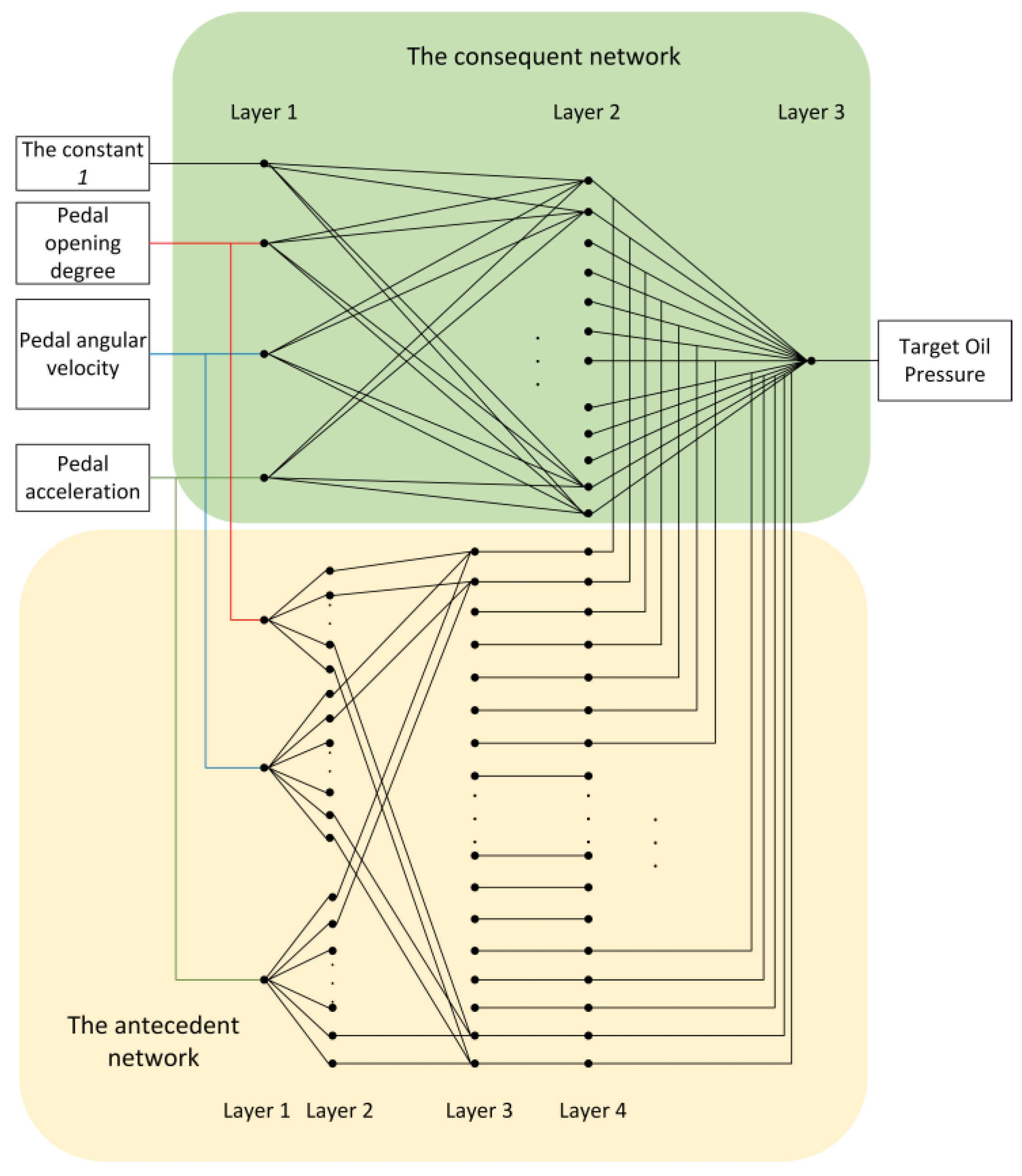
2.2.2. T-S Fuzzy Neural Network Model for Target Oil Pressure Recognition Algorithm

The Markov model, recurrent neural network model, BP neural network model, and T-S fuzzy neural network model are used for system identification and target classification [24,25,26]. The Markov model has high complexity and a long training time, which means it is not suitable for deep nonlinear feature transformation. The input of the recurrent neural network is a tree/graph structure. If there are too many parameters, then it is prone to information redundancy, resulting in gradient disappearance or explosion. The long short-term memory network has high hardware requirements and a long running time. The BP neural network involves a long training time, a large amount of computation, slow convergence speed, and the potential arising of a local minimum. The T-S fuzzy neural network has a strong adaptive ability, excellent nonlinear approximation ability and satisfactory mathematical expression characteristics, and can output an accurate linear model. The electronically assisted brake system is a mechanical, hydraulic, and electrical coupling nonlinear system, so compared with other models, the T-S fuzzy neural network model is more suitable for identifying the target oil pressure.

The T-S fuzzy system is defined by the following “if–then” rule form, where the “if” part is the antecedent of fuzzy rules and the “then” part is the consequent of fuzzy rules [27].

$$R^i: \mathrm{If} x_1 is A_1^i,x_2 \mathrm{is} A_2^i ,\dots ,x_k is A_k^i , \mathrm{then} y_i=p_0^i+p_1^i{x}_1+\dots +p_k^i{x}_k\left(j=1,2,\dots ,k\right)$$

where $R^i$ represents the rule I, $A_j^i$ is the fuzzy set of the fuzzy system, $p_j^i$ is the fuzzy system parameter, $y_i$ is the output obtained by fuzzy rules, k is the dimension of the input and i is the dimension of the output.

The T-S fuzzy neural network model for the target oil pressure recognition algorithm is divided into two parts, that is, the antecedent network and the consequent network, as shown in Figure 8. In the antecedent network, the first layer is an input layer with three neuron nodes, and the input is $\mathrm{x}=\left[x_1,x_2,x_3\right]$. They respectively represent $\mathsf{\theta }$, $\omega$ and $\mathsf{\alpha }$. The second layer is the membership function layer, where each node represents a language variable value, which is used to calculate the membership function value ${\mu }_{A_j^i}$ that states that each input component belongs to the fuzzy set of each language variable value. The fuzzy partition numbers of $x_1$, $x_2$ and $x_3$ are set to $m_1$, $m_2$ and $m_3$, so there are $q=m_1\ast m_2\ast m_3$ nodes. The Gaussian function is used as the membership function of the input variable, and the membership degree of each input variable can be calculated by Equations (1) and (2).

$${\mu }_{A_j^i}=e^{-\frac{{\left(x_j-c_j^i\right)}^2}{b_j^i}}$$

(1)

$$b_j^i=2{\sigma }_{ij}{}^2 \left(i=1,2,\dots ,q; j=1,2,3\right)$$

(2)

where $c_j^i$ and $b_j^i$ represent the center and width of the membership function, respectively, ${\sigma }_{ij}$ is the variance, j is the dimension of the input, and i is the fuzzy partition number.

The third layer of the antecedent network is the fuzzy rule layer, and each node represents a fuzzy rule, which is used to match the antecedent of the fuzzy rule and calculate the applicability of each rule. There are $q$ fuzzy rules in this layer, corresponding to $q$ nodes. The fuzzy calculation is carried out for each membership degree, and the continuous multiplication operator is used as the fuzzy operator.

$${\omega }^i={\mu }_{A_j^1}\left(x_1\right)\ast {\mu }_{A_j^2}\left(x_2\right)\ast {\mu }_{A_j^3}\left(x_3\right)$$

(3)

The fourth layer of the antecedent network is used to implement normalized computation, which has the same number of nodes as the third layer.

$$\overline{{\omega }^i}={\omega }^i/{\displaystyle \sum }_{i=1}^{\mathrm{q}}{\omega }^i$$

(4)

In the consequent network, the first layer is the input layer with four neural nodes, which are, respectively, $\mathsf{\theta }$, $\omega$ and $\mathsf{\alpha }$, and constant 1. The constant 1 is used to provide the constant term in the fuzzy rule consequent. There are $q$ nodes on the second floor, and Equation (5) is used to calculate the consequence of each rule.

$$y^i=p_0^i+p_1^i{x}_1+p_2^i{x}_2+p_3^i{x}_3$$

(5)

where $p_0^i$, $p_1^i$, $p_2^i$ and $p_3^i$ are the parameters of the consequent network.

The third layer of the consequent network is the output layer, which represents the target oil pressure and has only one node.

$$y={\displaystyle \sum }_{i=1}^{\mathrm{q}}\overline{{\omega }^i}{y}^i$$

(6)

where y is the weighted sum of the consequents of each rule, and the weighted coefficient is the normalized applicability of each fuzzy rule, that is, the output $\overline{{\omega }^i}$ of the antecedent network is used as the connection weight of the third layer.

The training of the neural network is a process of constantly correcting the weights and thresholds according to the operation error. According to the working principle of the T-S fuzzy neural network, the fuzzy system parameter $p_j^i$ is the weight value of the neural network, and the membership degree is the threshold value of the neural network, so the center $c_j^i$ of the membership function, width $b_j^i$ and weight $p_j^i$ are parameters that need to be corrected. The error cost function of the T-S fuzzy neural network can be expressed by Equation (7).

$$e=\frac{1}{2}{\left(y_d-y_c\right)}^2$$

(7)

where $y_d$ is the expected output of the neural network, $y_c$ is the actual output of the neural network, and e is the error of the two outputs.

The parameter training of the weight $p_j^i$ can be calculated with Equations (8) and (9).

$$p_j^i\left(k\right)=p_j^i\left(k-1\right)-\beta \frac{\partial e}{\partial p_j^i}$$

(8)

$$\frac{\partial e}{\partial p_j^i}=\left(y_d-y_c\right){\omega }^i/{\displaystyle \sum }_{i=1}^m{\omega }^i{x}_j$$

(9)

where $\beta$ is the learning rate.

The center $c_j^i$ and the width $b_j^i$ can be trained by Equations (10)–(13).

$$c_j^i\left(k\right)=c_j^i\left(k-1\right)-\phi \frac{\partial e}{\partial c_j^i}$$

(10)

$$b_j^i\left(k\right)=b_j^i\left(k-1\right)-\phi \frac{\partial e}{\partial b_j^i}$$

(11)

$$\frac{\partial e}{\partial c_j^i}=-{\delta }_{ij}^2\frac{2(x_j-c_j^i)}{b_j^i{}^2}$$

(12)

$$\frac{\partial e}{\partial b_j^i}=-{\delta }_{ij}^2\frac{2{(x_j-c_j^i)}^2}{b_j^i{}^3}$$

(13)

where $\phi$ is the learning rate.

2.3. Parameter Recognition of T-S Fuzzy Neural Network

2.3.1. Recognition of Antecedent Parameters by Fuzzy C-Means Clustering Algorithm

For the fuzzy C-means (FCM) clustering algorithm, membership is used to determine the degree of each data point belonging to a certain cluster, and nonlinear optimization is applied to search the local extreme points of the objective function [28]. FCM divides n dimensional vectors $x_j\left(j=1,2,\dots ,n\right)$ into $h$ fuzzy groups, and calculates the cluster center of each group to minimize the fuzzy clustering objective function. For the same set of data, the sum of membership degrees satisfies Equation (14).

$${\displaystyle \sum }_{j=1}^n{u}_{ij}=1 \left(i=1,2,\dots ,h; j=1,2,\dots ,n\right)$$

(14)

Let the sample set $X=\left[x_1,x_2,\dots ,x_n\right]$ and the fuzzy membership matrix $U={\left(u_{ij}\right)}_{h\times n}$. The clustering center matrix $V=(v_1,v_2,\dots v_h)$, n is the number of samples and h is the number of clusters. The fuzzy clustering objective function can be defined by Equations (15) and (16).

$$J\left(U,V\right)={\displaystyle \sum }_{i=1}^h{J}_i={\displaystyle \sum }_{i=1}^h{\displaystyle \sum }_{j=1}^n{u}_{ij}^m{d}_{ij}^2$$

(15)

$$d_{ij}=\Vert v_i-x_j\Vert$$

(16)

where $m\in \left[1,\infty \right]$ is a fuzzy weighted index, and $u_{ij}$ is the fuzzy membership degree of the sample $x_j$ belonging to the cluster center $v_i$, the value of which is between 0 and 1. $d_{ij}$ is the Euclidean distance between cluster center $v_i$ and sample $x_j$.

According to $\min \left(J\left(U,V\right)\right)$, the clustering center and fuzzy membership can be obtained from Equations (17) and (18).

$$v_i=\frac{{{\displaystyle \sum }}_{j=1}^n{u}_{ij}^m{x}_j}{{{\displaystyle \sum }}_{j=1}^n{u}_{ij}^m}$$

(17)

$$u_{ij}=\frac{1}{{{\displaystyle \sum }}_{k=1}^h{\left(\frac{d_{ij}}{d_{kj}}\right)}^{\raisebox{1ex}{$2$}\!\left/ \!\raisebox{-1ex}{$\left(m-1\right)$}\right.}}$$

(18)

where if $d_{ij}=0$, then $u_{ij}=1$, and $u_{kj}=0\left(k\ne i\right)$.

FCM determines the membership matrix $U$ and the clustering center $v_i$ through continuous iteration. The algorithm flow is shown in Algorithm 2.

Algorithm 2 Algorithm flow

Step 1: The number of clusters is set to h, the initial cluster center is $V^0$, the iteration stop threshold is $\epsilon$, the iterative counter q = 0, and the value of the fuzzy weighted index m is 2.

Step 2: The fuzzy membership matrix $U$ is calculated with Equation (18).

Step 3: The h cluster centers $v_i\left(i=1,2,\dots ,h\right)$ can be obtained from Equation (17).

Step 4: According to Equations (15) and (16), the value $J^q$ of the fuzzy clustering objective function is calculated. If $\Vert J^q-J^{q+1}\Vert \le \epsilon$, the algorithm is terminated, and the fuzzy membership matrix $U$ and the clustering center matrix V are obtained. Otherwise, let q = q + 1, and go to Step 2.

The element of the clustering center matrix V is the center $c_j^i$ of the T-S fuzzy neural network, and the value of $b_j^i$ can be calculated with Equations (2) and (19).

$${\sigma }_{ij}^2={\displaystyle \sum }_{k=1}^n{u}_{ik}{\left(x_j-v_i\right)}^2/{\displaystyle \sum }_{k=1}^n{u}_{ik}$$

(19)

2.3.2. Learning Rate Cosine Attenuation Strategy

The T-S fuzzy neural network uses the gradient descent method to train parameters. It is very important to choose the appropriate learning rate in the training process. The researchers use the learning rate attenuation method, that is, in the early stage of model training, a larger learning rate is used to optimize the model. The learning rate gradually decreases with the increase in the number of iterations, so as to avoid too much fluctuation in the later stage of training. The commonly used learning rate attenuation strategies include exponential attenuation, cosine attenuation, sigmoid attenuation, poly attenuation, inv attenuation, etc. [29,30,31,32].

In the exponential attenuation method, the learning rate is exponentially related to the training algebra. The exponential decay is simple and direct, and the convergence speed is fast. Its value can be calculated with Equation (20).

$${\mu }_1={\mu }_1^0\ast \left({\gamma }_1{}^t\right)$$

(20)

where ${\mu }_1$ is the current learning rate, ${\mu }_1^0$ is the initial learning rate, ${\gamma }_1$ is the attenuation coefficient, ${\gamma }_1=0.99$, and t is the current training algebra.

The cosine attenuation strategy uses the cosine function to reduce the learning rate. The learning rate first slowly decreases with the increase in the training algebra, then the decline accelerates, and finally it slowly decreases. Its value can be obtained from Equation (21).

$${\mu }_2=\frac{1}{2}{\mu }_2^0(1+cos(\frac{t\pi }{T}\left)\right)$$

(21)

where ${\mu }_2$ is the current learning rate, ${\mu }_2^0$ is the initial learning rate, T is the training algebra, and t is the current training algebra.

The sigmoid attenuation is similar to the cosine attenuation. The learning rate first decreases slowly, then decreases rapidly, and finally decreases slowly. Its value can be calculated using Equations (22) and (23).

$${\mu }_3=\frac{{\mu }_3^0}{1+e^{-{\gamma }_3\left(t-\eta \right)}}$$

(22)

$$\eta =\frac{T}{2}$$

(23)

where ${\mu }_3$ is the current learning rate, ${\mu }_3^0$ is the initial learning rate, η is the step length, ${\gamma }_3$ is the attenuation coefficient, and ${\gamma }_3=-0.01$.

In poly attenuation, the value of the learning rate first decays slowly and then decays rapidly, and this can be obtained from Equation (24).

$${\mu }_4={\mu }_4^0\ast {\left(1-\frac{t}{T}\right)}^p$$

(24)

where ${\mu }_4$ is the current learning rate, ${\mu }_4^0$ is the initial learning rate, and $p=0.25$.

In inv attenuation, the value of the learning rate drops rapidly and then slowly. Its value can be calculated with Equation (25).

$${\mu }_5={\mu }_5^0\ast {\left(1+{\gamma }_5·t\right)}^{-p}$$

(25)

where ${\mu }_5$ is the current learning rate, ${\mu }_5^0$ is the initial learning rate, ${\gamma }_5$ is the attenuation coefficient, ${\gamma }_5=0.99$, and $p=0.25$.

The initial learning rate is set to 1, T = 1000, and the attenuation effects of the five learning rates are illustrated in Figure 9.

According to Equations (8)–(13), the learning rates of T-S fuzzy neural networks are β and φ. Five learning rate attenuation strategies are used for training β and φ, respectively. The initial values of the learning rate are ${\beta }_0$ and ${\phi }_0$. The training algebra is set to 500. In total, N = 10,264 sample data points are selected, and the mean square error (MSE) is used as the loss function of the T-S fuzzy neural network.

$$\mathrm{MSE}=\frac{1}{N}{\displaystyle \sum }_{i=1}^N{\left(y_i-{\widehat{y}}_i\right)}^2 \left(i=1,2,\dots ,N\right)$$

(26)

where $y_i$ is the true value of the sample, ${\widehat{y}}_i$ is the output value of the neural network, and N is the total amount of sample data.

The curve of mean square error with the number of iterations is illustrated in Figure 10. The parameter setting and mean square error of the five learning rate attenuation strategies are shown in

Table 2. Parameters setting and results analysis of learning rate attenuation strategies.

Parameters Setting and Results	Learning Rate Attenuation Strategies
	Exp	Cosine	Sigmoid	Poly	Inv	No Attenuation
${\mathit{\beta }}_0$	0.001	0.001	0.001	0.001	0.001	0.001
${\mathit{\phi }}_0$	0.05	0.05	0.05	0.05	0.05	0.05
p	--	--	--	0.25	0.25	--
$\mathit{\gamma }$	0.99	--	-0.01	--	--	--
MSE (MPa)	0.007683	0.007027	0.013144	0.007266	0.007717	0.007761

. After 500 generations of training, the mean square error of the samples using the cosine attenuation strategy is the smallest, and its value is 0.007027 MPa. The loss function curve is smooth, without peaks and shocks. Therefore, the cosine attenuation strategy is suitable for the master cylinder target oil pressure recognition learning rate attenuation.

2.4. Training Method of Target Oil Pressure Recognition Model

The training method of the target oil pressure recognition model is illustrated in Figure 11. The T-S fuzzy neural network is trained by the sampled data of the emergency braking condition, general braking condition and no braking condition classification, respectively. Considering the braking conditions, the sampled data are divided into emergency braking data and general braking data by the braking conditions classification algorithm, and then the T-S fuzzy neural networks trained based on the data of emergency braking and general braking conditions are $T{S}_1$ and $T{S}_2$, respectively. In addition, without considering braking condition classification, the sampled data are directly used for model training to obtain the trained model $T{S}_3$.

The T-S fuzzy neural network model consists of an antecedent network and a consequent network, in which the antecedent network has four layers and the consequent network has three layers. The first layer of the antecedent network is the input layer, which takes pedal opening degree, pedal angular velocity and pedal acceleration as inputs. The second layer is used to calculate the value of the membership function, and the Gaussian function is selected as the membership function. The center $c_j^i$ and width $b_j^i$ of the Gaussian function need to be trained. The third layer is the fuzzy rule layer, which is used to match the antecedent of the fuzzy rule and calculate the applicability of each rule. The fourth layer is used to realize the normalization calculation, and the results of this layer will be used for the calculation of the second layer in the consequent network.

The first layer of the consequent network is the input layer, with the pedal opening degree, pedal angular velocity, pedal acceleration and the constant 1 as the inputs. The second layer is used to calculate the consequence of each rule, and the weight $p_j^i$ of neuron nodes is the parameter to be trained. The third layer is the output layer, of which the output is the target oil pressure.

In the T-S fuzzy neural network, the gradient descent method is used for training the parameters $c_j^i$, $b_j^i$ and $p_j^i$. In the training process, the fuzzy C-means clustering algorithm is used to calculate the initial values of $c_j^i$ and $b_j^i$, and the learning rate β and φ of the gradient descent method are processed by the learning rate cosine attenuation strategy. Finally, the trained model parameters $c_j^i$, $b_j^i$ and $p_j^i$ are obtained.

2.5. Target Oil Pressure Following Control Method

2.5.1. Traditional PID Controller and Fuzzy PID Controller

The target oil pressure results following control method based on the traditional PID or the fuzzy PID of the electronically assisted brake system are derived as shown in Figure 12. The input of the system is the target oil pressure $P_0$, which is derived from the trained T-S fuzzy neural network model, and the control amount is the actual oil pressure $P_1$. $G\left(s\right)$ is the transfer function of the motor, the transmission mechanism, the hydraulic drive unit and the brake execution unit, and $H\left(s\right)$ represents the transfer function of the feedback loop.

The oil pressure error e(k) and the error variation $e_c$(k) at time k can be calculated from the target oil pressure $P_0$ and the actual oil pressure $P_1$ by Equations (27) and (28). PID parameters $K_p$, $K_i$ and $K_d$ can be expressed by Equations (29)–(31).

$$e\left(k\right)=P_0-P_1$$

(27)

$$e_c\left(k\right)=e\left(k\right)-e\left(k-1\right)$$

(28)

$$K_p=K_{p0}+\Delta K_p$$

(29)

$$K_i=K_{i0}+\Delta K_i$$

(30)

$$K_d=K_{d0}+\Delta K_d$$

(31)

where $K_{p0}$, $K_{i0}$ and$K_{d0}$ are the initial values of the PID parameters. $\Delta K_p$, $\Delta K_i$ and $\Delta K_d$ are the changes in the PID parameters at time k.

The fuzzy subset $\left(NB,NM,NS,ZO,PS,PM,PB\right)$ is used to divide the range of $e\left(k\right)$, $e_c\left(k\right)$, $\Delta K_p$, $\Delta K_i$ and $\Delta K_d$. The fuzzy membership function uses the triangular function, and the defuzzification algorithm uses the weighted average method [33]. The fuzzy inference rules are shown in

Table 3. Fuzzy control table for $\Delta K_p$, $\Delta K_i$ and $\Delta K_d$.

Control Parameters e(k)		${\mathit{e}}_{\mathit{c}}\left(\mathit{k}\right)$
		NB	NM	NS	ZO	PS	PM	PB
$\Delta K_p$	NB	PB	PB	PM	PM	PS	PS	ZO
	NM	PB	PM	PM	PS	PS	ZO	NS
	NS	PB	PM	PM	PS	ZO	ZO	NS
	ZO	PM	PM	PS	ZO	NS	NM	NM
	PS	PS	PS	ZO	NS	NS	NM	NB
	PM	PS	ZO	NS	NM	NM	NM	NB
	PB	ZO	NM	NM	NM	NM	NB	NB
$\Delta K_i$	NB	NB	NB	NM	NM	NS	ZO	ZO
	NM	NB	NB	NM	NS	NS	ZO	ZO
	NS	NM	NM	NS	NS	ZO	PS	PS
	ZO	NM	NM	NS	ZO	PS	PS	PM
	PS	NM	NS	ZO	PS	PS	PM	PB
	PM	ZO	ZO	PS	PS	PM	PM	PB
	PB	ZO	ZO	PS	PM	PM	PB	PB
$\Delta K_d$	NB	PS	NS	NB	NB	NB	NM	PS
	NM	PS	NS	NB	NM	NM	NS	PS
	NS	ZO	NS	NM	NM	NS	NS	ZO
	ZO	ZO	NS	ZO	NS	ZO	NS	ZO
	PS	ZO	ZO	ZO	ZO	ZO	ZO	ZO
	PM	PB	NS	PS	PS	PS	PS	PB
	PB	PB	PM	PM	PM	PS	PS	PB

.

The output of incremental PID at time k can be calculated with Equations (32) and (33).

$$\Delta u\left(k\right)=K_p\left[e\left(k\right)-e\left(k-1\right)\right]+K_{i}e\left(k\right)+K_d\left[e\left(k\right)-2e\left(k-1\right)+e\left(k-2\right)\right]$$

(32)

$$u\left(k\right)=u\left(k-1\right)+\Delta u$$

(33)

where $\Delta u$ is the motor target torque increment at time k, u(k) is the motor target torque at time k, and u(k − 1) is the motor target torque at the previous moment.

2.5.2. Correction Method of Target Oil Pressure

In the process of vehicle braking, in order to prevent dangerous situations such as wheel locking and side–slip, it is necessary to make the vehicle obtain the maximum braking force, shorten the braking distance, and improve the braking direction stability and handling stability [34]. The target oil pressure following control method is improved by combining the slip ratio control method to improve the accuracy of the oil pressure control and improve the braking performance of the controller.

According to the tire ground model, road adhesion is related to the slip ratio, which can be expressed by the relationship between the lateral adhesion coefficient, the longitudinal adhesion coefficient and the slip ratio [35], as shown in Figure 13. The slip ratio is the ratio of the speed difference between the vehicle speed and the wheel speed to the vehicle speed, which can be used to measure the degree of wheel slip and is expressed by Equation (34) [36].

$${\lambda }_c=\frac{v_c-{\omega }_c\ast r_c}{v_c}$$

(34)

where ${\lambda }_c$ is the tire slip ratio, $v_c$ is the vehicle speed, ${\omega }_c$ is the wheel rotation angular velocity, and $r_c$ is the wheel rolling radius.

As shown in Figure 13, the region from the beginning of braking to the slip ratio ${\lambda }_c={\lambda }_0$ is a stable area, at which the lateral adhesion coefficient gradually decreases and the longitudinal adhesion coefficient gradually increases. When the slip ratio ${\lambda }_c$ increases to ${\lambda }_0$, the longitudinal adhesion coefficient reaches the maximum value, and the lateral adhesion coefficient also remains at a high value. At this time, the longitudinal force of the tire reaches the maximum value, which can obtain a large ground braking force and ensure the braking safety of the vehicle. The region from ${\lambda }_0$ to ${\lambda }_c=1$ is unstable. In this region, with the increase in the slip ratio, the longitudinal adhesion coefficient and lateral adhesion coefficient decrease greatly, and the vehicle gradually loses stability. When the slip ratio ${\lambda }_c$ increases to ${\lambda }_c=1$, the longitudinal adhesion coefficient reaches ${\mu }_s$, the lateral adhesion coefficient is close to 0, the wheel is completely locked, and the vehicle slips sideways, which makes it prone to accidents.

Therefore, in the process of vehicle braking, when the slip ratio ${\lambda }_c$ is maintained at ${\lambda }_0$, the longitudinal adhesion coefficient is the largest, and the lateral adhesion coefficient is also high. The vehicle can obtain the best braking efficiency and has good lateral stability. ${\lambda }_0$ is the optimal slip ratio, which is theoretically equal to 0.2. However, due to the differences in road surfaces and braking conditions, ${\lambda }_0$ fluctuates in the range of $\left[{\lambda }_{min},{\lambda }_{max}\right]$ [37]. In short, the braking performance of the system can be improved by using an appropriate control strategy to keep the slip ratio in the range of $\left[{\lambda }_{min},{\lambda }_{max}\right]$.

We combine the slip ratio control algorithm with the target oil pressure following control method, as shown in Figure 14. The improved target oil pressure following control method is composed of the slip ratio control loop and the oil pressure control loop.

In the slip ratio control loop, the inputs are vehicle speed $v_c$, wheel angular velocity ${\omega }_c$ and oil pressure P, and the output is target oil pressure $P_0$. The oil pressure P comes from the trained T-S fuzzy neural network model. $G_2\left(s\right)$ is the transfer function of the wheel, and $H_2\left(s\right)$ represents the transfer function of the feedback loop of vehicle speed and wheel angular velocity. As shown in Figure 14b, the actual slip ratio ${\lambda }_c$ is calculated by the vehicle speed $v_c$, wheel angular velocity ${\omega }_c$ and wheel rolling radius $r_c$, as shown in Equation (35).

$$P_0=\{\begin{array}{c}P+k_r\ast t {\lambda }_c<{\lambda }_{min}\\ P {\lambda }_{min}\le {\lambda }_c\le {\lambda }_{max}\\ P-k_f\ast t {\lambda }_c>{\lambda }_{max}\end{array}$$

(35)

where $k_r$ is the brake oil pressure growth rate, $k_f$ is the brake oil pressure reduction rate, and t is the sampling time.

In the oil pressure control loop, the input is the target oil pressure $P_0$, which is the output of the slip ratio control algorithm, and the output is the actual oil pressure $P_1$.$G_1\left(s\right)$ is the transfer function of the motor, the transmission mechanism, the hydraulic drive unit and the brake execution unit, and $H_1\left(s\right)$ represents the transfer function of the feedback loop of the oil pressure. The fuzzy PID controller and incremental PID algorithm of the oil pressure control loop are the same as those in Section 2.5.1.

3. Model Training and Experiments

3.1. Training of Target Oil Pressure Recognition Model

In total, 22,398 groups of brake data are collected from the test bench shown in Figure 4, which are divided into 11,140 groups of data under emergency braking conditions and 11,258 groups of data under general braking conditions. Firstly, the 7438 groups of the data derived under emergency braking conditions are selected as the training set, and 3702 groups are used as the testing set to train the model $T{S}_1$; the results are illustrated in Figure 15. Secondly, the 7698 groups of data derived under general braking conditions are selected as the training set, and 3560 groups are used as the testing set to train the model $T{S}_2$; the results are illustrated in Figure 16. Finally, the 22,398 groups of data derived under the two braking conditions are merged, and then divided into 15,136 groups of training set data and 7262 groups of testing set data, which are used to train the model $T{S}_3$, and the results are illustrated in Figure 17.

Comparing the above training results, as shown in

Table 4. Oil pressure recognition results for the training set and testing set.

Error Evaluation Indexes		Braking Conditions Classification
		Emergency Braking Condition $\left(\mathit{T}{\mathit{S}}_1\right)$	General Braking Condition $\left(\mathit{T}{\mathit{S}}_2\right)$	Without Braking Conditions Classification $\left(\mathit{T}{\mathit{S}}_3\right)$
Training set	Sample size	7374	7698	15136
	Maximum error (MPa)	0.4403	0.6295	1.2273
	Minimum error (MPa)	$5.9139\times {10}^{-7}$	$7.9529\times {10}^{-7}$	$1.2136\times {10}^{-6}$
	MSE (MPa)	0.0049	0.0038	0.0216
Testing set	Sample size	3702	3560	7262
	Maximum error (MPa)	0.6841	0.7705	1.2684
	Minimum error (MPa)	$1.6700\times {10}^{-5}$	$7.6543\times {10}^{-5}$	$8.1190\times {10}^{-6}$
	MSE (MPa)	0.0351	0.0396	0.1062

, in the training results of models $T{S}_1$ and $T{S}_2$, the mean square error and the error range are significantly smaller than in the results for model $T{S}_3$, so the use of braking conditions classification can improve the accuracy of the brake master cylinder target oil pressure recognition model.

3.2. Experiments of Target Oil Pressure Following Control

The test bench is mainly made up of a brake pedal, mechanical transmission module, power motor module, angle sensor, oil pressure sensor and data acquisition card. The mechanical transmission module is composed of a coupling, worm gear and rack. The power motor module is composed of a power motor, controller and driver. The power-assisted motor is a LESSEL ACM8075V48H-A4 low-voltage servo motor (Leadshine, Shenzhen, China). The driver is a LESSEL LD2-RS7020 series (Leadshine, Shenzhen, China). The angle sensor is a WT901CM attitude sensor (Witmotion, Shenzhen, China). The oil pressure sensor is a 0~30MPa pressure sensor (LONTROL, Hangzhou, China). The data acquisition card is an NI PS-15 series acquisition card (National Instruments, Austin, TX, USA). The host computer software system communicates with the motor driver through the Modbus RTU communication protocol. The target oil pressure following control test bench is illustrated in Figure 18 and Figure 19.

The target oil pressure results derived following control methods based on a traditional PID controller and fuzzy PID controller are used in experiments, respectively. The sampling frequency is 50Hz. According to the simulation experiment, the control parameters of the traditional PID controller are $K_p=0.055$, $K_i=0.0055$ and $K_d=0.025$. The initial parameters of the fuzzy PID controller are $K_{p0}=0.055$, $K_{i0}=0.0055$ and $K_{d0}=0.025$. The value ranges of e(k) and $e_c\left(\mathrm{k}\right)$ are set to [−6,6] and [−6,6]. The ranges of $\Delta K_p$, $\Delta K_i$ and $\Delta K_d$ are set to [−0.015,0.015], [−0.0015,0.0015] and [−0.005,0.005]. The experimental results are divided into emergency braking conditions and general braking conditions, which are illustrated in Figure 20, Figure 21, Figure 22 and Figure 23.

The following error of the oil pressure in the oil pressure following control method can be seen in

Table 5. The experimental results of oil pressure following control.

PID Controller	Error Evaluation Indexes	Braking Conditions Classification
		Emergency Braking Condition			General Braking Condition
		Oil Pressure Rising	Oil Pressure Holding	Oil Pressure Falling	Oil Pressure Rising	Oil Pressure Holding	Oil Pressure Falling
Traditional PID Controller	Maximum error (MPa)	1.8480	0.2191	0.6542	0.4424	0.1157	1.7369
	Minimum error (MPa)	$4.61\times {10}^{-4}$	$2.03\times {10}^{-5}$	$5.92\times {10}^{-5}$	$2.54\times {10}^{-5}$	$3.15\times {10}^{-5}$	$8.60\times {10}^{-4}$
	MSE (MPa)	0.3325	0.0406	0.0778	0.0448	0.0354	0.0654
Fuzzy PID Controller	Maximum error (MPa)	0.4789	0.2609	0.3335	0.3022	0.0328	0.5443
	Minimum error (MPa)	$2.08\times {10}^{-5}$	$1.99\times {10}^{-6}$	$3.0\times {10}^{-5}$	$3.77\times {10}^{-6}$	$5.51\times {10}^{-6}$	$4.33\times {10}^{-6}$
	MSE (MPa)	0.1411	0.0411	0.0610	0.0266	0.0224	0.0266

. In the case of the traditional PID controller, the oil pressure following error is in the range of ($2.03\times {10}^{-5}$,1.8480) under emergency braking conditions and general braking conditions. The stage of oil pressure holding has high control precision, but the oil pressure errors in the stages of oil pressure rising and falling are quite large, and the maximum value is 1.8480MPa. This shows that the traditional PID controller struggles to maintain high control accuracy in the oil pressure rising and falling stages, and it struggles to cope with the rapid change in the oil pressure value. In the case of the fuzzy PID controller, the oil pressure following error is in the range of ($1.99\times {10}^{-6}$,0.5443). Under the general braking conditions, in the stages of oil pressure rising, holding and falling, all have high control precision. Under the emergency braking conditions, the error range of the rapid rise stage of oil pressure is slightly larger, but is still within the allowable range of engineering errors. To sum up, the fuzzy PID controller has higher control accuracy than the traditional PID controller in the following control of the target oil pressure, and is more able to cope with rapid changes in the oil pressure value.

4. Conclusions

The research proposes a method to realize oil pressure identification and the control of oil pressure in the master cylinder without relying on an accurate system model. The experiment verifies the effectiveness of the method under emergency braking and general braking conditions. Using the target oil pressure of the electronically assisted brake system obtained by referring to the braking characteristics of other mature braking systems is an effective and fast method to obtain control objectives; moreover, the target oil pressure taken as the input of the master cylinder oil pressure following control method with fuzzy PID is also a feasible technical route. The main conclusions of this article are as follows:

• Pedal opening degree, pedal angular velocity and pedal acceleration can be used as the basis for the classification of braking conditions;
• The sample data of emergency braking conditions and general braking conditions obviously differ in terms of pedal opening change rate and pedal acceleration, and therefore, the two braking conditions need to be distinguished, and the neural network parameters trained respectively under emergency braking and general braking conditions can significantly improve the accuracy of identification;
• The initial values of the T-S fuzzy neural network model parameters $c_j^i$, $b_j^i$, $p_j^i$ trained by the fuzzy C-means clustering algorithm are helpful in improving the training accuracy of the model compared with the random initialization of each parameter. Using the learning rate cosine decay strategy is beneficial to speeding up the training rate in the early stage of model training, jumping out of the local minimum, improving the accuracy of the model in the later stage of training, and helping the model converge;
• The fuzzy PID control and incremental PID control algorithm can realize the torque control of the power motor without relying on an accurate model of the electronically assisted brake system, and can also realize the following control of the oil pressure. This method has better control accuracy than the traditional PID controller.

There are some shortcomings of this study:

• When using the fuzzy C-means clustering algorithm to calculate the initial values of $c_j^i$ and $b_j^i$, the number of cluster centers is artificially selected, which involves subjective factors, and whether the number of cluster centers is set reasonably will affect the clustering results;
• Due to the limitations of the experimental conditions, the vehicle status information is not involved in the brake data collection and brake control algorithm verification experiments, and the correction method of target oil pressure cannot be verified because of the lack of related test data.

The above shortcomings will be points to improve in future research.

References

1. Wang, X.; Wu, X.; Cheng, S.; Shi, J.; Ping, X.; Yue, W. Design and experiment of control architecture and adaptive dual-loop controller for brake-by-wire system with an electric booster. IEEE Trans. Transp. Electrif. 2020, 6, 1236–1252. [Google Scholar] [CrossRef]
2. Yu, Z.; Han, W.; Xu, S.; Xiong, L. Development status of hydraulic pressure control of electronic hydraulic brake system. J. Mech. Eng. 2017, 53, 1–15. [Google Scholar] [CrossRef]
3. Chen, Q.; Shao, H.; Liu, Y.; Xiao, Y.; Wang, N.; Shu, Q. Hydraulic-pressure-following control of an electronic hydraulic brake system based on a fuzzy proportional and integral controller. Eng. Appl. Comput. Fluid Mech. 2020, 14, 1228–1236. [Google Scholar] [CrossRef]
4. Büchler, R. Future brake systems and Technologies–Mk C1®–Continental’s brake system for future vehicle concepts. In Proceedings of the 7th International Munich Chassis Symposium 2016, 1st ed., 16 August 2016; Springer Vieweg: Wiesbaden, Germany. Available online: https://link.springer.com/chapter/10.1007/978-3-658-14219-3_45 (accessed on 1 November 2022).
5. Hua, Y.; Jiang, H.; Tian, H.; Xu, X.; Chen, L. A comparative study of clustering analysis method for driver’s steering intention classification and identification under different typical conditions. Appl. Sci. 2017, 7, 1014. [Google Scholar] [CrossRef]
6. Wang, S.; Zhao, X.; Yu, Q.; Yuan, T. Identification of driver braking intention based on long short-term memory (LSTM) network. IEEE Access 2020, 8, 180422–180432. [Google Scholar] [CrossRef]
7. Fang, E.; Zhang, D.; Cheng, Z. Research on recognition method and application of passenger car driver’s braking intention. Shanghai Auto 2016, 1, 49–53. [Google Scholar]
8. Ju, J.; Bi, L.; Feleke, A.G. Noninvasive neural signal-based detection of soft and emergency braking intentions of drivers. Biomed. Signal Process. Control 2022, 72, 9. [Google Scholar] [CrossRef]
9. Zheng, H.; Ma, S.; Fang, L.; Zhao, W.; Zhu, T. Braking intention recognition algorithm based on electronic braking system in commercial vehicles. Int. J. Heavy Veh. Syst. 2019, 26, 268–290. [Google Scholar] [CrossRef]
10. Gu, Y.; Xie, J.; Liu, H.; Yang, Y.; Tan, Y.; Chen, L. Evaluation and analysis of comprehensive performance of a brake pedal based on an improved analytic hierarchy process. Proc. Inst. Mech. Eng. Part D J. Automob. Eng. 2021, 235, 2636–2648. [Google Scholar] [CrossRef]
11. Meng, D.; Zhang, L.; Yu, Z. A dynamic model for brake pedal feel analysis in passenger cars. Proc. Inst. Mech. Eng. Part D J. Automob. Eng. 2016, 230, 955–968. [Google Scholar] [CrossRef]
12. Pei, X.; Pan, H.; Chen, Z.; Guo, X.; Yang, B. Coordinated control strategy of electro-hydraulic braking for energy regeneration. Control. Eng. Pract. 2020, 96, 104324. [Google Scholar] [CrossRef]
13. Tavernini, D.; Vacca, F.; Metzler, M.; Savitski, D.; Ivanov, V.; Gruber, P.; Hartavi, A.E.; Dhaens, M.; Sorniotti, A. An explicit nonlinear model predictive abs controller for electro-hydraulic braking systems. IEEE Trans. Ind. Electron. 2020, 67, 3990–4001. [Google Scholar] [CrossRef]
14. Nadeau, J.; Micheau, P.; Boisvert, M. Collaborative control of a dual electro-hydraulic regenerative brake system for a rear-wheel-drive electric vehicle. Proc. Inst. Mech. Eng. Part D J. Automob. Eng. 2019, 233, 1035–1046. [Google Scholar] [CrossRef]
15. Wu, J.; Zhang, H.; He, R.; Chen, R.; Chen, H. A Mechatronic Brake Booster for Electric Vehicles: Design, Control, and Experiment. IEEE Trans. Veh. Technol. 2020, 69, 7040–7053. [Google Scholar] [CrossRef]
16. Chu, L.; Xu, Y.; Zhao, D.; Chang, C. Research on pressure control algorithm of regenerative braking system for highly automated driving vehicles. World Electr. Veh. J. 2021, 12, 112. [Google Scholar] [CrossRef]
17. Chen, P.; Wu, J.; Zhao, J.; He, R. Design and power assisted braking control of a novel electromechanical brake booster. SAE Int. J. Passeng. Cars-Electron. Electr. Syst. 2018, 11, 171–181. [Google Scholar] [CrossRef]
18. Meng, B.; Yang, F.; Liu, J.; Wang, Y. A survey of brake-by-wire system for intelligent connected electric vehicles. IEEE Access 2020, 8, 225424–225436. [Google Scholar] [CrossRef]
19. Zhu, F.; Guo, H.; Xu, W.; Liu, J.; Chen, H.; Lv, Y. Modeling of a novel Brake-by-Wire (BBW) system for electric vehicle based on dual Closed—loop PID. In Proceedings of the 31st Chinese Control And Decision Conference (CCDC), Nanchang, China, 3–5 June 2019. [Google Scholar]
20. Zhao, X.; Li, L.; Wang, X.; Mei, M.; Liu, C.; Song, J. Braking force decoupling control without pressure sensor for a novel series regenerative brake system. Proc. Inst. Mech. Eng. Part D J. Automob. Eng. 2019, 233, 1750–1766. [Google Scholar] [CrossRef]
21. Yang, I.; Choi, K.; Huh, K. Development of an electric booster system using sliding mode control for improved braking performance. Int. J. Automot. 2012, 13, 1005–1011. [Google Scholar] [CrossRef]
22. Aksjonov, A.; Vodovozov, V.; Raud, Z. Improving energy recovery in blended antilock braking systems of electric vehicles. In Proceedings of the 16th IEEE International Conference on Industrial Informatics (INDIN), Univ Porto, Fac Engn, Porto, Portugal, 18–20 July 2018. [Google Scholar]
23. Zhao, J.; Deng, Z.; Zhu, B.; Chang, T.; Chen, Z. Hydraulic pressure control of electric power braking system based on RBF network sliding mode. J. Mech. Eng. 2020, 56, 106–114. [Google Scholar]
24. Chae, H.; Kang, C.; Kim, B.; Kim, J.; Chung, C.; Choi, J. Autonomous braking system via deep reinforcement learning. In Proceedings of the 2017 IEEE 20th International conference on intelligent transportation systems (ITSC), Yokohama, Japan, 16–19 October 2017. [Google Scholar]
25. Min, K.; Yeon, K.; Jo, Y.; Sim, G.; Sunwoo, M.; Han, M. Vehicle deceleration prediction based on deep neural network at braking conditions. Int. J. Automot. 2020, 21, 91–102. [Google Scholar] [CrossRef]
26. Xia, G.; Li, J.; Tang, X.; Zhao, L.; Sun, B. Layered control of forklift lateral stability based on Takagi-Sugeno fuzzy neural network. Proc. Inst. Mech. Eng. Part D J. Automob. Eng. 2021, 235, 1767–1780. [Google Scholar] [CrossRef]
27. Li, J. Research on robot motion control based on variable structure fuzzy neural network based on T-S model. In Proceedings of the 5th International Conference on Environmental Science and Material Application (ESMA), Xi’an, China, 15–16 December 2019. [Google Scholar]
28. Wang, N.; Yao, W.; Zhao, Y.; Chen, X. Bayesian calibration of computer models based on Takagi-Sugeno fuzzy models. Comput. Methods Appl. Mech. Eng. 2021, 378, 113724. [Google Scholar] [CrossRef]
29. Lu, M.; Peng, T.; Yue, G.; Ma, B.; Liao, X. Dual-channel hybrid neural network for modulation recognition. IEEE Access 2021, 9, 76260–76269. [Google Scholar] [CrossRef]
30. Bhattacharyya, A.; Chatterjee, S.; Sen, S.; Sinitca, A.; Kaplun, D.; Sarkar, R. A deep learning model for classifying human facial expressions from infrared thermal images. Sci. Rep. 2021, 11, 1–17. [Google Scholar]
31. Nakamura, K.; Derbel, B.; Won, K.; Hong, B. Learning-rate annealing methods for deep neural networks. Electronics 2021, 10, 2029. [Google Scholar] [CrossRef]
32. Wang, W.; Lee, C.; Liu, J.; Colakoglu, T.; Peng, W. An empirical study of cyclical learning rate on neural machine translation. Nat. Lang. Eng. 2022, 1–21. [Google Scholar] [CrossRef]
33. Vodovozov, V.; Petlenkov, E.; Aksjonov, A.; Raud, Z. Simulation study of electric vehicles at fuzzy PID control of braking torque. In Proceedings of the Informatics in Control, Automation and Robotics: 17th International Conference, ICINCO 2020 Lieusaint, Paris, France, 7–9 July 2020. [Google Scholar]
34. Umnitsyn, A.; Bakhmutov, S.V. Intelligent anti-lock braking system of electric vehicle with the possibility of mixed braking using fuzzy logic. J. Phys. Conf. Ser. 2021, 2061, 2021. [Google Scholar] [CrossRef]
35. He, Y.; Lu, C.; Shen, J.; Yuan, C. A second-order slip model for constraint backstepping control of antilock braking system based on Burckhardt’s model. Int. J. Model. Simul. 2020, 40, 130–142. [Google Scholar] [CrossRef]
36. Cao, K.; Hu, M.; Wang, D.; Qiao, S.; Guo, C.; Fu, C.; Zhou, A. All-Wheel-Drive Torque Distribution Strategy for Electric Vehicle Optimal Efficiency Considering Tire Slip. IEEE Access 2021, 9, 25245–25257. [Google Scholar] [CrossRef]
37. Gowda, D.V.; Ramachandra, A.C. Slip ratio control of anti-lock braking system with bang-bang controller. Int. J. Comput. Tech. 2017, 4, 97–104. [Google Scholar]
Figure 1. The electronically assisted brake system structure.
Machines 11 00183 g001
Figure 2. The framework of research content.
Machines 11 00183 g002
Figure 3. Composition of braking data acquisition test bench: 1. WT901CM attitude sensor, 2. brake pedal, 3. PC Software, 4. NI acquisition card, 5. NI acquisition card chassis, 6. oil pressure sensor, 7. DC power supply, 8. oil pipe, 9. brake caliper.
Machines 11 00183 g003
Figure 4. Brake data acquisition test bench: 1. NI acquisition card chassis, 2. NI acquisition card, 3. DC power supply, 4. WT901CM attitude sensor, 5. brake pedal, 6. test bench bracket, 7. Bosch’s electric-assisted braking system, 8. brake caliper, 9. DC power supply, 10. oil pressure sensor.
Machines 11 00183 g004
Figure 5. Sampled data under general braking conditions: (a) Sampled data of actual oil pressure and θ . (b) Sampled data of ω and α .
Machines 11 00183 g005
Figure 6. Sampled data under emergency braking conditions: (a) Sampled data of actual oil pressure and θ . (b) Sampled data of ω and α .
Machines 11 00183 g006
Figure 7. Braking conditions classification algorithm.
Machines 11 00183 g007
Figure 8. T-S fuzzy neural network model for target oil pressure recognition algorithm.
Machines 11 00183 g008
Figure 9. Results of five learning rate attenuation strategies.
Machines 11 00183 g009
Figure 10. Mean square error of learning rate attenuation strategies in oil pressure recognition.
Machines 11 00183 g010
Figure 11. The training process of the target oil pressure recognition model.
Machines 11 00183 g011
Figure 12. Block diagram of the target oil pressure following control: (a) Traditional PID controller. (b) Fuzzy PID controller.
Machines 11 00183 g012
Figure 13. The relationship between the brake road adhesion coefficient and the slip ratio.
Machines 11 00183 g013
Figure 14. Improved target oil pressure following control method: (a) The combination of target oil pressure following control method and slip ratio control algorithm. (b) Slip ratio control algorithm.
Machines 11 00183 g014
Figure 15. Oil pressure recognition results of the training set and testing set under emergency braking conditions: (a) Actual oil pressure, target oil pressure and oil pressure identification error of training set. (b) Oil pressure identification error of training set. (c) Actual oil pressure, target oil pressure and oil pressure identification error of testing set. (d) Oil pressure identification error of testing set.
Machines 11 00183 g015
Figure 16. Oil pressure recognition results of the training set and testing set under general braking conditions: (a) Actual oil pressure, target oil pressure and oil pressure identification error of training set. (b) Oil pressure identification error of training set. (c) Actual oil pressure, target oil pressure and oil pressure identification error of testing set. (d) Oil pressure identification error of testing set.
Machines 11 00183 g016
Figure 17. Oil pressure recognition results of the training set and testing set without braking conditions classification: (a) Actual oil pressure, target oil pressure and oil pressure identification error of training set. (b) Oil pressure identification error of training set. (c) Actual oil pressure, target oil pressure and oil pressure identification error of testing set. (d) Oil pressure identification error of testing set.
Machines 11 00183 g017
Figure 18. Composition of target oil pressure following control test bench: 1. WT901CM attitude sensor, 2. brake pedal, 3. worm wheel, 4. worm, 5. coupling, 6. servo motor, 7. DC power supply, 8. motor driver, 9. oil cup, 10. spline shaft, 11. rack, 12. master cylinder push rod, 13. master cylinder, 14. PC Software, 15. NI acquisition card, 16. NI acquisition card chassis, 17. oil pressure sensor, 18. oil pipe, 19. DC power supply, 20. brake caliper.
Machines 11 00183 g018
Figure 19. Target oil pressure following control test bench: 1. NI acquisition card chassis, 2. NI acquisition card, 3. DC power supply, 4. WT901CM attitude sensor, 5. brake pedal, 6. test bench bracket, 7. Electric-assisted braking system shell, 8. oil cup, 9. master cylinder, 10. coupling, 11. servo motor, 12. brake caliper, 13. DC power supply, 14. motor driver, 15. oil pressure sensor.
Machines 11 00183 g019
Figure 20. Results of oil pressure following control based on traditional PID controller under emergency braking conditions: (a) Target oil pressure, actual oil pressure and oil pressure error. (b) Oil pressure error.
Machines 11 00183 g020
Figure 21. Results of oil pressure following control based on traditional PID controller under general braking conditions: (a) Target oil pressure, actual oil pressure and oil pressure error. (b) Oil pressure error.
Machines 11 00183 g021
Figure 22. Results of oil pressure following control based on fuzzy PID controller under emergency braking conditions: (a) Target oil pressure, actual oil pressure and oil pressure error. (b) Oil pressure error.
Machines 11 00183 g022
Figure 23. Results of oil pressure following control based on fuzzy PID controller under general braking conditions: (a) Target oil pressure, actual oil pressure and oil pressure error. (b) Oil pressure error.
Machines 11 00183 g023