Abstract
The design parameters are the most momentous factors in carrying out performance matching. For complex electromechanical products with a large number of design parameters, determining a set of critical design parameters which have a great influence on the performance is the premise of performance matching. In this paper, from a systematic perspective, a screening method of critical design parameters based on energy and a causal model is proposed. Since energy is the driving force of the product operation to achieve performance, the design parameters affect the performance through energy flow in the product. Therefore, the causal model among design parameters, characteristic energy, and performance is established, where its path coefficients are determined based on the quantitative calculation of the energy flow simulation model. Then, the performance pertinence is defined and calculated to describe the comprehensive influence of the design parameters on performance and to screen the critical parameters. Finally, the performance matching process is presented to support the performance matching. With a refrigerator as an example, 5 parameters were screened from 11 variable design parameters, and day power consumption decreased by 6.85%, which verifies the effectiveness of the method.
1. Introduction
Performance, as the essential factor that determines the value and market competitiveness of the product, has always been the focus of the design field [1,2]. For the mechanical product, its performance depends on design parameters, operating conditions, maintenance levels, and other factors. Thereinto, the design parameters determine the attributes of the product and the ability to adapt to the environment, so they are the most momentous factors in carrying out performance matching [3].
On account of these facts, Papalambros [4] described the performance design as a problem of achieving target performance through design parameter optimization under certain performance constraints and attempted to establish a relationship between the design parameters and the performance. Some scholars, such as Deng [5] and Ma [6], took specific products, such as missile weapon equipment and wind turbines, as objects and realized performance design through combination optimization of related design parameters. However, there are a large number of design parameters affecting the performance of complex mechanical and electrical products, and the relationships between the design parameters and the performance are extremely complicated so that in the design process, the performance objectives and constraints are generally difficult to be expressed directly with the design parameters in the form of functions, and the combination optimization of design parameters is extremely time-consuming. Therefore, it is really essential to identify the critical parameters for electromechanical products among a large number of design parameters.
At present, numerous methods and pieces of research are devoted to solving the issue of screening critical design parameters. The pertinence matrix method mainly realizes the screening of critical parameters by constructing the relationship matrix of different structural levels among performance parameters, function modules, and component design parameters. For instance, Shin et al. [7] and Ma et al. [8] identified the design parameters to be improved by establishing the correlation matrix between design parameters and performance. Moreover, sensitivity analysis [9] is another method to quantitatively describe the importance of design parameters on the variation of performance parameters by establishing functional relationships, where the design parameters with high sensitivity coefficients are obtained for improvement. There are, however, usually great difficulties in establishing functional relationships between design parameters and performance parameters. Hence the researchers [10,11,12] established an approximate mapping relationship with the nonlinear mapping ability of the artificial neural networks to derive the calculation equation of sensitivity. In addition, the relationships between design parameters and performance parameters in the method based on internal mechanism analysis [13] are mainly established through physical models, such as dynamic equations, structural wear models, etc. Then, the critical design parameters are obtained through the degradation trend of performance parameters. For example, Liu [14] proposed a wave structure for shaping the leading edge of the blade based on the bionic concept to improve turbomachine performance and reduce turbomachine noise. Walter [15] studied the effect of the aerodynamic preload and the minimum clearance on the dynamic performance and the stability characteristic of the bump-type foil air bearing.
As for the studies above, the pertinence matrix is relatively dependent on the engineering experience of the designers, which leads to different quantitative standards from different experts for the correlation analysis, while the training process of sensitivity analysis with neural networks requires a large number of samples, which is of low interpretability and causes high test costs in the field of mechanical product design. Compared with the neural network sensitivity analysis and the pertinence matrix method, the internal mechanism analysis is more explanatory; however, the mechanism analysis tends to focus on a certain internal function module rather than the entire product, leading to the failure of the whole system matching after the weak link is strengthened. Therefore, it is indispensable for screening critical design parameters of electromechanical products to establish an explicable, systematic, and mechanism-based model based on quantitative studies between the design parameters and the performance from a systematic perspective.
In order to build a more appropriate screening model, the analysis of the relationships between design parameters and performance is the precondition. In general, describing that the performance response is related to the choice of the design parameters is a correlation problem, while describing that the design parameters affect the performance response and analyzing how much this effect is, involves causality. Correlation is any relationship that can be defined in terms of the joint distribution of observed variables, but causation cannot be defined in terms of the data distribution alone, and the processes that produce the data need to be clarified. Obviously, for complex electromechanical products, their performance responses are the results of the combination of the design parameters, which means that there exist causal relationships between design parameters and performance. Therefore, the causality is more accurate to analyze the effect of design parameters on performance through a causal model, and intensive study on their causality will be conducive to the screening of the critical design parameters. The causal model [16], widely used in life science [17], economics [18], sociology [19], and artificial intelligence [20,21,22], is an analytical method that analyzes the causal relationship between variables with path analysis technology. Furthermore, it is used to verify the assumed causal relationships between variables through observable data. In the mechanical field, Gu [23] has applied a causal chain to the fault diagnosis model of steam turbines based on fault mechanism. However, when the causal model is applied to screening critical design parameters, if the causal model is established only by assigning the path coefficients between the design parameters and the performance parameters, it will be difficult to avoid the dependency on the engineering experience. To solve the problem, it is best to combine the causal relationships between the design parameters and the performance with the operational mechanism of the product.
Energy is the driving force behind the operation of energy-consuming electromechanical products to achieve functions and performance [24]. Growing research [25] on control co-design has reflected the importance of the change of energy flow among the product on the performance. Many scholars have studied the modeling methods of the energy in the conceptual design stage [26,27,28] and detailed design stage [29]. Thereinto, TRIZ [30] proposed the basic principle of “matter-field” and revealed that the product function was realized through the material (such as the parts and the modules) and the field interaction (such as the mechanical force, the electricity, and the magnetic force) between the materials. The literature [31] constructed an energy flow expression mode based on the energy flow element (EFE) in which functions (F), design variables (v), characteristic energy (Ec), energy variable quantity (), and interface parameters (q) were defined in order to describe the energy function characteristics of parts in functional realization, as shown in Figure 1a. With the directed line segment as the energy transmission between EFEs, the energy flow model of products can be established by EFEs. For example, Figure 1b illustrates that in the refrigerator, the energy was transmitted as the refrigerant flowed from compressor EFE to condenser EFE through a pipeline so that the interface parameters at the compressor output were the same as those at the condenser input. With the energy expression mode for the refrigerator, the design parameters (theoretical volumetric capacity Vth, volume efficiency , and isentropic efficiency of compressor, tube length Lc and inner diameter Dc of condenser) influence the energy flow via the interface parameters (mass flow rate mr, pressure pr, temperature Tr, and flow velocity vr of the refrigerant), and consequently, affect its refrigerating capacity, so that the quantitative simulation between design parameters, characteristic energy and performance can also be established to support the systematic performance matching. To sum up, there are causal relationships among design parameters, energy and performance parameters, with the design parameters and performance bonding together by the operation mechanism via the energy.
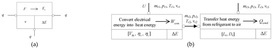
Figure 1.
Energy flow expression mode [31]: (a) Energy flow element; (b) Energy transmission between compressor and condenser.
Therefore, in order to take the statistical approach and the product’s internal mechanism into consideration jointly, the screening method of critical design parameters based on energy and a causal model is presented in this paper. Based on the energy flow model of electromechanical products in the literature [31], the characteristic energy is introduced to establish the causal model among design parameters, characteristic energy, and performance parameters on the basis of the quantitative relationships between design parameters and characteristic energy, and between characteristic parameters and performance parameters through simulation. A group of critical design parameters is screened to support the performance matching through the performance pertinence, which is defined to evaluate the influence of the design parameters on the performance parameters. Finally, the refrigerator design is taken as an example to verify the effectiveness of the method to screen the critical parameters of mechanical and electrical product performance design based on energy and the causal model.
2. Methods
In this section, the causal model is firstly summarized, and then the modeling method of screening critical design parameters based on energy and the causal model is presented. Product performance includes economic performance, technical performance, and social performance. Since the causal model in this paper is based on energy as a bridge, the performance concerned in this research is technical performance related to energy, and the research object is mainly energy-consuming mechanical and electrical products.
2.1. The Causal Model
The causal model is expressed by the path graph, which has the capability of expressing and analyzing the relationships between multiple variables, especially the indirect influence between variables. A path graph with five variables is shown in Figure 2.
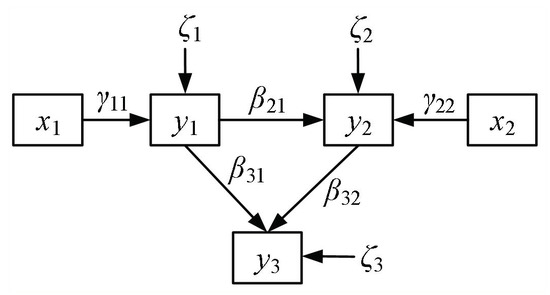
Figure 2.
The path graph in a general form.
In the path graph, the boxes represent the variables, and the arrows represent the causal relationships between variables. For instance, if x1 has an effect on y1, an arrow is drawn from x1 to y1. The numbers on the arrows, called path coefficients, represent the degree of influence between variables. It is common for the result variable to come first and the cause variable to come second in path coefficient subscripts. According to the relationships in the path graph, variables defined as acting but not affected are called exogenous variables (x1, x2), while variables affected by other variables are called endogenous variables (y1, y2, y3). It can be seen that there may also be a correlation between endogenous variables. Generally, the path coefficient from the exogenous variable to the endogenous variable is expressed by γ, while the path coefficient between endogenous variables is expressed by β.
In general, the causal model can be described in the form of the following structural equation:
where X represents a vector composed of exogenous variables, Y represents a vector composed of endogenous variables, B is a matrix composed of path coefficients from endogenous variables to endogenous variables, Γ is a matrix composed of path coefficients from exogenous variables to endogenous variables, and ζ is the error vector of the endogenous variables.
As shown in Figure 2, the causal model composed of two exogenous variables and three endogenous variables are as follows: , . Furthermore, assuming that each error of the endogenous variables is independent, that is, the covariance between them is 0, then the covariance matrix of the error Ψ is a diagonal matrix: . The causal model, similar to Figure 2, of which B is the lower triangular matrix and Ψ is the diagonal matrix, is called the recursive model. Recursive models have the following two advantages:
- All of the recursive models are recognizable, and the path coefficient solutions can be determined by building structural equations;
- The unbiased estimation of each coefficient in the structural equation can be obtained with the least square method in the recursive model. Each structural equation is estimated based on the least square method, and the estimated regression coefficient is the path coefficient between variables.
The establishment and analysis methods of the causal model generally include the following steps:
- 3.
- Model setting and parameters estimation
Firstly, the variables involved in the model are determined and divided into exogenous variables and endogenous variables. Then, the path graph between the exogenous variables and the endogenous variables is established and written as a structural model. After that, the path coefficients of each path, that is, the coefficients on each arrow, are estimated based on the sample parameters. For the recursive model, the least square method can be used for each equation to estimate all the path coefficients.
- 4.
- Model inspection and evaluation
The model inspection and evaluation are used to test whether the preset causal relationship is tenable based on the results of parameter estimation. Similar to regression analysis, what needs to be tested is whether the parameter has significance to zero. Generally, the t-test standard in regression analysis can be used to calculate the critical ratio and significance probability of the path coefficient, and then the significance level can be tested through the t-distribution.
- 5.
- Effect decomposition
In the path analysis, the effect refers to the influence of the cause variable on the result variable. Its mathematical expression is the covariance between variables, which can be expressed by the standardized path coefficient between variables. The effect can be divided into direct effect and indirect effect. The direct effect reflects the influence of the cause variable directly on the result variable, while the indirect effect reflects the influence of the cause variable indirectly on the result variable through several intermediate variables, which is equal to the sum of the product of the path coefficients from the cause variable through all intermediate variables to the result variable. The total effect is the sum of direct and indirect effects:
Total Effect = Direct Effect + Indirect Effect
For example, in Figure 2, the direct effect of variable y1 on y3 is β31, and the indirect effect produced by y2 is β21β32, so the total effect of y1 on y3 can be expressed as the sum of direct and indirect effects, namely β31 + β21β32.
2.2. Establishing Screening Method of Critical Design Parameters Based on Energy Analysis and Causal Model
In combination with the modality of the causal model, the process of establishing the screening method for critical design parameters based on energy and the causal model is shown in Figure 3. Firstly, on the basis of the expression of energy flow, the design parameters, characteristic energy, and performance are determined. Secondly, the interaction among design parameters, characteristic energy, and performance is established via a path graph according to the causal model analysis method. Thirdly, the path coefficients of the above factors are determined by using the path analysis technique and experimental design. Then, the performance pertinence index is defined to describe the comprehensive influence degree of the design parameters on the performance and is calculated by analyzing the total effect of design parameters on the performance through different paths with the effect decomposition method. Finally, a group of critical design parameters with matching relationships under the current focus on performance is obtained by comparing the performance pertinence.
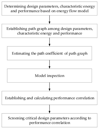
Figure 3.
The process of establishing screening method for critical design parameters.
2.2.1. Establishing Path Graph
In the energy flow expression, the design parameters are the cause of the characteristic energy and performance, so they are exogenous variables. The characteristic energy is generated by the design parameters, and the performance is the result of the action of the characteristic energy, both of which are endogenous variables. Therefore, a path graph describing the relationships between design parameters, characteristic energy, and performance can be established, as shown in Figure 4.
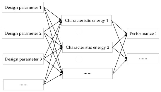
Figure 4.
The path graph based on the energy flow expression.
Based on the general causal model modeling theory, the characteristics of the energy flow model realized for the performance of energy-consuming electromechanical products have the following assumptions:
- 6.
- Recursive form
It is assumed that the relationships among design parameters, characteristic energy, and performance are unidirectional, and there is no loop or feedback relationship, which satisfies the assumption of the recursive model. The assumption of the recursive model is based on the fact that in the performance realization, the energy flow model constructs the bridge between design parameters and performance, and the characteristic energy is the interpretation of the performance realization degree from the perspective of energy, so it is a progressive relationship layer by layer.
- 7.
- No pertinence among design parameters
For electromechanical products, the design parameters are determined by the designer. In combination with the Independence Axiom of Axiomatic Design, although there may be geometric constraints and other pertinences among design parameters, it still can be considered that each design parameter can be valued without constraints within a certain range. The assumption is of great significance for analyzing the characteristic energy and performance response when design parameters change and can contribute to establishing the structural equation which accurately reflects the influence of design parameters on characteristic energy and performance.
- 8.
- Path assumption
In the causal model shown in Figure 4, the arrowhead line segment represents the action path between variables, and there is a hypothetical causal relationship between the two variables. It can be seen from the definition that the causal model method is not to explore the existing pertinence between variables but to verify the presumed correlation between variables through observable data. Therefore, it is usually possible to establish a full-relationship model among design parameters, characteristic energy, and performance, and then the validity of the path relationship is verified through the path verification technique. However, a large number of variables will make this method require a number of verification calculations. In this case, some paths can be assumed to exist or not exist according to the product’s prior knowledge, thus simplifying the model.
2.2.2. Parameter Estimation
Parameter estimation refers to the analysis of the degree of influence between variables in Figure 4, and the influence is expressed by the path coefficients. The larger the standardized path coefficient is, the greater the relative influence of the cause variable on the result variable is. Since the path graph of the energy flow model satisfies the recursive model hypothesis, so it is recognizable, and the least square method can be used to obtain the unbiased estimation of each path coefficient, respectively. After multiple regression for each equation in the structural equations, the (partial) regression coefficient is the corresponding path coefficient.
Suppose that some result variable is y, and the reason variables that have a structural relationship with y include x1, x2, …, xn, then the structural relation among them is shown in Equation (3):
where β1, β2, …, βn are the path coefficients, and β0 is the constant term. To obtain the values of the path coefficients and the constant terms, p sets of observations are required. It can be seen that the relationships among design parameters, characteristic energy, and performance in the energy flow model based on the causal model are established through the actual state of the product. This method is completely the simulation and interpretation of the system characteristics rather than the establishing of the functional relationships among the three variables. The final concern is the degree of influence among different factors, so the method is conducive to achieving a good balance between the amount of calculation and the accuracy of the results.
In order to establish the sample containing p-group observed values, different methods are supposed to be adopted for different design stages of complex electromechanical products. In the stage of new product development and verification, the characteristic energy and performance response of the design parameters under different values can be solved by the algebraic method with a numerical simulation model or finite element method. In the product improvement stage, by combining different parts and their design parameters, the characteristic energy and performance response can be obtained through the prototype test.
When establishing samples, the value method of design parameters can be carried out through the experimental design, where the variables are generally called factors, and the possible values of the variables are called levels. When there are few factors, all combinations of levels between factors can be tested by means of a comprehensive test. As the number of factors increases, conducting a full test requires considerable manpower and time. At this time, the most commonly used experimental design methods include orthogonal design [32] and uniform design [33]. Both orthogonal test tables and uniform test tables can be consulted in common test design textbooks.
After that, the p group observed values of the structural equation shown in Equation (3) are obtained by simulation or experiment: . Equation (3) can be written in matrix form:
Suppose , , , then the unbiased estimation of the path coefficient β1, β2, …, βn is obtained with the least square method:
where is the unbiased estimation of the path coefficient from variable x to y.
The path coefficients obtained by the least square method above are non-standardized and reflect the dimensional relationships between the cause variables and the result variables; that is, the change of the cause unit variable will lead to the change of the corresponding unit result variable. However, the nonstandard path coefficients are not easy to compare the relative importance of one variable to another because of the dimensional differences between different variables. Therefore, the path coefficients obtained by Equation (5) need to be standardized with the following formula:
where βj is the estimated coefficient of the variable xj; is the estimated standard error of the coefficient βj; Sy is the estimated standard deviation of the variable y. The least squares estimation and the normalization process of the coefficients can be implemented using the software AMOS.
2.2.3. Model Inspection
The model inspection is to verify whether the regression equation in the causal model really describes the pertinence law between variables. According to the results of the significance analysis, some non-significant paths in the original path hypothesis are removed to make the model more reflective of the characteristics of the system. The significance test is conducted by a t-test.
Construct the t statistic:
where is the estimate of βj, cjj can be obtained by the matrix , i, j = 0, 1, 2, …, p, and is the regression standard deviation which can be obtained by the following formula:
The bilateral inspection threshold is tα/2. When |tj| ≥ tα/2, βj is not zero significantly, so the cause variable has a significant effect on the result variable; conversely, when |tj| < tα/2, βj is considered to be zero, and the effect of the cause variable on the result variable is not significant.
In order to facilitate the judgment, the significance probability, usually called the p-value, is introduced. The relationship between the t-value and p-value is as follows:
that is, the p-value is equal to the probability that the t-value is greater than its test value. The p-value can be estimated by AMOS software when the p-value is ≤ α, |t| ≥ tα/2, and the regression effect is significant. When the p-value is > α, |t| < tα/2, and the regression effect is not significant. Therefore, checking the t distribution table can be omitted if t is replaced with P. Moreover, the relative significance of different variables can be compared with the p-value, which is convenient for testing and modifying the model. For example, the significance test result of the path coefficient γ11 on the left of Figure 5 is as follows: p-value > 0.05 when the path coefficient is not significant, indicating that the action path and path coefficient from x1 to y1 cannot really reflect the causal relationship between them, but only the quantitative relationship due to the statistical relationship. Therefore, it is necessary to remove the insignificant path and modify the model to obtain the model shown on the right. It is worth noting that after removing the non-significant path, the parameter estimation and significance test of the path model need to be re-performed. Under normal circumstances, the path with the largest p-value is removed successively after the significance test of the initial model until all the paths meet the significance condition.
P(|t| > |t-test value|) = p-value
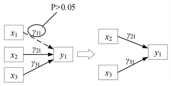
Figure 5.
Significance test and correction of the path coefficient.
2.2.4. Performance Pertinence Calculation
Based on the path analysis of the above causal model, the action path and the influence degree of design parameters on characteristic energy and performance are obtained. In order to quantitatively evaluate the degree of influence of the design parameters on performance, and construct the performance-matching optimization problem, the concept of performance pertinence is defined as follows:
Definition 1:
The performance pertinence of the design parameters refers to the degree of influence on the performance, which is defined as the relative change of performance when there is a certain relative change in design parameters.
According to the definition of performance pertinence, the higher the performance pertinence of the design parameters is, the greater the impact of their changes on performance is. The matching relationships between the design parameters with high-performance importance are critical in building and solving the performance-matching problem. In order to evaluate the importance of the design parameters reflected in the performance by the characteristic energy, the performance pertinence of the design parameters is calculated with the effect decomposition method.
Suppose that the design parameters contained in the energy flow model are (v1, v2, …, vn), the characteristic energy is (Ec1, Ec2, …, Ecm), the performance is (P1, P2, …, Pl), the normalized path coefficient of the design parameter vi to the characteristic energy Ecj is γji, and the normalized path coefficient of the characteristic energy Eci to the performance Pj is βji. In particular, if a path does not exist, its corresponding path coefficient is 0. According to the definition of the performance pertinence, the performance pertinence of the design parameter vi on the performance Pj is the total effect of vi on Pj, equal to the sum of the product of the path coefficients that vi indirectly acts on Pj through all Eci, as shown in the following Equation:
For example, in the path graph shown in Figure 6, its path coefficients are the standardized path coefficients that pass the significance test. The performance pertinence of the design parameters v1, v2, and v3 on performance P1 is calculated as follows:
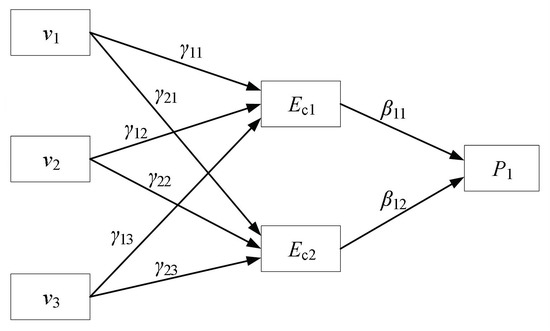
Figure 6.
Performance pertinence calculation with effect decomposition.
It is important to note that since the path coefficient can be positive and negative (positive path coefficient represents positive pertinence, and negative path coefficient represents negative pertinence), the performance pertinence calculated by Equation (10) can also be positive and negative. Therefore, the design parameter with the larger absolute value of performance pertinence has a stronger influence on the performance and should be taken as the focus of the matching design.
After calculating the performance pertinence of the design parameters on the specified performance, the relationship or conflict between different performance objectives should be considered comprehensively. The performance pertinence of the design parameters on different performances is weighted according to the weight, then the comprehensive performance pertinence of design parameters on all concerned performances can be obtained. In order to avoid the counteract of the positive and negative performance pertinence, it is necessary to take the absolute value of the performance pertinence. For example, with the weight vector introduced, the comprehensive performance pertinence of the design parameter vi on all performance objectives is expressed as follows:
2.3. Performance Matching Process for Energy-Consuming Electromechanical Products
By calculating the comprehensive performance pertinence, the design parameters that have great influences on the performance can be screened as a whole. Using this group of design parameters to construct the performance matching problem can effectively realize comprehensive matching optimization. Therefore, the performance matching process of energy-consuming electromechanical products based on energy and causal model is shown in Figure 7:
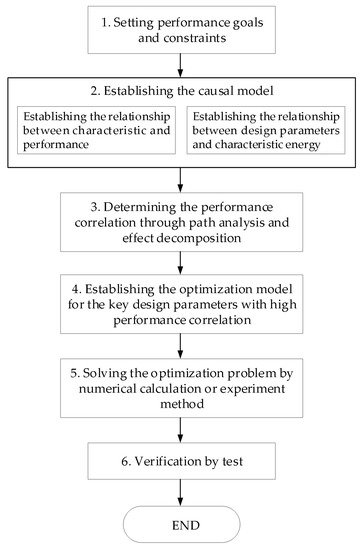
Figure 7.
The performance matching process based on energy and causal model.
3. Case Study and Discussion
The energy consumption and refrigeration performance of household refrigerators are the basis of their competitiveness, which are also the focus of major refrigerator manufacturers. In this section, an energy efficiency improving development example of a refrigerator, of which the volume is 278 L, day power consumption is 0.68 kW·h/24 h, the operating rate is 70%, the suction temperature is 20 °C, and temperature uniformity is 2.5 °C−1, is selected to verify the effectiveness of the critical design parameters screening method proposed in this paper based on energy and a causal model.
3.1. Establishing the Energy Flow Model of the Refrigerator
The design parameters and the characteristic energy of the refrigerator are shown in the energy flow model in Figure 8 [31]. In the energy efficiency improving development process of the refrigerator, the characteristics of power saving and consumption reduction (day power consumption ECday, energy efficiency ratio COP) is defined as the performance objective, and the food preservation characteristics (temperature uniformity °C−1) and the running state characteristics (operating rate R and suction temperature Tsuc) are defined as the performance constraints [31].
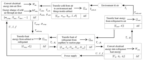
Figure 8.
Energy flow model of refrigerator [31].
The energy flow model of the refrigerator includes six EFEs (compressor, condenser, evaporator, capillary-suction tube, compartment, and air duct system). Based on the energy flow model, the simulation model of each EFE is established. Taking the compressor EFE as an example, the simulation model is as follows:
The specific enthalpy of the outlet:
The flow rate of the refrigerant:
The power consumption of the compressor:
The heat dissipated:
where is the specific capacity at the inlet (m3/kg), is the specific enthalpy of isentropic compression from the suction state to the exhaust pressure, and are the heat transfer coefficient and the heat transfer area of air heat dissipation by the compressor, respectively.
The simulation models of other EFEs are established referring to that of the compressor, according to which the Newton iteration method is used to establish the iteration model. As shown in Figure 9, the operating state parameters of the system under different design parameter combinations can be obtained.
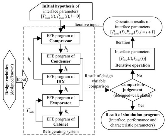
Figure 9.
Iterative process of refrigerator simulation based on energy flow model [31].
In order to verify the above simulation model, an existing refrigerator is used to carry out experiments. When the refrigerator reaches a stable running state, the simulated and measured results are compared, as shown in Table 1.

Table 1.
Experimental comparison results.
The temperature deviation is less than 2 °C, and the compressor power consumption deviation is less than 2W, which is within the acceptable range. Therefore, the refrigerator simulation model based on the energy flow model can support the following design parameters screening.
Aiming at the concerned performance of the refrigerator, based on the energy flow model, the path graph among design parameters, characteristic energy, and performance are established, the performance pertinence of design parameters is calculated through path analysis and effect decomposition, and then the critical design parameters are screened out. By carrying out the optimization design of these design parameters, the performance matching of the refrigerator is realized.
3.2. Establishing the Causal Model of Refrigerator
In the actual development process of the refrigerator, some of the above EFE design parameters exist as standard parameters, such as the number of condenser rows and the fin type of evaporator, etc. The other part of the design parameters is determined by the designer during the design process to achieve performance optimization. Performance matching is the determination of an optimal set of these variable design parameters so that the performance meets the design objectives and constraints. The compartment EFE is defined by the box volume stipulated by the design task and the foam layer thickness stipulated by the standard, so the design parameters of compartment EFE are considered to be known before the design, not as a matching object. According to experience, it is assumed that there is a path relationship or no path relationship between variables. In case of no path relationship, suppose that there was a path relationship that was corrected. Thus, the path graph among refrigerator variables is established, as shown in Figure 10, including design parameters, characteristic energy, and performance of variables involved in performance matching.
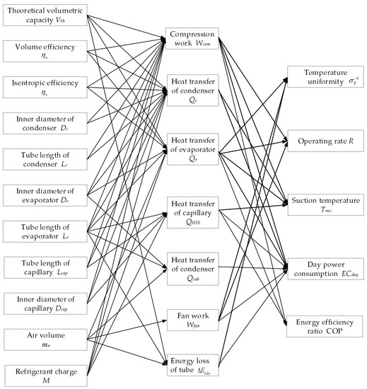
Figure 10.
The path graph of refrigerator performance realization.
As shown in Table 2, eleven design parameters are set with three levels each, and the orthogonal design is carried out according to L27(313). For each set of combinations, interface state parameters are obtained by simulation method, and then characteristic energy and performance responses are calculated by the energy characteristic equation. The sample containing design parameter combinations, characteristic energy, and performance responses can be used to estimate the causal model shown in Figure 9.
Table 2.
The orthogonal experimental group of design parameters.
Based on the sample data, the path coefficients in the causal model are estimated by Equations (4)–(6). The paths with insignificant path effects are removed one by one with the significance test method shown in Equations (7)–(9), and then the path graph model is modified. The revised path graph and standardized path coefficient are shown in Table 3.
Table 3.
The estimation results of path coefficient.
3.3. Performance Pertinence Calculation and Critical Design Parameters Screening
According to Equation (10), the performance pertinence of design parameters on each performance is calculated. Then, AHP [34] is adopted to determine the weight of each performance index (:ECday:COP:R:Tsuc) = (0.2:0.3:0.2:0.15:0.15). Finally, the comprehensive performance pertinence of each design parameter is calculated with Equation (14), as shown in Table 4.
Table 4.
The calculation results of the comprehensive performance pertinence.
According to Table 4, taking the theoretical volumetric capacity Vth of the compressor as an example, it plays a decisive role in the day power consumption ECday and operating rate R, which is approximately equal to the influence trend (Figure 10) of Vth on ECday and R when carrying out parameters analysis. Compared with the influence trend in Figure 11, the method gives a comprehensive index among various performance indexes, and the causality is more straightforward than the correlation relationship. So, the results of the performance pertinence are relatively reliable. In addition, the air circulation volume ma, meanwhile, plays a critical role in the uniformity of the box. The above two design parameters should be selected as the critical parameters for performance matching. In addition to the performance pertinence, the cost of changing design parameters also needs to be considered when selecting other critical design parameters. For example, the tube length Le of the evaporator can be adjusted in the cutting process, while the adjustment of the inner diameter De involves the change of the mold, which will bring a high cost. In addition, changing the inner diameter of the evaporator will affect the adjacent part and its port parameters, such as the capillary, which may lead to a series of adjustments of the manufacturing links of the adjacent parts. Therefore, when the performance pertinence of tube length is close to that of inner diameter, the tube length is preferred as its critical design parameter. Furthermore, though the comprehensive performance pertinences of Dc and Dcap are bigger than that of Lcap, Lcap will be the preferred critical parameter.
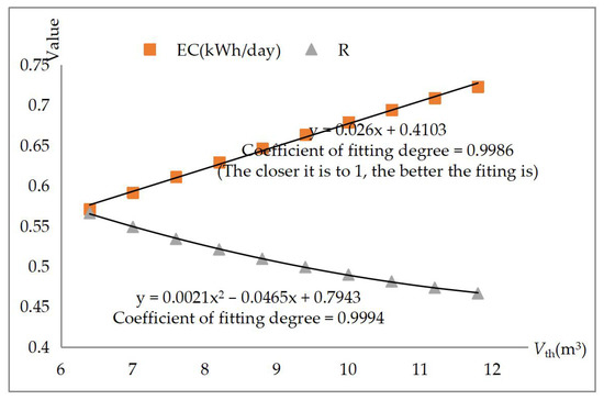
Figure 11.
The influence trend of Vth on ECday and R.
Finally, the screened critical design parameters with significant influence on the performance include compressor theoretical volumetric capacity Vth, refrigerant charge M, length of evaporator tube Le, length of capillary tube Lcap, and air volume of fan ma.
3.4. Matching Design and Verification
The critical design parameters (compressor theoretical volumetric capacity Vth, refrigerant charge M, length of evaporator tube Le, length of capillary tube Lcap, and air volume of fan ma) with higher performance pertinence are easier to be changed and screened to carry out the matching design to reach the development goal. According to the value range of each design parameter, the value of these critical design parameters is set as shown in Table 5.
Table 5.
The value of the critical design parameters.
The uniform design method is adopted to obtain the performance response under each group of design parameter combinations based on the simulation model.
With the factors Vth, M, Lcap, Le, and ma replaced by the letters A, B, C, D, and E, respectively, the regression model between the design parameters and the performance response is established with the daily power consumption ECday as the performance objective and the other performance parameters as the performance constraints. The first-order linear regression is adopted as follows:
The above equation set illustrates the relationship between performance and critical design parameters, which contribute to the performance matching via the critical design parameters. For example, the daily power consumption ECday is positively correlated with compressor theoretical volumetric capacity Vth, length of evaporator tube Le, length of capillary tube Lcap, and air volume of fan ma; thereinto, the air volume of the fan has the greatest influence and needs more attention during the designing process. Both and of the above approximate models are greater than 90%, indicating a good degree of model fitting. According to the fitting model, the following problems are optimized:
Using mixed integer linear programming, the results satisfying the optimization conditions are calculated as follows: Vth = 9.52 cm3, M = 40.7 g, Le = 5.8 m, Lcap = 2.3 m, ma = 0.022 kg/s. The corresponding performance response is calculated as follows: ECday = 0.6088 kW∙h/24 h, R = 69.42%, Tsuc = 16.56 °C, = 2.54 °C−1.
According to the optimized design parameters, the original refrigerator (278 L) is improved and tested based on the requirements of the type tests. Figure 12a shows the type of test room, which covers the basic experimental requirements, such as ambient temperature control device, humidity control device, etc. Power and temperature signals are collected, as shown in Figure 12b, and three temperature points are set to measure the temperature uniformity in Figure 12c. The type test room is controlled via the system of Figure 12d, and after 8000 min, the refrigerator enters the stable operation state. The test results of the new refrigerator prototype are recorded and shown in Figure 13, where the day power consumption and the operating rate can be calculated according to the power curve, and the temperature uniformity can be obtained from the curves of temperature points 1–3.
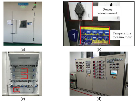
Figure 12.
Test equipment: (a) Type test room; (b) Signal collection device of power and temperature; (c) Temperature point for temperature uniformity; (d) Control processing system.
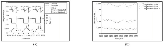
Figure 13.
The test results of the new refrigerator prototype: (a) Periodic operating parameters; (b) Testing of temperature uniformity.
The product indexes obtained from the test results are shown in Table 6, where the calculated value refers to the results from the simulation model, the test value refers to the experimental results of the improved refrigerator prototype, and the reference value refers to the performance indexes of the original refrigerator.
Table 6.
The test results of the refrigerator prototype.
As shown in Table 6, the test value is approximately equal to the calculated value except that there is some difference in the suction temperature, which may be caused by the difficult-to-calculate heat leakage and eddy current caused by the tiny structure of the outlet. In spite of this, all indexes of the prototype still meet the requirements of the optimization problems, among which the day power consumption has decreased by 6.85%. Therefore, the number of design parameters to be considered in performance matching is reduced from 11 to 5 with the help of the screening method of refrigerator critical design parameters based on the causal model. On the basis of realizing effective performance matching, direct calculation and combination of a large number of component parameters are avoided so that the manpower, financial resources, and time consumed in design are reduced, which proves the effectiveness of the proposed method.
4. Conclusions
Based on the energy flow expression of electromechanical products, a causal model to screen the critical design parameters is presented and is verified through the design process of a refrigerator in this paper. The statistical method and mechanism analysis are combined systematically based on quantitative studies among design parameters, energy, and performance in this method. The specific conclusions are as follows:
- Based on the energy analysis, the causal model is established with the causal relationships among the design parameters, characteristic energy, and performance analyzed, and the path coefficients in the path graph are determined by parameters estimation and model inspection, which is supported by the quantitative calculation based on mechanism analysis.
- Based on the causal model, with the path and the degree of influence of design parameters on characteristic energy and performance analyzed, an index performance pertinence is defined to quantitatively evaluate the influence degree of the design parameters on performance. A calculation method of the performance pertinence is established through effect decomposition to support the selection of critical design parameters. Finally, a performance-matching process of electromechanical products based on the causal model is presented.
- Taking the refrigerator as an example, eleven variable design parameters, such as the compressor theoretical volumetric capacity Vth, are selected to carry out the critical design parameters screening based on the causal model, with the daily power consumption ECday as the performance objective, the temperature uniformity, the operating rate R, and the suction temperature Tsuc as the performance constraints. The five critical design parameters with significant influence on the performance, including compressor theoretical volumetric capacity Vth, refrigerant charge M, length of evaporator tube Le, length of capillary tube Lcap, and air volume of fan ma, are screened to support the performance matching of the refrigerator. All indexes of the prototype meet the design requirements, among which the daily power consumption has decreased by 6.85%. That is, the number of design parameters to be considered in performance matching is reduced from 11 to 5 with the help of the screening method of refrigerator critical design parameters based on the causal model. Therefore, the method in this paper is effective.
The method proposed in this paper takes energy as the bridge to establish a causal model among design parameters, characteristic energy, and performance, defines the total causal effect of design parameters on performance as the performance pertinence, and takes it as the basis for parameter screening. Based on the energy flow model, this method is more systematic than the variable selection method based on performance degradation. In addition, compared with the variable screening model completely based on statistics, this method transforms the completely symmetric correlation between variables into the asymmetric causal relationship from design variables to performance, which has more clear physical significance and provides a new idea for variable screening of energy-consuming mechanical and electrical products.
However, this method can only be used to design and improve the energy-related technical performance of energy-consuming mechanical and electrical products. Meanwhile, the analysis of causality can be further studied.
Author Contributions
Conceptualization, X.W. and D.X.; methodology, X.W.; software, X.W.; validation, X.W.; writing—original draft preparation, X.W.; writing—review and editing, X.W. and D.X.; supervision, D.X.; project administration, D.X. All authors have read and agreed to the published version of the manuscript.
Funding
This research received no external funding.
Institutional Review Board Statement
Not applicable.
Informed Consent Statement
Not applicable.
Data Availability Statement
Not applicable.
Conflicts of Interest
The authors declare no conflict of interest.
References
- Xing, D.Q. Study on Method of Performance Driving Design for Complex Mechanical Product and Typical Application. Ph.D. Thesis, Tianjin University, Tianjin, China, 2010. [Google Scholar]
- Zheng, H.; Feng, Y.X.; Gao, Y.C.; Tan, J.R. The solving process of conceptual design for complex product based on performance evolution. J. Mech. Eng. 2018, 54, 214–223. [Google Scholar] [CrossRef]
- Chu, X.N.; Chen, H.S.; Ma, Z.H. Identification of critical design parameter for mechanical products based on performance data. J. Mech. Eng. 2021, 57, 185–196. [Google Scholar]
- Papalambros, P.Y.; Wilde, D.J. Principles of Optimal Design: Modeling and Computation, 3rd ed.; Cambridge University Press: Cambridge, UK, 2017; pp. 1–45. [Google Scholar]
- Deng, G.Q.; Kuang, S.Q.; Lv, Y.J.; Hao, G.Y.; Qi, S.J.; An, Y.W. The Integration Design Parameters Selection Method of Equipment Performance and Testing. In Man-Machine-Environment System Engineering, Proceedings of the 19th International Conference on Man-Machine-Environment System Engineering (MMESE), Shanghai, China, 19–21 October 2019; Long, S., Dhillon, B.S., Eds.; Springer: Singapore, 2020; pp. 307–314. [Google Scholar]
- Ma, B.B. Identification of Critical Parameters Based on Wind Turbines Performance Degradation. Master’s Thesis, Shanghai Jiaotong University, Shanghai, China, 2020. [Google Scholar]
- Shin, J.H.; Kiritsis, D.; Xirouchakis, P. Design modification supporting method based on product usage data in closed-loop PLM. Int. J. Comput. Integr. Manuf. 2015, 28, 551–568. [Google Scholar] [CrossRef]
- Ma, H.Z.; Chu, X.N.; Xue, D.Y. An integrated approach for design improvement based on analysis of time-dependent product usage data. J. Mech. Des. 2017, 139, 111401. [Google Scholar] [CrossRef]
- Borgonovo, E.; Plischke, E. Sensitivity analysis: A review of recent advances. Eur. J. Oper. Res. 2016, 248, 869–887. [Google Scholar] [CrossRef]
- Shuai, K.; Li, Z.; Zhou, L.; Wang, J. Multi-objective optimization design of PMASynRM based on RBF neural network. J. Phys. Conf. Ser. 2022, 2183, 012013. [Google Scholar] [CrossRef]
- Pan, L.X.; Novak, L.; Lehky, D.; Novak, D.; Cao, M.S. Neural network ensemble-based sensitivity analysis in structural engineering: Comparison of selected methods and the influence of statistical pertinence. Comput. Struct. 2021, 242, 106376. [Google Scholar] [CrossRef]
- Zhang, C.; Guo, Y.; Li, M. Review of Development and Application of Artificial Neural Network Models. Comput. Eng. Appl. 2021, 57, 57–69. [Google Scholar]
- Fomin, A.S.; Paramonov, M.E. Structural and Kinematic Analysis of a Mechanism for Internal Surfaces Processing. J. Mach. Manuf. Reliab. 2019, 48, 292–298. [Google Scholar] [CrossRef]
- Liu, H.; Lu, Y.; Yang, J.; Wang, X.; Ju, J.; Tu, J.; Yang, Z.; Wang, H.; Lai, X. Aeroacoustic Optimization of the Bionic Leading Edge of a Typical Blade for Performance Improvement. Machines 2021, 9, 175. [Google Scholar] [CrossRef]
- Walter, F.; Sinapius, M. Influence of Aerodynamic Preloads and Clearance on the Dynamic Performance and Stability Characteristic of the Bump-Type Foil Air Bearing. Machines 2021, 9, 178. [Google Scholar] [CrossRef]
- Glymour, C.; Zhang, K.; Spirtes, P. Review of causal discovery methods based on graphical models. Front. Genet. 2019, 10, 524. [Google Scholar] [CrossRef]
- Laubach, Z.M.; Murray, E.J.; Hoke, K.L.; Safran, R.J.; Perng, E. A biologist’s guide to model selection and causal inference. Proc. R. Soc. B Biol. Sci. 2021, 288, 20202815. [Google Scholar] [CrossRef] [PubMed]
- Huo, K.; Kelly, K.; Webb, A. The beneficial learning effects of combining a hypothesis- testing mindset with a causal model. Account. Rev. 2022, 97, 325–348. [Google Scholar] [CrossRef]
- Banerjee, T.; Paul, A.; Srikanth, V.; Strumke, I. Causal connections between socioeconomic disparities and covid-19 in the USA. Sci. Rep. 2022, 12, 15827. [Google Scholar] [CrossRef] [PubMed]
- Sahoh, B.; Haruehansapong, K.; Kliangkhlao, M. Causal artificial intelligence for high-stakes decisions: The design and development of a causal machine learning model. IEEE Access 2022, 10, 24327–24339. [Google Scholar] [CrossRef]
- Yann, L.C. How Does the Brain Learn so Much so Quickly? Cognitive Computational Neuroscience (CCN). 2017. Available online: https://www.youtube.com/watch?v=cWzi38-vDbE&t=150s (accessed on 14 December 2022).
- Pearl, J. Theoretical Impediments to Machine Learning with Seven Sparks from the Causal Revolution. In Proceedings of the Eleventh ACM International Conference on Web Search and Data Mining, Marina Del Rey, CA, USA, 5–9 February 2018. [Google Scholar]
- Gu, Y.J.; Yang, N.; Chen, D.C.; Song, L. Study on intelligent fault diagnosis of steam turbines using fault causality information. Noise Vib. Control 2019, 39, 12–19. [Google Scholar]
- Xiang, D.; Mou, P.; Shen, Y.H.; Wang, X. Green Design Method of Energy Consuming Electromechanical Products Based on Energy Flow, 1st ed.; China Machine Press: Beijing, China, 2022; pp. 20–25. [Google Scholar]
- Peters, D.L.; Papalambros, P.Y.; Ulsoy, A.G. Relationship between coupling and the controllability Grammian in co-design problems. Mechatronics 2015, 29, 36–45. [Google Scholar] [CrossRef]
- Pahl, G.; Beitz, W. Engineering Design; Design Council: London, UK, 1984. [Google Scholar]
- Stone, R.B. Towards a Theory of Modular Design. Ph.D. Thesis, University of Texas at Austin, Austin, TX, USA, 1998. [Google Scholar]
- Feghali, J.E.; Sandou, G.; Guéguen, H.; Haessig, P.; Faille, D. Energy-Based Method to Simplify Complex Multi-Energy Modelica Models. In Proceedings of the 14th Modelica Conference 2021, Linköping, Sweden, 20–24 September 2021. [Google Scholar]
- Wang, H.L.; Xiang, D.; Jiang, L.F.; Duan, G.H.; Zhang, H.C. Improvement of vehicle crashworthiness for full frontal impact based on energy flow analysis. Adv. Mater. Res. 2010, 139, 1365–1369. [Google Scholar] [CrossRef]
- Altshuller, G. 40 Principles: TRIZ Criticals to Technical Innovation, 1st ed.; Technical Innovation Center, Inc.: Worcester, MA, USA, 1998. [Google Scholar]
- Wang, X.; Xiang, D. Energy Flow Modelling Method of Energy Efficiency Improvement for Power-Using Electromechanical Products. Energies 2022, 15, 5240. [Google Scholar] [CrossRef]
- Ghaderpour, E. Constructions for Orthogonal Designs Using Signed Group Orthogonal Designs. Discret. Math. 2017, 341, 277–285. [Google Scholar] [CrossRef]
- Fang, K.T.; Li, R.; Sudjianto, A. Uniform Experimental Design. In Design and Modeling for Computer Experiments, 1st ed.; Chapman & Hall/CRC Press: Boca Raton, FL, USA, 2006; pp. 67–104. [Google Scholar]
- Guo, J.Y.; Zhang, Z.B.; Sun, Q.Y. Study and applications of analytic hierarchy process. China Saf. Sci. J. 2008, 18, 148–153. [Google Scholar]


Disclaimer/Publisher’s Note: The statements, opinions and data contained in all publications are solely those of the individual author(s) and contributor(s) and not of MDPI and/or the editor(s). MDPI and/or the editor(s) disclaim responsibility for any injury to people or property resulting from any ideas, methods, instructions or products referred to in the content. |
© 2023 by the authors. Licensee MDPI, Basel, Switzerland. This article is an open access article distributed under the terms and conditions of the Creative Commons Attribution (CC BY) license (https://creativecommons.org/licenses/by/4.0/).