Robot Navigation in Crowded Environments: A Reinforcement Learning Approach

Abstract

For a mobile robot, navigation in a densely crowded space can be a challenging and sometimes impossible task, especially with traditional techniques. In this paper, we present a framework to train neural controllers for differential drive mobile robots that must safely navigate a crowded environment while trying to reach a target location. To learn the robot’s policy, we train a convolutional neural network using two Reinforcement Learning algorithms, Deep Q-Networks (DQN) and Asynchronous Advantage Actor Critic (A3C) and develop a training pipeline that allows to scale the process to several compute nodes. We show that the asynchronous training procedure in A3C can be leveraged to quickly train neural controllers and test them on a real robot in a crowded environment.

1. Introduction

Since the early days of mobile robotics, robot autonomy and the possibility of using robots in scenarios that involve interaction and collaboration with human beings have attracted great interest. A crucial requirement to enable such applications is that people must feel safe and comfortable with an autonomous robot moving and performing tasks around them. This is particularly true in contexts such as Smart Factories. The use of mobile robots, often referred to as Autonomous Mobile Robots (AMRs), within this scenario, is relatively new and is spreading in the industry [1,2], usually as “fleets” that are controlled by a fleet manager [3,4]. In Smart Factories, mobile robots may perform their tasks on their own or in a collaborative manner either with other machines, robotic systems, or human operators. In the latter case, safety should be the main concern, since the robot must not harm humans in its close proximity. On the other hand, the robot needs to be capable of inferring human intentions and to properly reacting when operating among humans [5]. A common issue arising in highly populated environments is the so-called freezing robot problem [6], i.e., the robot getting stuck when surrounded by dense crowds. Due to the huge potential of fully autonomous systems in industrial and commercial applications, the crowd navigation problem for mobile robots has been investigated by many authors over the past years. Trautman et al. in 2013 used interactive Gaussian Processes to achieve improved cooperation between robots and humans in dense crowd navigation settings [7]. Ref. [8] instead make use of a communication scheme to reduce the collisions within a fleet of autonomous robots. This work is the natural continuation of our previous work [9], where the controller for a differential drive mobile robot, represented by an Artificial Neural Network (ANN or just NN, for short), was trained by means of the NEAT algorithm [10] using an evolutionary strategy.

This work aims to exploit computer simulations that are cheap and fast in order to train a controller for a mobile robot that will operate in the real world. Such a setting is often referred to in the literature as SIM2REAL [11] and has gained a lot of interest in recent years. A crucial aspect of SIM2REAL is that there must be a good degree of alignment between the simulated environment and the real scenario, in order to make the learned policy transferable to the real world. In our case, in order to obtain a reliable environment it is important to carefully choose the method used to model the crowd behavior.

Crowd simulation [12] is an established approach to simulate crowds in several applications and in particularly in video games.

There are different approaches that can be used to perform crowd modeling and simulation: force-based interactions, pedestrians flow, rule-based, psychology-sociology inspired, and others. Comprehensive surveys and discussions about crowd modeling and simulation techniques are available in the literature [12,13]. In our work, we rely on a social force model based on the work of Helbing et al. [14]. In Refs. [14,15], the authors model the behavior of crowds reacting to panic situations using a model based on forces that are inspired by self-driven many-particle systems; furthermore, a similar approach has been used in other crowd models [16]. In particular, they consider so-called interaction forces to model the pedestrian velocity changes. Such forces are used to represent empirical observations about walking humans, such as the fact that pedestrians tend to keep a velocity-dependent distance between each other and with walls. The authors also introduce a repulsive interaction force to encode the psychological observation that pedestrians tend to stay away from each other. Finally, body forces and sliding friction forces are included to account for granular interactions that occur within the crowd, especially when a panicking situation arises. The same authors have also developed the software implementation of this crowd model, which they called PySocialForce, and released it as a python package. Our work implements their software, which has been further extended within this work.

With the increasing availability of resources and computing power, Reinforcement Learning (RL) techniques have been successfully used to solve control and optimization problems in several domains ranging from video games [17], chip placement [18], and control of stratospheric air balloons [19] and nuclear reactors [20]. The use of deep NNs that can easily handle high-dimensional inputs has been a key enabler in the recent success of RL. In robotic applications, the input of the control system is usually composed by the readings of many sensors and actuators mounted on the robot. Hence, directly learning a policy to solve the desired task can be extremely difficult [21]. Yet, deep RL has made it possible to achieve both mapless robot navigation [22] and avoidance of moving human obstacles [23], by leveraging perceptual information and NNs. To tackle navigation in crowded environments, previous work tries to leverage RL and simulation models to train the robot’s controller [24,25]. Furthermore, Ref.  [26] used the SFM for crowd motion and a NN, based on the chunk concept for its input layer, to control a mobile robot [26].

Other examples of RL applied to PySocialForces include the work of Ref. [24]. However, our approach differs in several ways. We extended the social forces model to include more complex social behaviors (agents can stop, split, group, change direction, etc.). The paper by Ref. [24] uses Proximal Policy Optimization (PPO) first presented by Ref. [27], while we use two algorithms called Deep Q-Networks (DQL) [28] and Asynchronous Advantage Actor Critic (A3C) [29]. In 2022, Ref. [30] proposed to use a deep Q network (DQN) to ease the computational burden of the training phase, together with a graph representation of the robot-crowd system. Additionally, they implement a social attention mechanism for the crowd simulation. Our approach differs in several ways: we implement a methodology that works similarly to real-world sensing, while the DQN implementation mentioned above assumes that the position of the crowd is always known. Environment-wise, our implementation considers both fixed and dynamic obstacles. Additionally, our complex crowd model allows for a more realistic simulation. All these aspects minimize the reality gap in our implementation. Along the same lines, in 2019, Ref. [25] proposed a study where dense crowds were simulated via a self-attention model in the context of deep NNs. While this work considers an estimation of the crowd’s future state based on perfect knowledge of its configuration, our work focuses on a system where the perception of the crowd is central to the problem. The main contributions of our work are:

• Development of an extended social forces model, which allows the introduction of more general social behavior such as pedestrians stopping, grouping, splitting, sudden change of direction in the environment and so on, together with the introduction of the pedestrian-to-robot repulsive force;
• Development of a functional and dimensionally efficient CNN-based architecture to tackle the Crowd Navigation problem;
• Rigorous benchmarking of DQL and A3C RL algorithms applied to a crowd navigation problem;
• Detailed presentation of the parallel and asynchronous computational strategies employed to speed up training, with the illustration of the full pipelines used for the two variants. In the two applications we consider the cases in which different computational resources are available (GPU or multiple CPUs);
• Development of a Robot Operating System (ROS) [31] package for robot control using the trained NN, mapping, visualization, localization, position estimation, and trajectories definition. Targets and waypoints can be easily provided through the handy Rviz GUI. The package can be used both in simulated and experimental environments;
• Experimental validation of the trained controller on a commercially available mobile robot, testing in a realistic scenario the strategy trained on the newly proposed extended Social Forces model.

The paper is structured as follows: in Section 2 the problem statement is outlined, i.e., the modeling of the single components of the simulated environment, which comprise the crowd dynamics model, the mobile robot model, the model of the environment and the robot’s perception system; in Section 3 we describe the methodology adopted to solve the problem, i.e., the architecture of the RL, the algorithm, and the topology of the NN used; in Section 4 the training results obtained for both the DQL and A3C algorithms are reported, while in Section 4.2 the validation process findings are summarized; in Section 5 the experimental validation and results are described; finally in Section 6 we present the concluding remarks as well as the planned future works along this line of research.

2. Problem Statement

This section includes a description of the problem statement. More specifically: (i) the crowd model used to represent the moving crowd; (ii) the kinematics model of the considered mobile robot, together with the modeling of its perception system; (iii) the description of the simulated environment; and (iv) the “map chunk” model that has been introduced to speed up the training process of the controller.

2.1. Social Forces Model

To simulate the moving crowd and its behavior, we make use of an engine based on the Social Forces Model. In particular, we use the Python module PySocialForce, which is an implementation of the Extended Social Forces (ESF) model [32], extending [33]. For the purpose of this work, we extended the original implementation in order to make it more general, including generic social actions that can be observed in real crowds in day-to-day activities. In particular, we added terms to the model representing the following phenomena: pedestrians and groups stopping in the environment; pedestrians dynamically grouping with other pedestrians or existing groups; single pedestrians leaving their groups and heading in other directions; groups splitting into smaller groups; and the possibility for pedestrians and groups to meet with each other.

The Social Forces model, which has been largely studied in past, aims at describing and simulating a moving crowd by adopting a microscopic perspective. The model assumes that the motion of a single pedestrian in the crowd can be described by Newton’s second law, as a sum of “forces”, capturing different social effects that are assumed to define the crowd’s movement. In the Extended Social Forces Model [32], the motion of the single pedestrian i is described by the following differential equation:

$${\ddot{\mathit{x}}}_{\mathit{i}}={\mathit{f}}_{\mathit{t},\mathit{i}}+\sum _{j=1}^n{\mathit{f}}_{\mathit{i},\mathit{j}}+{\mathit{f}}_{\mathit{w},\mathit{i}}+{\mathit{f}}_{\mathit{g},\mathit{i}},$$

(1)

in which the force acting on the pedestrian can be decomposed in the following components:

• ${\mathit{f}}_{\mathit{t},\mathit{i}}$ is an external force that pushes the motion of the pedestrian i to a desired location;
• ${\mathit{f}}_{\mathit{i},\mathit{j}}$ represents the repulsive force contribution coming from the interaction with another pedestrian j;
• ${\mathit{f}}_{\mathit{w},\mathit{i}}$ models the repulsive force contribution due to an obstacle w present in the environment;
• ${\mathit{f}}_{\mathit{g},\mathit{i}}$ is a grouping force.

In the Extended Social Forces Model [32], every force component has been characterized and tuned through experimental observations of real crowds. The in-depth functional description of each term can be found in Refs. [32,33,34,35]. For completeness, we report in Appendix A a brief overview of the force model.

In order to improve the realism of the training environment, we extended the basic ESFM in the following directions:

• We introduced at each simulation step the possibility of modifying the structure of groups (by merging and splitting groups), of stopping (and restarting the motion of) groups or pedestrians in order to simulate people chatting on the street, and of new (groups of) pedestrians entering into the scene. All these events are managed by an event selection engine, whose details are reported in Appendix A;
• We modified the way in which ${\mathit{f}}_{\mathit{t},\mathit{i}}$ is computed to improve the obstacle avoidance of pedestrians. We indeed noticed that simulated pedestrians, during the process of avoiding static obstacles, exhibit a lane-following behavior; furthermore, when close to the obstacles of complex shape, some of them get stuck in a local minimum. In case an obstacle is blocking the way of the pedestrian i towards the target, we correct the direction of ${\mathit{f}}_{\mathit{t},\mathit{i}}$, towards a new temporary target point. This is chosen to be close to the original target and with no obstacles within a prescribed radius, or with obstacles as distant as possible. Technical details are reported in the Appendix A.

Finally, we considered also a variant of ESFM adding a new force modeling repulsion of the pedestrians from the robots. We noticed that using such a modified model for training and testing led to a significant improvement in the learned controller performance. However, this force term should be fitted to experimental data not available to us. Hence, in all the results reported in this paper, this term was not used to avoid learning an overconfident controller. Its tuning and integration in the learning framework is a research direction that we plan to pursue in future work.

2.2. Mobile Robot Kinematics

As a case study and field test for our work, we considered a differential drive Wheeled Mobile Robot (WMR), characterized by two independent driving wheels sharing a common axis of rotation. This configuration allows the robot to drive straight, steer, and rotate in place. The robot cannot move laterally due to its kinematic and non-holonomic constraints. To describe its motion, we introduce two reference frames: an inertial reference frame $(\mathit{O},{\widehat{e}}_x,{\widehat{e}}_y)$ and a local frame integral with the WMR $(\mathit{C},\widehat{ı},\widehat{j})$. The rotation $\vartheta$ between the two reference frames represents the robot heading. This can be seen in Figure 1.

Using the notation in Figure 1, and under the assumptions of pure rolling and no lateral slip, the forward differential kinematics model for a differential drive mobile robot is described as follows (in the robot local reference frame):

$$\dot{\mathit{x}}=\left[\begin{array}{c}\dot{x}\\ \dot{y}\\ \dot{\vartheta }\end{array}\right]=\left[\begin{array}{c}v\\ 0\\ \omega \end{array}\right]=\left[\begin{array}{c}\frac{R_w}{2}\left({\dot{\phi }}_l+{\dot{\phi }}_r\right)\\ 0\\ \frac{R_w}{L}\left({\dot{\phi }}_r-{\dot{\phi }}_l\right)\end{array}\right]$$

(2)

where $R_w$ is the radius of the wheels, ${\dot{\phi }}_l$ and ${\dot{\phi }}_r$ are the wheels’ angular speeds, respectively, for the left and the right one, and L is the distance between the wheels. Lastly, $\dot{x}$, $\dot{y}$ and $\dot{\vartheta }$ are the linear and angular velocities of the WMR expressed in its local reference frame, as shown in Figure 1. The same velocities—and thus the kinematic model itself—can be expressed in the inertial frame, by means of a transformation, as follows:

$${\dot{\mathit{x}}}_{\mathit{I}}={\mathit{R}}^{\mathit{T}}\dot{\mathit{x}}$$

(3)

where $\mathit{R}$ is the rotation operator between the local and the inertial frame.

Moreover, the WMR speed is limited to maximum values in order to reduce the admissible robot’s speed. Thus, $\dot{x}=v\in [0,v_{max}]$, and $\dot{\vartheta }=\omega \in [-{\omega }_{max},{\omega }_{max}]$, while $\dot{y}=0$. The other parameters characterizing the WMR and the 2D-LiDAR are summarized in

Table 1. Summary of the parameters describing the whole environment simulation, including the robot, pedestrians, and range sensor.

Parameter	Value	Parameter	Value
$R_w$	0.1 $\mathrm{m}$	$R_p$	0.3 $\mathrm{m}$
L	0.5 $\mathrm{m}$	$R_R$	0.6 $\mathrm{m}$
$v_{max}$	1 $\mathrm{m}{\mathrm{s}}^{-1}$	${\omega }_{max}$	1 $\mathrm{rad}{\mathrm{s}}^{-1}$
$r_{min}$	0.3 $\mathrm{m}$	$r_{max}$	10 $\mathrm{m}$
$\mathsf{\Delta }\alpha$	$[-\pi /2,\pi /2]$	$n_{rays}$	135
$W\times H$	$20\mathrm{m}\times 20\mathrm{m}$	$d_{min}$	32 $\mathrm{m}$

.

From a high-level control point of view, the robot receives linear and angular velocity setpoints $[v^{\ast },{\omega }^{\ast }]$, which are tracked exploiting (2). In order to have a finite set of inputs that a NN can choose from, the setpoints are updated at each step, considering the differential input

$$u=[\mathsf{\Delta }v,\mathsf{\Delta }\omega ]$$

(4)

so that at time instant k, considering the saturation functions $sa{t}_v$, $sa{t}_{\omega }$, one has:

$$\begin{array}{c}\hfill v^{\ast }\left(k\right)=sa{t}_v(v^{\ast }(k-1)+\mathsf{\Delta }v\left(k\right))\end{array}$$

(5)

$$\begin{array}{c}\hfill {\omega }^{\ast }\left(k\right)=sa{t}_{\omega }({\omega }^{\ast }(k-1)+\mathsf{\Delta }\omega \left(k\right))\end{array}$$

(6)

2.3. Environment Description

The environment used for in-simulation training is defined as a bi-dimensional space, having width W and height H with static obstacles and moving pedestrians, where the environment’s reference frame coincides with the inertial frame. At the beginning of an episode, the static obstacles are generated with random positions and shapes in order to expose the robot to diverse situations and generalize the problem. Pedestrians can instead enter and exit the environment on its boundaries. No information is given to the WMR about the environment, as it gathers local information via its perception system, which is discussed in detail in the next section.

In Figure 2, we can see an example of a training scenario where the robot spawns in a randomly generated point P and has to reach the randomly generated target location T while avoiding collisions with the moving crowd. This is represented by the points $p_i$, which denote the single pedestrians, while a generic group of pedestrians is indicated with $g_i$. Since both the robot’s position and the target are randomly generated, in order to ensure that all trajectories are characterized by comparable length and degree of difficulty, we have elected to set a condition on the minimum initial distance between the two, that is:

$$dist(P,T)>d_{min}$$

(7)

The choice of randomly generating the robot’s initial position and the target location has been made in order to reduce the possibility for the robot to find workarounds to reach the target location (e.g., move close to the edges of the environment).

To enforce a safety distance between the robot and the other elements of the environment and to take into account the physical dimensions of both the robot and the pedestrians, we set a safety radius $R_R$ for the former, while for the latter we set a safety radius $R_P$, as shown in Figure 3. Static obstacles instead have been grown in size to consider a safety turning radius, which is needed for obstacle avoidance maneuvers.

In practical terms, in the grid-like simulated environment, the cells of the grid in which these elements stand are marked as occupied.

2.4. Robot Perception

It is assumed that the WMR is equipped with a 2D LiDAR laser scanner, which grants perception to the robot and gathers information from the surrounding environment. This system is based on a ray-casting algorithm and enables the robot to detect objects within the LiDAR range. However, in order to allow the robot to react to dynamic obstacles such as pedestrians, the controller’s policy is given as input the sequence of the last k LiDAR readings, where k is a tunable parameter.

The rays of the perceptual system mounted on the WMR span in a radial area around the robot, which is defined by the sensor’s range $r_{max}$ and the scanning angle $\mathsf{\Delta }\alpha$. The ray density in the scanning area is regulated by the scan resolution $s_r$, defined as $s_r=\mathsf{\Delta }\alpha /n_{rays}$, where $n_{rays}$ is the number of the rays. In Figure 3 we show a representation of the above setup: when a ray meets an obstacle, it returns the distance $r_i$ of the intersection point, otherwise, the scanner maximum range is returned. Since the angle ${\alpha }_i$ is known implicitly (as it is an arbitrarily defined value) the information about all intersection points is readily known in polar coordinates $(r_i,{\alpha }_i)$.

In order to discard false readings coming from the robot geometry, we introduced a minimum scanning range $r_{min}$, slightly greater than the robot. In the simulated environment, we do not employ an ideal 2D LiDAR, but we consider every ray to be subject to false positive and negative readings with probabilities of $p_{fp}$, $p_{fn}$, respectively.

The real WMR used for the field-tests has a scanner that only points in the forward direction of the robot. This considerably increases the complexity of the problem, making it much more difficult for the agent to navigate the crowd. Furthermore, the scanner cannot have a full polar view of the space around the WRM due to geometry constraints and to the LiDAR location. This is addressed in the experimental section of this manuscript. In Table 1 we report the parameters and specifications for the scanner and robot environment used in the simulation.

2.5. Map Chunk Model

In Figure 4, we illustrate the robot perception model (referred to as chunk model) that we used in the RL setup, as described in Section 3.1.3. In the depicted scenario, both static obstacles and pedestrians are present. The scanning area of the robot, i.e., the space around it that is spanned by the LiDAR system, is split into $n_q$ sections, each containing information about the closest object. This approach was designed in order to reduce the dimensionality of meaningful data associated with the environment’s status and possible robot collisions.

With the above chunking process, we can obtain two perceptual outputs represented by the vectors $d^p$, if only pedestrians are considered, and $d^m$, when the closest of all map obstacles is taken (fixed obstacles, box edges and pedestrians), where

$$\begin{array}{cc}\hfill d_i^m,& i\in [1,\cdots ,n_q]\hfill \end{array}$$

(8)

$$\begin{array}{cc}\hfill d_i^p,& i\in [1,\cdots ,n_q]\hfill \end{array}$$

(9)

and $d_i^m\le d_i^p$, $\forall i$.

Although the perception system only scans ahead of the robot with an ${180}^{\circ }$ angle of view, the chunking process can be leveraged in two ways to speed up the training process of the controller. Indeed, we devise two auxiliary tasks that share weights with the controller NN but have different final layers for the specific problem:

• The first auxiliary task consists in estimating the position of all surrounding obstacles using past observations (here $d^m$ is used);
• The second task instead optimizes a policy that maximizes a one-step reward penalizing states, where the robot is surrounded by pedestrians from multiple directions ($d^p$ is used, since proximity to a fixed obstacle does not necessarily pose a collision threat).

3. Methodology

The problem of navigating a dynamic crowded environment can be seen as a Markov Decision Process (MDP), and is therefore solved with RL techniques [36], in which an agent observes states s and performs actions a. In this setting, RL can be used to find a policy, i.e., a mapping from states to actions, that controls the agent and optimizes a given criterion represented by the reward function associated with the MDP.

A MDP describes, in probabilistic terms, a transitions system defined by a tuple $(S,A,P_a,R_a)$, where S is the state space, A is the action space, $P\left(s^{\prime }\right|s,a)$ is the probability of transitioning to state $s^{\prime }$ if action a is chosen at state s, and $R(s,a,s^{\prime })$ is the reward associated with the transition $s\stackrel{a}{\to }{s}^{\prime }$. In the crowd navigation problem, the state is represented by the WMR state, the static obstacles configuration, and the pedestrians’ dynamics, while the agent actions are the possible signals the controller can send to the robot. The transition probability $P(·)$ is defined by the joint dynamics of the robot and the pedestrians. In such a MDP model, it is not practically feasible to infer the probabilistic model $P(·)$ due to the stochastic behavior of pedestrians and the dependency on the number of agents involved. Therefore, we employ the RL framework and leverage the ability of deep NNs to learn the optimal policy $\pi$.

In the next sub-sections, we describe the crowd navigation MDP (Section 3.1), the RL algorithms we use (Section 3.2), and the neural NN employed for the robot controller (Section 3.3).

3.1. Elements of the Markov Decision Process

When solving MDPs with RL, the definition of the MDP elements plays a critical role in making the problem feasible. In the following sections, we describe how we model such elements in our work.

3.1.1. State Space

To enable robot navigation in a crowded environment, the state space S, i.e., the space of possible inputs to the NN, must be informative and include relative position, orientation, and speed of the robot with regards to the target location together with obstacles, pedestrians, and other environmental objects. Furthermore, the state observed by the controller needs to provide enough information to determine the motion of the pedestrians. We can identify two main objectives in our task: (i) reach the desired target, and (ii) avoid collisions with pedestrians and objects. While these two goals are not completely independent, we can consider them separately in order to determine the information required to achieve each of them.

If we assume that no obstacles or pedestrians are present, the policy $\pi \left(s\right)$ would only require the robot’s inertial and dynamic information in order to reach the target state. So, we define the internal robot state as:

$$s_{rbt}=[x_T,{\vartheta }_T,v,\omega ]$$

(10)

where, in this case, $x_T$ and ${\theta }_T$ are the relative distance and orientation between the robot and the target point.

In order to avoid collisions, the robot policy has to know the dynamics of every solid element in the environment reference frame. In particular, using the limited information provided by the LiDAR sensor, the position and speed of each element cannot be known exactly. However, it is possible to infer such quantities by providing the agent with past observations of the perceptual system and the evolution of its internal state.

For this reason, given p equally spaced LiDAR observations and a time window of m past observations, we define the environment observation state as:

$$s_{env}=\left\{s_1,\cdots ,s_m\right\}$$

(11)

where

$$s_i=(l_{1,i},\cdots ,l_{p,i},v_i,{\omega }_i)$$

(12)

In this notation, at time instant i, $l_{ji}$ is the LiDAR detected distance of the j-th ray, with $j=1,\cdots ,p$, while $v_i$ and ${\omega }_i$ are, respectively, the linear and angular speed of the robot observed still at time i. Therefore, each element s of the State Space S is defined by the pair

$$s=(s_{env},s_{rbt})$$

(13)

3.1.2. Action Space

To keep the learning problem size manageable, we consider a discretization of the robot’s actions. Specifically, for the linear and angular speed variations which the differential drive mobile robot can generate, we consider nine combinations of three values for each action. Hence the action a is composed as:

$$a=(\mathsf{\Delta }v,\mathsf{\Delta }\omega )$$

(14)

where

$$\mathsf{\Delta }v\in \{-\mathsf{\Delta }{v}_{max},0,\mathsf{\Delta }{v}_{max}\}$$

(15)

$$\mathsf{\Delta }\omega \in \{-\mathsf{\Delta }{\omega }_{max},0,-\mathsf{\Delta }{\omega }_{max}\}$$

(16)

3.1.3. Reward Function

In RL methods, the design of the reward function plays a key role in defining the hardness of the learning problem. For example, a simple reward structure may only provide positive or negative feedback when the target is reached or a collision occurs, respectively. However, such a sparse signal hampers the learning capabilities of the agent and makes it much more difficult to achieve the optimal policy. Furthermore, a properly designed reward function can considerably speed up the convergence of the agent’s policy.

The simulation environment we consider in this work is composed of a square-shaped space where pedestrians have free access through the perimeter; conversely, for the robot, this boundary represents an obstacle. Static obstacles, for both the pedestrians and the robot, are placed randomly within the environment and have various random polygonal shapes (see Figure 5). At the beginning of each training episode, a new map is generated with a random target and robot initial coordinates satisfying the minimum initial distance. A trajectory, i.e., a single episode run, is considered to be successful when target coordinates are reached and no collision occurred, either with pedestrians or obstacles.

Taking into account the previous considerations, we defined a reward function R, which in the MDP framework provides a signal to the agent after each transition $s\stackrel{a}{\to }{s}^{\prime }$. In particular, we consider three possible scenarios:

• In the state $s^{\prime }$, the episode stops because the robot has successfully reached the target, hence a positive reward is provided: $R=+K$;
• In the state $s^{\prime }$, the episode ends because a collision occurs or the simulation time has expired, i.e., the maximum number of environment interactions has been reached, hence a negative reward is given: $R=-K(0.75+FD)$;
• A terminal state is not reached and the robot can keep progressing and receives a reward $R=+k(DB-SM-PPM)$.

Here K, k are final and intermediate rewards constants, and $FD$ is the robot’s distance from the target at the end of the simulation. The distance FD is normalized with respect to the maximum possible one in the environment space (i.e., the square diagonal). The other terms in the third case play the role of providing intermediate bonuses and penalty components. They are defined as follows:

• The direction bonus is $DB=1$ if the distance from the target has decreased in the current transition after action a, otherwise it is set to $DB=0$;
• The saturation penalty (or malus) is $SM=1$ if the actuator has been saturated as an effect of action a, otherwise it is $SM=1$;
• The pedestrians proximity penalty is given by $PPM=c_P{\sum }_{i=1}^{n_q}{(1-d_i^p)}^3$ where $c_P$ is a constant and $d_i^p$ was defined in (9) as the normalized distance of the closest pedestrian in the i-th chunking sector. We consider the term $d_i^p$ instead of $d_i^m$ because it only considers pedestrians, the rationale being that a trajectory running close to an obstacle in order to avoid pedestrians should not be penalized. Finally, the cubic exponent ensures that pedestrians farther than $\approx 1/3$ of the LiDAR range do not have a negative impact on the intermediate rewards.

3.2. Reinforcement Learning Architecture

In this paragraph we show how the NN has been trained with two classical RL techniques: parallel Deep Q-Learning (DQL) and Asynchronous Advantage Actor Critic (A3C). While this article is not meant to be a detailed illustration of the implementation details, it is worth mentioning that the underlying NNs code has been developed using the PyTorch package for Python. The parallelization described in the next subsections was obtained using Ray [37], a universal API for building distributed applications with a particular focus on RL applications, which allows to make minimal changes in the code through Python decorators in order to make it parallel.

3.2.1. Deep Q-Learning

Deep Q-Learning was the first RL method to be applied to deep NNs [28]. It is derived from Q-Learning, a classical RL algorithm to estimate the State-Action value function $Q^{\pi }(s,a)$, also called Q-function, of the optimal policy ${\pi }^{\ast }$. The Q-function of a given policy $\pi$ estimates the average of the discounted return, i.e., the sum of all future rewards achieved by using $\pi$ to choose actions after starting in state s and applying action a. In the case of ${\pi }^{\ast }$, the value function $Q^{\ast }(s,a)$ provides the return of the optimal policy and satisfies the Bellman optimality equation,

$$Q^{\ast }(s,a)=\mathbb{E}\left[r+\gamma \underset{a^{\prime }}{max}{Q}^{\ast }(s^{\prime },a^{\prime })\right]$$

(17)

where $\gamma$ is the discount factor for future rewards, and the expectation is computed with respect to the probability distribution of rewards r and the environment dynamics. Ideally, if $Q^{\ast }(s,a)$ is known, the optimal policy selects action a as:

$$a=\underset{a^{\prime }}{argmax}Q(s,a^{\prime })$$

(18)

Mnih et al. have shown in their research [28] that the iterative version of (17) converges to $Q^{\ast }$:

$$Q_{i+1}(s,a)\leftarrow \mathbb{E}\left[r+\gamma \underset{a^{\prime }}{max}{Q}_i(s^{\prime },a^{\prime })\right]$$

(19)

hence it is possible to learn the optimal policy by iteratively improving the estimated Q-function. When the Q-function is approximated using a NN ($Q(s,a;\theta )\approx Q^{\ast }(s,a)$, where $\theta$ represents the NN’s weights), the convergence in (19) is achieved by solving a regression problem. In particular, observed transitions ($s,a,r,s^{\prime }$) are used to provide a target value—this practice is known as bootstrapping—by leveraging the approximate Q-function to estimate future rewards. This step acts as an ex-post assessment of the value of action a, and results in the loss function:

$$L\left({\theta }_i\right)=\mathbb{E}\left[{(y_i-Q(s,a;{\theta }_i))}^2\right]$$

(20)

where the expectation has to be computed over MDP variables $s,a,r,s^{\prime }$, and the Temporal Difference target $y_i$ is defined as

$$y_i=r+\gamma \underset{a^{\prime }}{max}Q(s^{\prime },a^{\prime };{\theta }_{i-1})$$

(21)

To estimate the expectation in Equation (20), the DQL algorithm exploits “experience replay” [38], that allows minimizing the loss $L\left(\theta \right)$ via Stochastic Gradient Descent (SGD). This technique requires that observed transitions ($s_t,a_t\to s_{t+1}$) are stored in a circular memory; this is then used to train the Q-function with mini-batch SGD. This approach has two main advantages: (i) each transition is used for multiple updates, and (ii) variance is reduced by using uncorrelated transitions in a batch.

In DQL, the balance between exploitation and exploration during training is obtained by using an epsilon-greedy policy [39] to choose action a during interaction with the environment:

$$a_t=\left\{\begin{array}{ccc}a=\hfill & {argmax}_{a^{\prime }}Q(s,a^{\prime })\hfill & ,\mathrm{w}.\mathrm{p}.{ϵ}_t\hfill \\ a\sim \hfill & \mathcal{U}\{a_1,a_n\}\hfill & ,\mathrm{w}.\mathrm{p}.1-{ϵ}_t\hfill \end{array}\right.$$

(22)

and ${ϵ}_t$ shrinks at each iteration with a factor $0<c_{ϵ}<1$ until a minimum value ${ϵ}_{min}$ is reached:

$${ϵ}_t=max(c_{ϵ}·{ϵ}_{t-1},{ϵ}_{min})$$

(23)

In this work we implemented a multi-node asynchronous version of the DQL algorithm, which is schematized in Figure 6. The training is divided into iterations, which are defined by the number of transitions that are simulated with a given Q-function version. During each iteration i, the reference Q-function used to run the simulations ($Q_{{\theta }_{i-1}}^{\pi }$) is exported to multiple environment instances on different worker nodes, and the transitions are stored in an iteration memory (IM). The time required to fill the IM is used by the main thread to update the NN weights on the GPU with batches extracted from the “global memory" GM, providing the new Q-function $Q_{{\theta }_{i-1}}^{\pi }$. The oldest transitions within the GM are replaced with the IM, so the next iteration can be run.

This implementation has multiple advantages: (i) all computational resources are always exploited, (ii) fixed-sized iterations are a natural choice for evaluation and storage of training progress, (iii) memory relocation from CPU to GPU occurs only between iterations, (iv) when deploying on a cluster, the local memory capacity at each worker node can be adapted to the available resources at each node.

3.2.2. Asynchronous Advantage Actor Critic (A3C)

The A3C algorithm [29] has been implemented for the same discrete action space specified in Section 3.1.2. This algorithm is a Policy Gradient (PG) method, i.e., the policy is directly optimized by computing gradients that update its weights in order to maximize the objective function

$$J^{\pi }\left(\theta \right)={\mathbb{E}}_{\tau \sim {\pi }_{\theta },P}\left[G\left(\tau \right)\right]$$

(24)

which is the average return achieved by the policy and can be estimated by sampling trajectories from the environment using the policy ${\pi }_{\theta }$:

$$J^{\pi }\left(\theta \right)\approx \frac{1}{N}\sum _{i=1}^N\sum _{t=0}^{T_i-1}{\gamma }^{t}r(s_{i,t},a_{i,t})=\frac{1}{N}\sum _{i=1}^N\sum _{t=0}^{T_i-1}{G}_{i,t}$$

(25)

where $G_{i,t}$ is the compounded sum of all rewards in a given trajectory, from any intermediate point until the end.

A3C is derived from the REINFORCE algorithm (or Vanilla PG) in which (25) is maximized through SGD. The modifications introduced in A3C are mostly aimed at reducing the high variance that characterizes Monte Carlo sampling. One way to reduce variance is to consider the advantage $A(s_t,a_t)$ of taking a certain action with respect to a baseline, instead of $G_{i,t}$ computed from the raw rewards (whose signs may be arbitrary). The actor-critic algorithms implement a version of this concept in which the baseline is provided by a critic function, that approximates the state-value function $V_{\varphi }^{\pi }\left(s\right)$ for policy $\pi$ (the actor). Moreover, causality allows the advantage at the t-th instant to be calculated without considering past rewards. Using Actor-Critic with “reward to go”, the Advantage becomes:

$$\begin{array}{cc}\hfill A(s_t,a_t)& =r-V_{\varphi }\left(s_t\right)=\left(\sum _{t^{\prime }=t}^{T-1}{\gamma }^{t^{\prime }-t}r(s_{t^{\prime }},a_{t^{\prime }})\right)-V_{\varphi }\left(s_t\right)\hfill \end{array}$$

(26)

The overall loss function to be minimized becomes

$$L_{\mathrm{A}3\mathrm{C}}=-J^{\pi }\left(\theta \right)+J^{\varphi }\left({\theta }_c\right)-\beta H^{\pi }\left(\theta \right)$$

(27)

where the advantage loss is

$$J^{\varphi }\left({\theta }_c\right)=\frac{1}{N}\sum _{i=1}^N\sum _{t=0}^{T_i-1}A{(s_{i,t},a_{i,t})}^2$$

(28)

and $H^{\pi }\left(\theta \right)$ is the entropy component added to avoid early convergence to local minima

$$H^{\pi }\left(\theta \right)=\frac{1}{N}\sum _{i=1}^N\sum _{t=0}^{T_i-1}\left(-\sum _a\pi (s_i,a)log\pi (s_i,a)\right)$$

(29)

The formula for the gradient that maximizes (25), can be approximated as:

$${\nabla }_{\theta }J\left(\theta \right)\approx \frac{1}{N}\sum _{i=1}^N\sum _{t=0}^{T_i-1}{\nabla }_{\theta }log{\pi }_{\theta }(a_{i,t},s_{i,t})A(s_{i,t},a_{i,t})$$

(30)

Our implementation is schematically represented in Figure 7: the A3C configuration is obtained by running the threads $i=1,\cdots ,N$ in parallel, accumulating the gradients computed on different nodes, and performing the optimization step locally in the main thread. In order to make performances between the different RL methods comparable, the code maintains the “iteration" structure described in Section 3.2.1, effectively ending the iteration when the total number of simulated steps reaches the “Iteration Memory” size.

3.3. Neural Network Topology

The NN we use is comprised of three main parts (Figure 8):

• A three-layer Convolutional Neural Network (CNN) which “reads” the surrounding map by evaluating the information from the 2D LiDAR range sensor, together with the robot longitudinal and rotational speed ($s_{env}$);
• A Fully Connected Neural Network (FCNN) with three hidden layers (which we call the action branch), that defines a navigation policy using robot state information $s_{rbt}$ and the CNN outputs. In the figure, this NN is indicated with the FC-A prefix. The three hidden layers are indicated respectively with FC-A1, FC-A2, and FC-A3;
• A secondary FCNN that takes the CNN outputs as inputs and returns the estimated distance of the closest identified object in each direction (referred to as map branch). In the figure, this NN is indicated with FC-M, and the same convention used for the previous applies. For this purpose, not only the visible angle is considered but the full ${360}^{\circ }$ area surrounding the robot, which is appropriately divided into $n_q$ sectors. This output is only used during training to accelerate the map reconstruction convergence.

Since the sensory input provided to the robot’s controller is three-dimensional with length p, width m, and $n_{ch}=3$ channels, where the components are filled with the data in (11), the CNN is a natural choice for the range sensor inputs, given its continuous spatial distribution. The CNN is three-dimensional because the third dimension represents the time. In other words, the third dimension is used to store past observations. Furthermore, v and $\omega$ components are taken constant along the tensor length in the complete controller’s input. The convolutional architecture applies a two-dimensional convolution over the normalized input tensor built from $s_{env}$ and is designed with internal layers that have 16 and 10 channels, respectively.

In our NN, each CNN layer consists of:

• A 2D convolution with kernel $5\times 3$ for the first layer, $3\times 3$ for the following ones;
• A ReLU activation function;
• A 2D MaxPooling layer with stride $3\times 1$ for the first layer, $2\times 1$ for the following ones;
• A normalization layer across the dimension of the features.

In the map branch, the flattened CNN output is passed to 2, 20-neuron fully connected layers that return the sector-based obstacle distance used during training:

$${\widehat{d}}_i^m,i\in [1,\cdots ,n_q]$$

(31)

For the action branch, the CNN outputs are flattened and stacked with the internal robot state $s_{rbt}$. The resulting new tensor does not have intrinsic spatial features to be detected, therefore a FCNN is used (again with ReLU activation functions and batch normalization after each intermediate layer). The final number of outputs corresponds to the number of actions, as explained in Section 3.1.2. When the NN is used for policy learning (as in the A3C case), a SOFTMAX layer is added after the final one, whereas for value function $V\left(s\right)$ the last layer consists of a single node.

To summarize, from an input/output perspective, the NN can be seen as two different functions that share some weights and return objects p and ${\widehat{d}}^m$:

$$\overline{p},{\widehat{d}}^m=\pi (s_{env},s_{rbt})$$

(32)

with

$$\overline{p}=[p\left(a_1\right|s_{env},s_{rbt}),\cdots p\left(a_{n_a}\right|s_{env},s_{rbt})]$$

(33)

“Map Loss” Addition for Faster Convergence

RL loss functions (20), (27) can be complemented with additional information, in order to enhance the learning process. In the crowd navigation problem, the dual nature of the information that should be learned (map and strategy) allows for the use of extra information, besides the rewards.

We thus define the additional component “map loss” as:

$$L_{map}\left({\theta }_i\right)=\sum _{i=1}^{n_q}{({\widehat{d}}_{{\theta }_i}^m-d_i^m)}^2$$

(34)

where the distances $d_i^m$ are extracted from the map chunk model in Section 2.5. The back-propagation effect with $L_{map}$ is used to ensure that the CNN learns faster how to exploit the present and past information, in order to infer as accurately as possible the position of all fixed and moving obstacles, including those in the shadow cone behind the robot.

4. Results

In this section we evaluate the effectiveness of the controllers’ design, at first by assessing the RL training process (Section 4.1), then by carrying out a testing campaign within the simulated environment, using the trained NNs (Section 4.2).

4.1. Training Results

The training settings chosen for the DQL and A3C algorithms allow to compare the RL performance in terms of convergence speed and reward outcome. However, due to the training setup, it is not possible to directly compare the training simulations, for two reasons: (i) at iteration t, the A3C training algorithm generates full trajectories following policy ${\pi }_t$, while in the DQL case, the best-known action is not always chosen due to the $ϵ$-greedy approach; (ii) in both A3C and DQL, at each iteration approximately the same number of transitions $s_t,a_t\to s_{t+1}$ is calculated. However, trajectories in general have a variable duration (especially as the training progresses along), so an exact amount of trajectories per iteration can not be guaranteed.

While the latter issue is not particularly relevant since we are evaluating the frequency of outcomes rather than total instances, the first one requires that, in order to assess the controller performance during training, every five iterations of the $ϵ$-greedy approach is avoided in favor of a pure exploitation policy (18), and only these iterations will be considered for the evaluation of the training progress.

The graphs in this section (Figure 9, Figure 10, Figure 11 and Figure 12) show the evolution of the relevant training and performance indicators as the iterations number grows. Training statistics are computed by averaging out the results obtained for all simulation steps/trajectories in the DQL and A3C cases, respectively. Simulation settings used for RL and for the navigation environments are summarized in

Table 2. Main simulation hyper-parameters used for the simulated environment and of the training of the NN.

Parameter	DQL	A3C
pedestrians density	$0.04\mathrm{ped}/{\mathrm{m}}^2$
scan noise: lost scans	$0.5\%$
scan noise: corrupt scans	$0.2\%$
simulating agents	25
steps per iteration	$\mathrm{25,000}$
minibatch size	256	-
n. epochs per iteration	600	-
optimizer	ADAM
initial learning rate	$1\times {10}^{-5}$	$2\times {10}^{-3}$
$\gamma$ discount factor	$0.9$
$\beta$ (AC entropy coefficient)	-	$0.05$

.

In Figure 9 (DQL) the following variables are shown from top to bottom: (i) the “exploration ratio” ${ϵ}_t$ (23) used for action selection, (ii) the average q-value loss $\overline{L}$ (20) for each transition for the current iteration, and (iii) the average loss on the map estimation task ${\overline{L}}_{map}$ (34). One can observe that both the average losses $\overline{L}$ and ${\overline{L}}_{map}$ tend to converge to a limit value, which is necessarily greater than 0, given that half of the map evolution can only be estimated and not “seen”, due to the 180 degrees opening of the LiDAR sensor.

Performance indicators for the pure exploitation iterations of the DQL training are shown in Figure 10: (i) average duration of a single run in the simulated environment ${\overline{t}}_c$; (ii) average cumulative reward $\overline{G}$; (iii) outcome frequencies. The observer can infer that the NN learns relatively early how to adequately perform the task ($\approx 300$ iterations) with the average cumulative reward $\overline{G}$ reaching a plateau in positive territory. After iteration $i\approx 1000$ the success ratio stabilizes, suggesting that a local minimum has been reached.

Figure 11 and Figure 12 display relevant statistics for the A3C training. In Figure 11 one has the averages of different losses, all clearly converging to values or ranges: (i) advantage loss ${\overline{J}}^{\varphi }$ in Equation (28); (ii) policy loss ${\overline{J}}^{\pi }$ in Equation (25); (iii) map loss on the map estimation task ${\overline{L}}_{map}$; (iv) normalized average of the entropy ${\overline{H}}^{\pi }$ in Equation (29). Among the considered losses, one can see that the “map loss” is the first to converge, although it remains at a considerably higher level compared to the DQL case, likely due to the higher performance of large batches training for supervised classification of image-like data.

Performances are shown in Figure 12: (i) evolution of the average duration of a single run ${\overline{t}}_c$; (ii) evolution of the cumulative reward $\overline{G}$, together with the filtered curve using a moving average filter with window size $w=100$ (red curve); (iii) outcome frequencies. A3C-trained NN, compared to the DQL one, takes longer before showing some early progress. However, once the average reward starts growing, a long phase of steady improvement can be seen, until convergence is reached. Overall, a considerably higher success ratio is exhibited already around iteration $i\approx 500$.

In order to evaluate the effects of the introduction of the additional loss component $L_{map}$ defined in Equation (34), a sample training with the A3C algorithm both with and without this element has been performed. The findings are shown in Figure 13, which compares the convergence speed of A3C for both cases in terms of average cumulative reward $\overline{G}$. The graph shows that the auxiliary task is especially helpful during the initial phase of the training process, speeding up the learning process by approximately 200 iterations.

4.2. Testing Results

In order to quantify and evaluate the performance of the two proposed controllers, a validation testing campaign has been carried out.

These simulated tests have been designed to assess how the controller responds in complex scenarios, in order to learn the limits of the device, before setting up an experiment with potential risks to hardware and people. Sets of NNs weights used in this evaluation process are the ones that showed the best training performances during the hyperparameters selection process, which yielded the hyperparameters set listed in Table 2.

Parallelized simulations allow for generating several thousands of random independent scenarios, which allow for a statistical evaluation of the performances in different levels of difficulty of the surrounding environment, where the difficulty is associated with increasing average pedestrians density, as per

Table 3. Mapping between the difficulty levels and the pedestrian density in the environment.

Difficulty	Pedestrian Density [peds/m2]
0	0
1	0.02
2	0.08
3	0.1

.

The trained NN has been extracted and loaded in the simulated model of the robot and used to produce the proper actions for the robot, leading it from a starting point safely to the target. The NN version chosen to be extracted, for both DQL and A3C, in order to have a coherent comparison, is the one represented by the last iteration $i=3560$. For both NNs the testing process has been carried out at four difficulty levels, with $n=10,000$ runs for each level.

Test results are summarized graphically in Figure 14 for the two controllers. Data (see

Table 4. Summary of the results for the validation campaign conducted over the two trained NNs.

	Success [%]		Pedestrian [%]		Obstacle [%]		Timeout [%]
Difficulty	DQL	A3C	DQL	A3C	DQL	A3C	DQL	A3C
0	88.83	99.71	0.00	0.00	11.00	0.17	0.17	0.12
1	67.62	86.13	22.28	13.20	10.10	0.31	0.00	0.36
2	44.92	66.91	46.145	31.96	8.93	0.55	0.00	0.58
3	28.92	52.01	63.75	46.50	7.33	0.85	0.00	0.63

) is presented in terms of the frequency of the possible outcomes for each difficulty level. Failures are distinguished depending on gravity: hitting a pedestrian is the least desirable outcome, followed by collision with an obstacle, and the simulation ended due to timeout.

As expected, for both validated NNs the success ratio tends to decrease as the pedestrian density increases. This is due to the increased complexity of the problem, such that the robot finds itself more often in situations where collisions are unavoidable. When the pedestrian density increases, the obstacle collision ratio exhibits a positive trend. This is due to the robot trying evasive maneuvers to avoid pedestrians, ending up in collisions with close obstacles as a result of that.

In terms of performance, the two trained NNs display remarkable differences:

• In the DQL case, the pedestrians collision ratio is greater than the A3C one for all difficulty levels;
• In the A3C case, a small number of timeout failures occur at all difficulty levels, while for DQL this occurs only when there are no pedestrians (although with a negligible frequency of 0.17%). In A3C, timeouts increase with difficulty, likely because the robot has learned to engage in evasive maneuvers to avoid pedestrians, rather than rapidly approaching the target;
• The obstacle collisions ratio is negligible for A3C, while it still represents a considerable reason for failure in the DQL case.

Considering the above differences, one can safely state that the A3C trained NN displays better performance than DQL at all difficulty levels, confirming that policy gradient algorithms are better suited for tackling complex problems, thanks to their superior capability to generalize out of sample.

The behavior of the DQL-trained NN raises the suspicion that it might have reached a local minimum rather early in the training cycle. This was suggested by the graph in Figure 10 where it can be seen that already around iteration $i=200$ the DQL-trained NN has learned a strategy, whereas the A3C keeps on learning and improving its performance.

5. Prototype Demonstration

In the following, we report the outcome of our proposed approach in a demonstration carried out in a realistic—although controlled—scenario. We chose to use the NN that showed better overall performance in Section 4.2: the A3C-trained NN. We investigated two different use cases:

• Case 1. Without pedestrians: the environment is composed only of static obstacles. The robot, through its trained controller, must be able to navigate the environment safely from a starting point ${\mathit{P}}_i$ to a target point ${\mathit{P}}_f$;
• Case 2. With pedestrians: the environment is composed of both static obstacles and pedestrians moving in the environment. The mobile robot as in the previous case must be able to reach a target location safely, but at the same time be capable of avoiding incoming pedestrians.

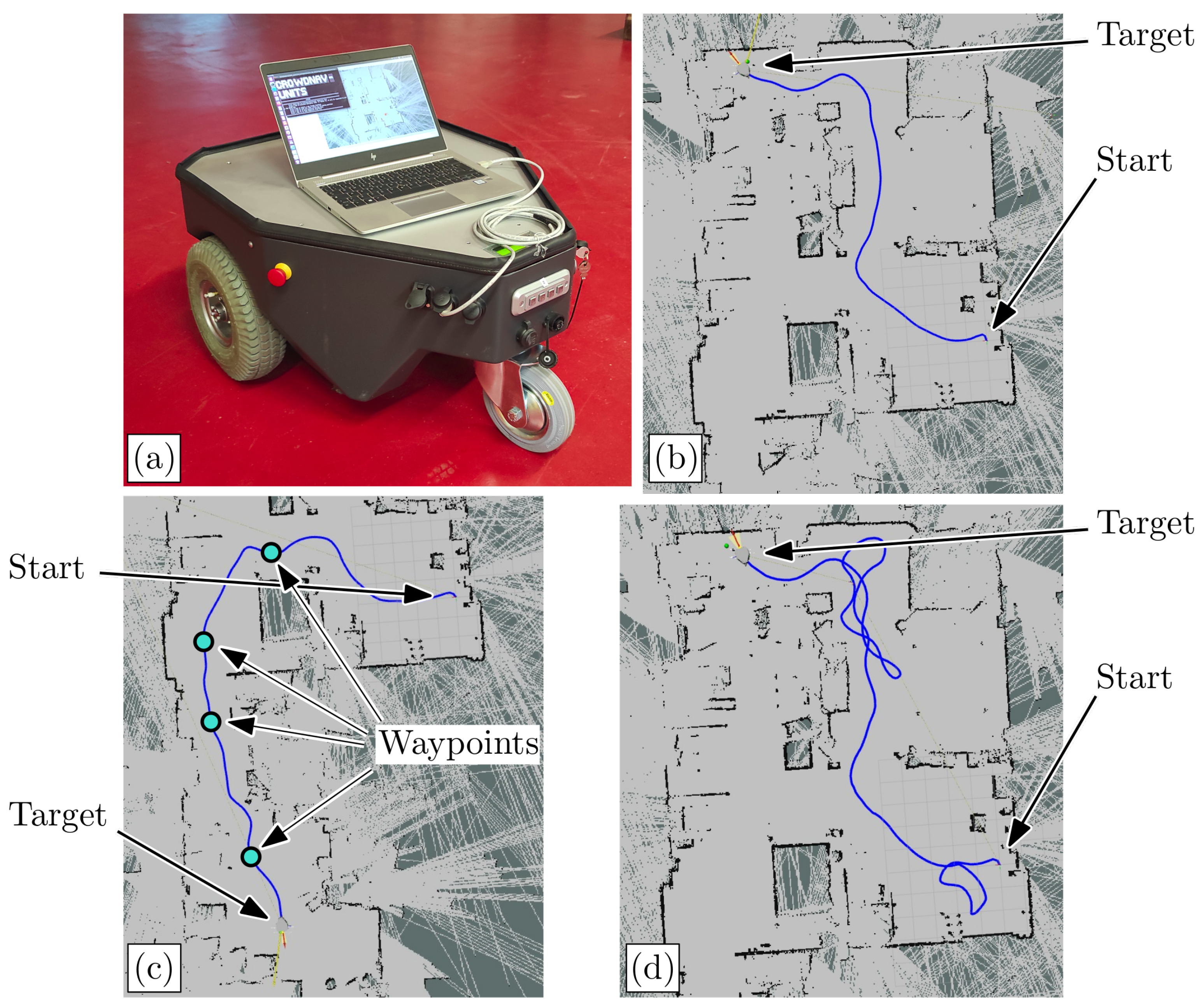
In order to carry out the test we used a Neobotix MP-500 robot (Neobotix GmbH, Hahnstrasse 2, Heilbronn, Germany), which is a ROS-Enabled differential drive mobile robot shown in Figure 15a. Perception is provided by a SICK S300 (SICK Vertriebs-GmbH, Willstaetterstrasse 30, Duesseldorf, Germany) bi-dimensional LiDAR Scanner, which is placed on the front side of the robot and provides the sensor readings needed by the NN. A dedicated ROS package has been developed for the purpose and has been tested prior to deployment in the Gazebo [40] dynamic simulation environment. The package mainly gathers sensor data and provides an interface for the NN to control the robot. Moreover, it implements the following additional functionalities: Simultaneous Localization and Mapping (SLAM), robots pose estimation, path planning, and user interaction. The ROS network is created in a way that ensures a master-slave configuration through the Ethernet, where the master is the laptop and the slave is the mobile robot. In this way a WiFi network is not required for the two devices to communicate, which allows for potentially unlimited operating range. The positioning of the robot in the environment is done combining two methods: (i) a dead reckoning technique (i.e., odometry) which was used to estimate the robot’s position by reading the wheels’ encoders, (ii) a probabilistic method that uses map knowledge and real-time readings from distance sensors. The combined information from both techniques allows for continuous correction of the poses of points of interest.

5.1. Case 1. Without Pedestrians

For this use case scenario, we test the system working both with point-to-point motions and through way-points. Specifically, the tests have been conducted in an indoor environment, i.e., the C6 laboratory of the University of Trieste.

In Figure 15b one can see the occupancy bi-dimensional map of part of the laboratory environment, obtained via ROS. The generated map shows the presence of many static obstacles; however, there are some obstacles that the LiDAR scanner was not able to detect. The figure refers to the test case for the point-to-point motion. In this case, the robot starts from the top left corner of the laboratory environment (indicated with the “START” label) and must reach the commanded target point (indicated with the “TARGET” label), which is placed at the bottom-right corner of the laboratory. The target point is chosen such that the robot is forced to negotiate with various obstacles, as well as to perform a 90 degrees turn and pass through a narrow corridor right before the target location. The blue line represents the trajectory that the mobile robot has followed, which shows that the robot has successfully performed the assigned point-to-point navigation and obstacle avoidance task. Moreover, the robot kept a safe distance from the obstacles.

In the waypoints test the robot is commanded to move along a longer path compared to that seen in the point-to-point test, as visible in Figure 15c. Together with the usual textboxes, the assigned way-points are indicated with the “WAYPOINTS” label, while the trajectory that the robot has performed is still shown as the blue curve. In the same figure, it can be noted that the robot has been assigned to a path through a very narrow corridor for most of its motion. However, similarly to the previous test, it can be seen that the robot has successfully performed the motion through way-points, avoiding the static obstacles that are present in the environment. Additionally, it has been noted that it is able to move in narrow corridors successfully.

5.2. Case 2. With Pedestrians

The location for this final experimental test is still the laboratory elected as an indoor testing environment. Conversely however, in this case, other than performing a point-to-point motion and avoiding static obstacles, the robot is required to avoid moving pedestrians that cross its path and move about in its close proximity. With reference to Figure 15d, the starting and target points assigned to the robot are the same ones used for the point-to-point motion test case described in the previous paragraph and indicated in green and red, respectively. The trajectory followed by the mobile robot during this point-to-point motion is again indicated with a blue curve.

The first detail one can notice in Figure 15d is that the curve representing the trajectory followed by the robot has tangles in some regions. This is because in these regions a moving pedestrian was in close proximity to the mobile robot, thus the latter had to perform some evasive maneuvers in order to avoid the former. It can be noted that despite the complexity introduced by moving pedestrians in the experimental environment, the mobile robot has still been able to avoid both static obstacles and pedestrians while at the same time moving up to the assigned target completely and safely without any collisions. The findings of this experimental testing also suggest that a simple bi-dimensional LiDAR scanner is able to detect the legs of pedestrians, and it is suitable for crowd navigation applications.

Finally, Figure 16 reports some video frames that have been extracted from the robot camera during its point-to-point motion. In some of the frames, the moving pedestrians can be seen crossing the mobile robot’s path and being in its close proximity.

6. Conclusions

In this work, we explored the development of a controller for a mobile robot capable of moving toward target locations, while at the same time avoiding both static and dynamic obstacles, e.g., pedestrians. The controller is based on a NN trained through two different RL algorithms: DQL and A3C. Our findings show that the A3C-trained NN performs better and generalizes the problem more effectively than the DQL-trained NN. Both algorithms are able to reach convergence, however, we show that the DQL-trained NN learns a sub-optimal strategy.

We leveraged the developed pipeline in order to run the NNs training in a highly parallelized environment, thus greatly cutting down the training time.

We applied this methodology to the use case of a complex dynamic environment with moving pedestrians. We have extended the ESFM to include realistic social behaviors of the simulated crowd in order to minimize the reality gap of the simulation. Using both trained NNs, the robot is able to complete the assigned task with a remarkable success ratio and at different pedestrian densities.

Additionally, the approach has also been tested experimentally, replicating the success of the simulations. Moreover, building from the raycasting approach used in the simulations, we showed that a bi-dimensional LiDAR scanner can be effectively used to detect pedestrians and thus provide meaningful data to the input of the NN. It must be pointed out that the test environment was not “robot friendly”, i.e., it presented many challenges for both the robot and its perception system.

Future work foresees an extension to not only consider bi-dimensional LiDAR sensors but also a robot equipped with a vision system. This will allow performing sensor fusion with the LiDAR readings, gaining more information about obstacles that are hardly manageable with just the bi-dimensional scanners. Moreover, the scenarios pool, with the simulated environment, will be further extended in order to include more critical scenarios such as mazes and narrow corridors. Furthermore, we will investigate the possibility to apply the findings of this research in training a controller for a more complex mobile robot such as those with four steerable wheels, in which each steering joint is subjected to joint limit constraints, as for instance the Archimede rover presented by Caruso et al. in Ref. [41].