Abstract
Highly three–dimensional and complex flow structures are closely related to the aerodynamic losses occurring in the transonic axial–flow compressor. The large eddy simulation (LES) approach was adopted to study the aerodynamic performance of the NASA rotor 37 for the cases at the design, the near stall (NS), and the near choke (NC) flow rate. The internal flow vortex topology was analyzed by the Q–criterion method, the omega (Ω) vortex identification method, and the Liutex identification method. It was observed that the Q–criterion method was vulnerable to being influenced by the flow with high–shear deformation rate, especially near the end–wall regions. The Ω method was adopted to recognize the three–dimensional vortex structure with a higher precision than that of the Q–criterion method. Meanwhile, the Liutex vortex identification method showed a good performance in vortex identification, and the corresponding contribution of Liutex components in the vortex topology was analyzed. The results show that the high–vortex fields around the separation line and reattachment line had high vortex components in the x–axis, the tip clearance vortices presented a high–vortex component in the y–axis, and the suction side corner vortex possessed high–vortex components in the y– and z–axes.
1. Introduction
For modern aero–engine design, the demands for low energy losses and high aerodynamic efficiency are always core challenges. A minor improvement in compressor performance can bring about considerable energy saving. Accurate recognition and understanding of the highly three–dimensional and complex flow structures inside a transonic rotor, which includes the different scale shedding vortices, is very helpful for the modern aero–engine design.
NASA has tested a series of transonic rotors and published the experimental data [1,2,3,4]. NASA rotor 37, a typical transonic rotor, was experimentally studied by NASA [2,3]. The experimental data were often used to testify various numerical codes [5,6,7] and were taken as the baseline model to investigate the aerodynamic phenomenon in transonic conditions [8,9]. Xue and Ge [8] studied the interaction between the shock and the tip leakage vortex in NASA rotor 37 and NASA rotor 67, finding that the vortex structure in the tip region possesses strong influences on rotor performance. Tang et al. [9] studied the influences of blade shapes on internal flow structures and proposed a blade tip redesign method that could reduce the tip vortex intensity and further improve the overall performance.
Knowledge of the flow structures in the transonic rotor has always fascinated researchers. The numerical approach provides a powerful method. Xiao and Cinnella [10] systematically evaluated the model uncertainty in Reynolds–averaged Navier–Stokes (RANS) simulations for the flow structures. They found that the RANS turbulence models could provide an acceptable accuracy in the evaluation of flow quantifications. By contrast, Charles [11] and Spalart et al. [12] studied the performance of detached eddy simulation (DES) and proposed that the numerical results predicated by using the DES approach were more reliable, especially for the fully developed turbulent flow. For the flow fields in transonic rotors, the numerical results of Hah et al. [13,14] demonstrated that the large eddy simulation (LES) method is superior to the DES and RANS methods in providing a more accurate internal flow structures, especially for the case at the near stall load.
The vortex structure has an evident influence on aerodynamic losses in the transonic axial compressors [15]. An appropriate method for describing the detailed internal flow structures and vortical topologies is important for us to understand the evolution of the flow characteristics. Different vortex identification approaches were proposed to study the internal vortex characteristics. Many typical approaches have been proposed, such as the three laws of Helmholtz [16], the Δ method [17], the Q–criterion method [18], the λcr method [19], and the λ2 method [20]. Recently, the Ω method [21,22,23] was suggested to discern the vortex structures. The Liutex identification method [24,25,26] was also suggested to recognize the vertical topology from another point of view. The aforementioned methods have found wide applications in the recognition of vortex topology of different physical models. For example, Bai et al. [27] conducted a comparative study of vortex identification methods in a tip–leakage cavitating flow and found that the Liutex method gave the best prediction. Wang et al. [28] performed the comparative study of the vortex recognition methods inside axial turbine rotor passages and drew a similar conclusion. Researchers have also conducted investigations on the vortex transient behaviors of sheet/cloud cavitating flow [29], vortex structures inside a miniature centrifugal pump [30,31], inlet vortices of an axial–flow pump [32], vortex identifications generated by the ship planar motion [33], and vortex flow in a gas cyclone [34]. However, a detailed study of the vortex topology inside the transonic compressor rotor is rare. Therefore, it is necessary to make a comparison and discussion of the feasibility of the vortex identification methods in a transonic compressor rotor by using the typical identification approaches.
This paper is organized as follows. The parameters of the NASA rotor 37 and the numerical model are presented in Section 2. A brief introduction of the Q–criterion, the Ω, and the Liutex identification method are presented in Section 3. In Section 4, the vortex structure and the vortex topology inside the rotor are studied systematically. Finally, conclusions are drawn in Section 5.
2. Physical Model and Numerical Model
2.1. Physical Model
NASA rotor 37 is a high–speed transonic turbofan that was designed by NASA and is used as the physical model to investigate the internal flow phenomenon inside a transonic turbomachine.
NASA rotor 37 has 36 blades and a design mass flow rate 20.188 kg/s. The rotor has an adiabatic efficiency of 0.877 and a total pressure ratio of 2.106. Its design rotating speed is 17,188.7 rpm. Radial distributions of the aerodynamic parameters were measured at stations 1 and 2, as shown in Figure 1. Axial station 1 is located at 4.19 cm ahead of the rotor leading edge (LE); meanwhile, axial station 2 is located at 10.67 cm downstream of the LE. Some parameters of the physical model are shown in Table 1.
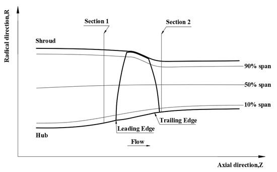
Figure 1.
NASA rotor 37 cross–section and span plane.

Table 1.
Parameters of the model.
2.2. Numerical Approach and Its Validation
The Reynolds–averaged Navier–Stokes equations are the governing equations for this flow:
The definitions of the variables are stated as follows: The symbol represents the flow density and is the time. The variable represents the velocity vector and denotes the pressure. The variable indicates the stress tensor and is the intrinsic enthalpy. Finally, the symbol represents the heat flux, is the gas constant number, and denotes the absolute temperature.
To enclose the governing equations, the turbulence model is adopted. The LES method was adopted to solve the equations. The Smagorinsky–type dynamic subgrid–scale (SGS) stress tensor was adopted to close the governing equations. The stress is expressed as
where is the Kronecker function, and and are the model coefficients.
The distributions of the grid and the y plus are shown in Figure 2. The structured mesh was produced with Turbogrid, and the CFD equations were solved with CFX. The inlet boundary of the computational domain locates two average blade heights ahead of the rotor LE. The outlet boundary locates three average blade heights downstream of the rotor trailing edge (TE). The average blade height is the blade height at the middle of the chord. For a single rotor passage, there are 380 nodes along the rotor streamwise direction, 62 nodes along the blade pitch direction, and 160 nodes along the blade height direction. More specifically, 90 from the 380 nodes are distributed inside the rotor blade in the streamwise direction, and 13 out of the 160 nodes are distributed in the clearance, which means a total of 13 layers are adopted in the tip clearance.
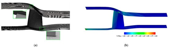
Figure 2.
Mesh generation and wall y plus. (a) Grid generation. (b) Grid wall y plus at design load.
It is generally suggested that y+ be less than 1 for LES simulations. As shown in Figure 2b, only in a few regions is the wall y+ value larger than 2, which basically meets the requirement of the LES numerical approach.
In the simulations, the ideal gas was adopted. On the inlet boundary, a reference total pressure was given as 101,325 Pa, and the inlet total temperature was given as 288.15 K. On the outlet boundary, different pressures were adopted to control the rotor operation condition. No–slip and adiabatic conditions were applied to the blade surface, the hub surface, and the shroud surface. The z–axis was selected as the axis of rotation of the rotor. A periodic interface was adopted for the two side surfaces of the single blade passage of the computational domain.
Total pressure ratio and adiabatic efficiency were chosen as the numerical approach validation characteristics, which are expressed as
where represents the total pressure at the inlet boundary, denotes the total pressure at the outlet boundary, is the rotor outlet adiabatic total enthalpy, is the rotor inlet total enthalpy, and denotes the rotor outlet total enthalpy.
Figure 3 provides the comparison of the experimental and numerical results of the performance of the transonic rotor. As shown in Figure 3, the LES results of the present investigation generally agree well with the LES results of Hah [13], and also match well with the experimental data, except at the choke condition. The errors between the simulated and the experimental data at the choke condition might have been due to the measurement uncertainty [13]. This comparison verified the present computational model.
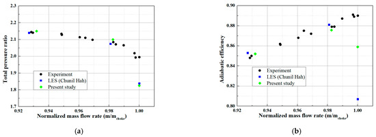
Figure 3.
Comparison of the numerical and experimental data of the rotor performance. (a) Total pressure ratio. (b) Adiabatic efficiency.
3. Vortex Identification Method Revisit
On the basis of Helmholtz decomposition [16], the vector can be expressed as the summation of an irrotational part and a solenoidal part. The movement of a fluid particle can be expressed as
More specifically, the vorticity tenser can be divided into a symmetric part and an anti–symmetric part, and Equation (11) can be simplified as the following equation:
where A denotes the symmetric part and B the anti–symmetric part. It is easy to find that A presents the particle deformation, and B is a term related to the whole vorticity intensity. For a specific flow condition, the variables a and b can be expressed as
3.1. Brief Introduction to the Q–Criterion Vortex Identification Method
The Q–criterion method was proposed by Hunt et al. [17]. In this method, the second Galilean invariant Q > 0 of the velocity gradient tensor is adopted to study the vortex structure. It is defined as
where the symbol denotes the Frobenius norm of the correspondence matrix.
For the Q–criterion method, only when the following two requirements are satisfied can the fields be considered as the rotation–dominated fields: (a) the value of function Q is positive, (b) the local pressure possesses the minimum value around the field. From Equation (16), it can be seen that the anti–symmetric B is required to be greater than the symmetric part A. To recognize the different scale vortices in the NASA rotor 37, the threshold value of is adopted as the vortex visualization criterion.
3.2. Brief Introduction to the Omega Vortex Identification Method
To find the intensity of vortical vorticity over the whole vorticity for a specific flow, the Ω method was suggested by Liu et al. [21,22,23]. The function of the approach is defined as
According to the correction made by Liu et al. [21,22,23], the function value Ω was modified as the following form:
where the parameter is a small number. The parameter is designed to avoid the condition of , and the is required to be a positive value. As Liu et al. [21,22,23] suggested, the in different cases have different values, and here the picks the approximate value of
where the variable amax denotes the maximum of a, and bmax denotes the maximum of b.
The Ω method is defined on the basis of the assumption that for an infinitesimal particle, the vortex is emerged for the flow with a strong vorticity part and a weak deformation part. Accordingly, the value of Ω is in the range of 0 ≤ Ω ≤ 1. For the cases of Ω > 0.5, it denotes the local field possess a vortex that is vorticity–dominant, and the local vorticity is greater than the deformation.
3.3. Brief Introduction to the Liutex Identification Method
To investigate the vortex structures and the vortex decomposition, the Liutex identification method was proposed by Liu et al. [24,25,26]. According to the definition, the rotating motion part of flow particles is extracted to represent the vortices. The real eigenvector of is adopted to denote the Liutex direction. The rotational strength is adopted to represent the Liutex magnitude. The function of Liutex is computed as
in a new XYZ–frame, where r is the real eigenvector of , and R denotes the local fluid particle rotation strength.
The Liutex is a vector with direction and magnitude, which can be used to represent the local fluid particle rotation. The Liutex direction is the local rotation axis, and the Liutex magnitude denotes the fluid rotational strength.
4. Discussion
4.1. Aerodynamic Performance of the NASA Rotor 37
Figure 4 provides the velocity fields at three spanwise locations of the transonic rotor at near stall (NS) condition, design condition, and near choke (NC) condition. At the NS condition, the velocity field was characterized by different–scale low–energy cells distributed upstream and downstream of the rotor, and there were no shock waves for the 10%, 50%, and 90% spans. At the design condition, the detached bow shock was captured at the 10%, 50%, and 90% spans. The detached bow shock was extended to the adjacent blade suction side in order to form a passage shock that further led to the suction side flow separation phenomenon. At the 90% span, the detached bow shock shown near the suction surface showed a λ shock pattern. The shock–boundary interaction phenomenon led to a large wake width after the blades. At the NC condition, the detached bow shock was much closer to the blade LE and its intensity clearly increased. At 50% span, a more severe flow separation occurred for the flow field near the blade suction surface. At the 90% span, the strong normal shock was located near the rotor TE. After the normal shock, the internal flow was gradually accelerated, and the secondary normal shock near the rotor blade trailing edge was captured.
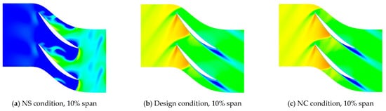
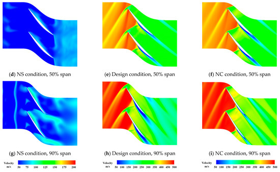
Figure 4.
Velocity fields of the NASA rotor 37 at NS condition (first column), design condition (second column) and NC condition (third column).
Figure 5 shows the suction side pressure maps and the limiting streamlines. To provide a quantitively analysis on the rotor flow separation phenomenon, the blade streamwise length was normalized with the rotor blade chord length c near the hub side, and the blade spanwise length was normalized with the rotor blade height along the rotor LE line. The detached line near the hub side moved downstream from the streamwise location 0.4c (NS condition) to the streamwise location 0.6c (NC condition). The streamwise length of the separation bubble increased with the incoming flow rate.
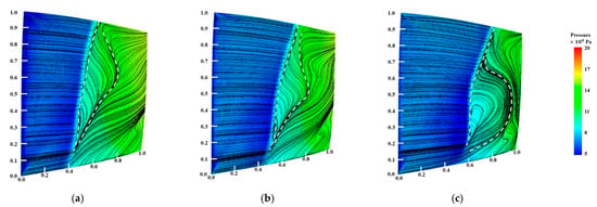
Figure 5.
Pressure maps and the limiting streamlines on the blade suction side at (a) NS condition, SS, (b) Design condition, SS, (c) NC condition, SS.
Figure 6 visualizes the relative velocity felids on the meridian plane of the rotor at the NS, design, and NC conditions. At the NS condition, vortices with different scales were observed clearly in the upstream rotor flow field and the downstream rotor field. A leakage jet existed at the rotor blade tip clearance. At the design condition, the tip leakage jet flow became strong; in the meantime, the vortices downstream of the blade were discerned, but the flow fields upstream of the blade showed many strips. The strips were the result of the bow shock waves. At the NC condition, a similar flow pattern appeared. However, the discrete vortices downstream of the blade became more evident, compared with those at design condition. The leakage jet flow had an increased velocity, and the interaction of the jet flow with the wake flow and the main flow became more evident.
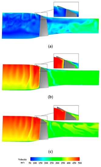
Figure 6.
Relative velocity fields on the meridian plane of the NASA rotor 37 at (a) NS condition, (b) design condition, (c) NC condition.
4.2. Vortex Structure Topology Analysis
Threshold values of the Q–criterion, the Ω, and the Liutex method were selected as below: (a) the threshold proposed by the theory authors, (b) the threshold used in the relevant studies, (c) thresholds by using the trial and error method. Following the relevant studies of vortex identification visualized by using the Q–criterion [27,30], the threshold value of function was adopted. The threshold function value of Ω = 0.52 was adopted following the suggestion of Liu et al. [23]. The threshold value was determined to be 1.7 × 10⁴ by trial and error for the Liutex method [24,25].
The vortex contours visualized by the Q–criterion identification method are presented in Figure 7. At the NS condition, different scale vortices in the upstream and downstream were visualized by the Q–criterion identification method. For the design and the NC cases, the tip clearance leakage vortices are clearly shown, and the downstream vortices are also identified.
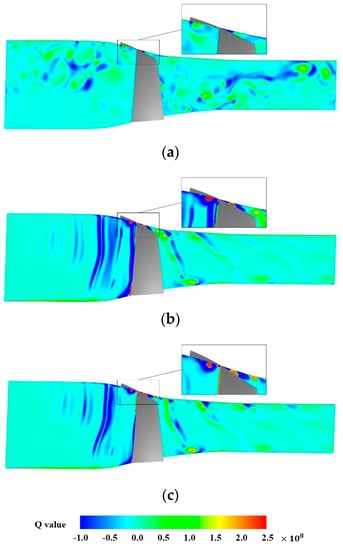
Figure 7.
Q value contours on the meridian plane of the NASA rotor 37 at (a) NS condition, (b) design condition, (c) NC condition.
Figure 8 shows the iso–surfaces of in a single blade passage at the three flow rates. The upstream and downstream vortices at different scales are clearly visualized by the iso–surface approach. Clearly, the regions with large Q values were mainly located near the shroud and hub surfaces and blade surfaces. It is somewhat strange that the flow at the end–walls in the blade upstream flow field also had high Q–values, although the incoming flow was uniform.
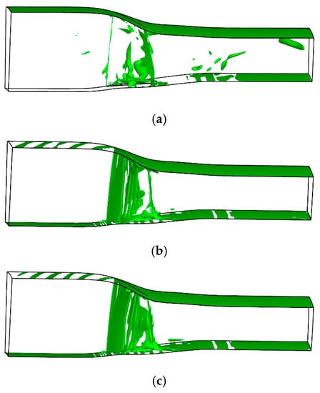
Figure 8.
Iso–surface of Q value in the NASA rotor 37 at (a) NS condition, (b) design condition, (c) NC condition.
The high Q value located in the end wall fields may be explained from its definition:
The stretching and compression of fluid particles (first three terms) as well as the shear deformation (last three terms) were considered in the Q–criterion identification method. The end–wall boundary layers had a high velocity gradient for the transonic rotor, which resulted in a high Q value.
Figure 9 demonstrates the detailed vortex contours visualized by the Ω method. Figure 10 further shows the three–dimensional vortices determined by the iso–surfaces of the value Ω in the rotor passage at the NS condition, design condition, and NC condition. Apparently, the vortex contours and the iso–surface results determined by the Q–criterion method and the Ω method were quite different. At the NS condition, many low–velocity vortices at different scales in the upstream/downstream of the rotor were seen when the internal flow field was analyzed by using the Ω method. Three–dimensional vortices visualized by the iso–surfaces of function Ω presented a similar distribution with those of the Q–criterion method, except for the vortex fields near the end–walls. This was because the function Ω is defined as a ratio of the fluid vorticity with the summation of the vorticity and the deformation rate of the fluid particle. Thus, the values of Ω in the boundary layer were not high and were unable to be shown if the iso–surface of function Ω = 0.52 was chosen. At the design condition, the three–dimensional vortices determined by the function Ω showed good agreement with the suction side separation line and reattachment line. Meanwhile, the vortices caused by the tip clearance leakage were well captured. At the NS condition, the downstream vorticity–dominated fields caused by the blade tip clearance leakage and the wake structures became strong.
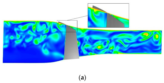
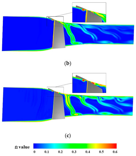
Figure 9.
Contour of Ω value of the NASA rotor 37 at (a) NS condition, (b) design condition, (c) NC condition.
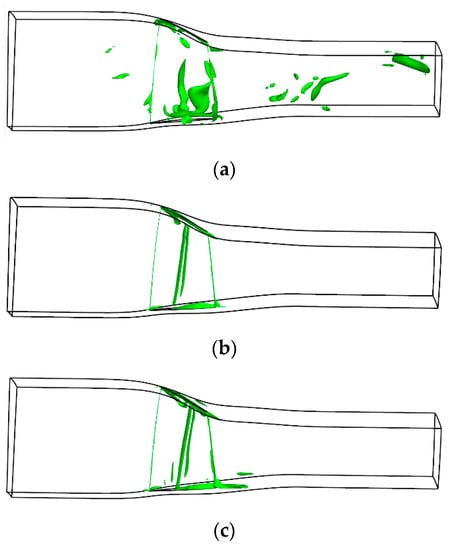
Figure 10.
Iso–surface of Ω value 0.52 in the NASA rotor 37 at (a) NS condition, (b) design condition, (c) NC condition.
Figure 11 presents the detailed vortex contour visualized by the Liutex identification method. Figure 12 provides the iso–surfaces of Liutex value with 1.7 × 10⁴ in the single passage at the NS, design, and NC conditions. The blade upstream and blade downstream vortices visualized by the Liutex showed good agreement with the local velocity fields (Figure 6). Unlike the vortex contour determined by the function Q and the function Ω, fields near the hub surface as well as the shroud surface had small Liutex values, and this was because the Liutex extracted the rotating motion part of flow particles to represent the vortices.
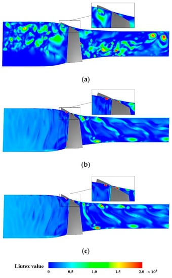
Figure 11.
Liutex value character in the NASA rotor 37 at (a) NS condition, (b) design condition, (c) NC condition.
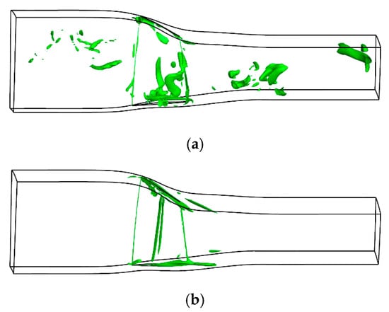
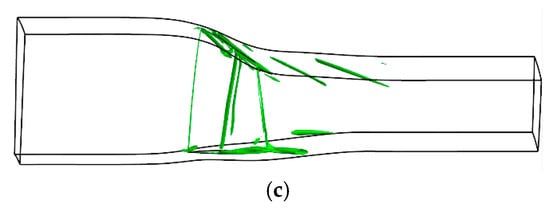
Figure 12.
Iso–surface of Liutex value 1.7 × 10⁴ in the NASA rotor 37 at (a) NS condition, (b) design condition, (c) NC condition.
The vorticity vector of the three–dimensional vortex structure was decomposed into vortex components in the x–, y–, and z–axes. Figure 13, Figure 14 and Figure 15 present the iso–surfaces of the three Liutex components at the NS, design, and the NC conditions, respectively.
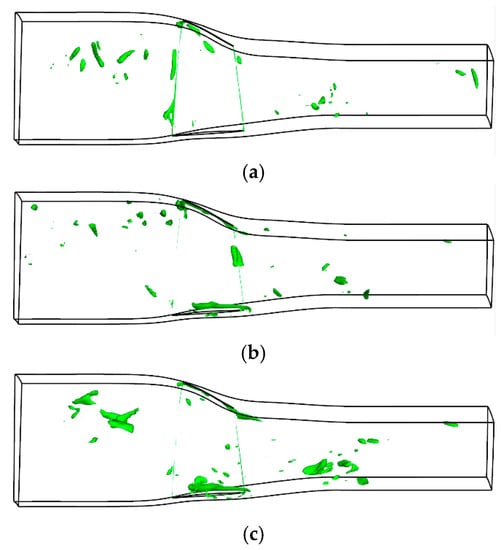
Figure 13.
Iso–surface of the Liutex components at the NS condition. (a) Liutex components in the x–axis. (b) Liutex components in the y–axis. (c) Liutex components in the z–axis.
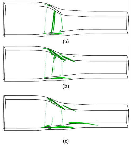
Figure 14.
Iso–surface of the Liutex components at the design condition. (a) Liutex component in the x–axis. (b) Liutex component in the y–axis. (c) Liutex component in the z–axis.
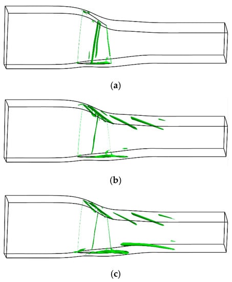
Figure 15.
Iso–surface of the Liutex components at the NC condition. (a) Liutex component in the x–axis. (b) Liutex component in the y–axis. (c) Liutex component in the z–axis.
At the NS condition, the rotor tip clearance vortices were mainly composed of the Liutex components in the y–axis and the z–axis. The upstream and downstream vortices shown in the rotor passage were mainly composed of the Liutex component in the z–axis. With the incoming flow rate increased to the design condition, the vorticity fields around the suction side separation line and reattachment line were captured by the Liutex method. The vortex topology results indicated that the high–vorticity fields around the suction side separation and reattachment lines were mainly composed of the Liutex component in the x–axis. The corner vortex near the suction side hub was mainly composed of the Liutex components in the y– and z–axes. Meanwhile, the tip clearance vortices had a high y–component. At the NC condition, the vortex fields around the separation line and reattachment line had a stronger vorticity intensity than those at the design condition. Vorticity intensities of the clearance vortex and the suction side corner vortex were also increased. The vortex decomposition results show that the Liutex components in the y– and z–axes were the main components of the rotor tip clearance vortices.
5. Conclusions
In this paper, the LES approach was adopted to investigate the transonic rotor flow characteristics at the NS, design, and NC conditions. The Q–criterion, the Ω, and the Liutex method were used to study the distribution and decomposition of the vortex structures in this transonic rotor in order to explore the occurrence and influence of the shedding vortices on the distortion and flow losses of the flow fields. Conclusions can be drawn as follows:
- (1)
- Comparison and discussion of the vortex structure in the NASA rotor 37 by using three typical vortex structure identification methods, namely, the Q–criterion, the Ω, and the Liutex method, were conducted. It was found that the Q–criterion method was vulnerable to being affected by the flow with high shear deformation rates, especially in the boundary layer, such as the end–wall fields of the NASA rotor 37, where the Q values are usually high.
- (2)
- Compared with the Q–criterion method, the Ω method is insensitive to the parameter threshold value and provides a way to visualize the three–dimensional vortex structures with a higher precision of vortex identification. However, the Ω method is a scalar field and cannot provide the direction of vortices, which are very useful in analyzing the flow fields and reducing the flow losses.
- (3)
- The Liutex identification method provides a vector parameter of R. Results show that the Liutex method shows high precision in the rotor vortex visualization. It was found that the high–vorticity fields around the separation line and reattachment line were mainly composed of the Liutex component in the x–axis, the tip clearance vortices had high Liutex components in the y–axis and z axis, and the suction side corner vortex was mainly composed of the Liutex components in the y–axis and the z–axis.
Author Contributions
Conceptualization, K.L. and P.T.; methodology, P.G. and J.L.; software, F.M.; validation, P.T.; formal analysis, K.L. and P.T.; data curation, F.M.; writing—original draft preparation, K.L. and P.T.; writing—review and editing, K.L., P.G. and J.L.; supervision, P.G. and J.L.; funding acquisition, J.L. All authors have read and agreed to the published version of the manuscript.
Funding
This work was financially supported by the National Science and Technology Major Project (2017–II–0007–0021) and the National Natural Science Foundation of China (51876158).
Data Availability Statement
Not applicable.
Conflicts of Interest
The authors declare no conflict of interest. The funders had no role in the design of the study; in the collection, analyses, or interpretation of data; in the writing of the manuscript; or in the decision to publish the results.
Nomenclature
| Symbols | |||
| A | particle deformation | P | pressure |
| a | particle deformation for a specific flow condition | P0 | total pressure |
| B | vorticity intensity | q | heat flux |
| b | vorticity intensity for a specific flow condition | Q | Q–criterion function value |
| c | rotor blade chord length near the hub side | R | gas constant number |
| E | intrinsic energy | t | time |
| H0 | total enthalpy | T | temperature |
| Ma | Mach number | Tpas | time spend for per passage |
| n | design rotating speed | u | velocity |
| N | number of blades | v | vorticity |
| Greek symbols | |||
| δij | Kronecker function | ρ | flow density |
| ε | correction factor | Ω | function in Ω method |
| η | adiabatic efficiency | τij | tress tensor |
| π | total pressure ratio | ||
| Subscripts | |||
| 1 | rotor inlet | NC | near choke |
| 2 | rotor outlet | NS | near stall |
| LE | blade leading–edge | TE | blade trailing–edge |
References
- Anthony, J.S.; Jerry, R.W.; Michael, D.H.; Suder, K.L. Laser anemometer measurements in a transonic axial-flow fan rotor. NASA Sti/Recon Tech. Rep. 1989, 90, 430–437. [Google Scholar]
- Reid, L.; Moore, R.D. Design and overall performance of four highly-loaded, high speed inlet stages for an advanced, high pressure ratio core compressor; NASA TP-1337; NASA: Washington, DC, USA, 1978.
- Reid, L.; Moore, R.D. Experimental study of low aspect ratio compressor blading. J. Eng. Gas Turbines Power 1980, 102, 875–882. [Google Scholar] [CrossRef]
- Reid, L.; Moore, R.D. Performance of a Single-Stage Axial-Flow Transonic Compressor with Rotor and Stator Aspect Ratios of 1.19 and 1.26, Respectively, and with Design Pressure Ratio of 1.82; NASA TP-1338; NASA: Washington, DC, USA, 1978.
- Hah, C.; Tsung, F.L.; Loellbach, J. Comparison of two three-dimensional unsteady Navier-Stokes codes applied to a turbine stage flow analysis. JSME Int. J. Ser. B 2008, 41, 200–207. [Google Scholar] [CrossRef]
- Cinnella, P.; Michel, B. Toward improved simulation tools for compressible turbomachinery: Assessment of residual-based compact schemes for the transonic compressor NASA Rotor 37. Int. J. Comput. Fluid Dyn. 2014, 28, 31–40. [Google Scholar] [CrossRef]
- Tiow, W.T.; Zangeneh, M. Application of a three-dimensional viscous transonic inverse method to NASA rotor 67. Proc. Inst. Mech. Eng. Part A J. Power Energy 2002, 216, 243–255. [Google Scholar] [CrossRef]
- Xue, Y.; Ge, N. Engineering application of an identification method to shock-induced vortex stability in the transonic axial fan rotor. Int. J. Aerosp. Eng. 2021, 31, 6611300. [Google Scholar] [CrossRef]
- Tang, X.; Luo, J.; Liu, F. Aerodynamic shape optimization of a transonic fan by an ad-joint-response surface method. Aerosp. Sci. Technol. 2017, 68, 26–36. [Google Scholar] [CrossRef]
- Xiao, H.; Cinnella, P. Quantification of model uncertainty in RANS simulations: A review. Prog. Aerosp. Sci. 2019, 108, 1–31. [Google Scholar] [CrossRef]
- Charles, M. A Comprehensive Study of Detached-Eddy Simulation; Technische Universität Berlin: Berlin, Germany, 2009. [Google Scholar]
- Spalart, P.R.; Jou, W.; Strelets, M.; Allmaras, S.R. Comments on the feasibility of LES for wings, and on a hybrid RANS/LES approach. Adv. DNS/LES 1997, 1997, 137–147. [Google Scholar]
- Hah, C. Large eddy simulation of transonic flow field in NASA Rotor 37. In Proceedings of the 47th AIAA Aerospace Sciences Meeting including the New Horizons Forum and Aerospace Exposition, Orlando, FL, USA, 5–8 January 2009. [Google Scholar] [CrossRef]
- Hah, C.; Wennerstrom, A.J. Three-dimensional flow fields inside a transonic compressor with swept blades. J. Turbomach. 1991, 113, 241–251. [Google Scholar] [CrossRef]
- Du, J.; Lin, F.; Chen, J.Y.; Nie, C.Q.; Biela, C. Flow structures in the tip region for a transonic compressor rotor. J. Turbomach. 2013, 135, 2561–2572. [Google Scholar] [CrossRef]
- Helmholtz, H. Über Integrale der hydrodynamischen Gleichungen, welche den Wirbelbewegungen entsprechen. J. Reine Angew. Math 1858, 55, 25–55. [Google Scholar]
- Chong, M.S.; Perry, A.E.; Cantwell, B.J. A general classification of three-dimensional flow fields. Phys. Fluids A Fluid Dyn. 1990, 2, 765–777. [Google Scholar] [CrossRef]
- Hunt, J.; Wray, A.; Moin, P. Eddies, Streams, and Convergence Zones in Turbulent Flows; In Center for Turbulence Research Report CTRS88; 1988; pp. 193–208. Available online: https://ntrs.nasa.gov/citations/19890015184 (accessed on 22 December 2022).
- Zhou, J.; Adrian, R.J.; Balachandar, S.; Kendall, T.M. Mechanisms for generating coherent packets of hairpin vortices in channel flow. J. Fluid Mach. 1999, 387, 353–396. [Google Scholar] [CrossRef]
- Jeong, J.; Hussain, F. On the identification of a vortex. J. Fluid Mech. 1995, 332, 339–363. [Google Scholar] [CrossRef]
- Liu, Z.N.; Liu, Z.X.; Liu, C.Q.; McCormick, S. Multilevel methods for temporal and spatial flow transition simulation in a rough channel. Int. J. Numer. Methods Fluids 2010, 19, 23–40. [Google Scholar] [CrossRef]
- Lu, P.; Yan, Y.H.; Liu, C.Q. Numerical investigation on mechanism of multiple vortex rings formation in late boundary-layer transition. Comput. Fluids 2013, 71, 156–168. [Google Scholar] [CrossRef]
- Liu, C.Q.; Wang, Y.Q.; Yang, Y.; Duan, Z.W. New omega vortex identification method. Sci. China Phys. Mech. Astron. 2016, 59, 684711. [Google Scholar] [CrossRef]
- Liu, C.Q.; Gao, Y.S.; Tian, S.L.; Dong, X.R. Rortex a new vortex vector definition and vorticity tensor and vector decompositions. Phys. Fluids 2018, 30, 035103. [Google Scholar] [CrossRef]
- Gao, Y.S.; Liu, C.Q. Rortex and comparison with eigenvalue-based vortex identification criteria. Phys. Fluids 2018, 30, 085107. [Google Scholar] [CrossRef]
- Liu, C.Q. Rortex based velocity gradient tensor decomposition. Phys. Fluids 2019, 31, 011704. [Google Scholar] [CrossRef]
- Bai, X.R.; Cheng, H.; Ji, B.; Long, X.; Peng, X. Comparative study of different vortex identification methods in a tip-leakage cavitating flow. Ocean Eng. 2020, 207, 107373. [Google Scholar] [CrossRef]
- Wang, Y.F.; Zhang, W.H.; Cao, X.; Yang, H.K. The applicability of vortex identification methods for complex vortex structures in axial turbine rotor passages. J. Hydrodyn. 2019, 31, 700–707. [Google Scholar] [CrossRef]
- Qu, S.H.; Li, J.P.; Cheng, H.Y.; Ji, B. LES investigation on vortex dynamics of transient sheet/cloud cavitating flow using different vortex identification methods. Mod. Phys. Lett. B 2020, 34, 2150111. [Google Scholar] [CrossRef]
- Li, K.H.; Chen, X.P.; Dou, H.S.; Zhu, Z.C.; Zheng, L.L.; Luo, X.W. Study of flow instability in a miniature centrifugal pump based on energy gradient method. J. Appl. Fluid Mech. 2019, 12, 701–713. [Google Scholar] [CrossRef]
- Li, K.H.; Xu, W.Q.; Dou, H.S. Flow stability in a miniature centrifugal pump under the periodic pulse flow. Energies 2021, 14, 8838. [Google Scholar] [CrossRef]
- Zhang, W.P.; Shi, L.J.; Tang, F.P.; Sun, Z.Z.; Zhang, Y. Identification and analysis of the inlet vortex of an axial-flow pump. J. Hydrodyn. 2022, 34, 234–243. [Google Scholar] [CrossRef]
- Ren, Z.; Wang, J.; Wan, D. Investigation of the flow field of a ship in planar motion mechanism tests by the vortex identification method. J. Mar. Sci. Eng. 2020, 8, 649. [Google Scholar] [CrossRef]
- Zhang, Z.H.; Dong, S.J.; Jin, R.Z.; Dong, K.J.; Hou, L.A.; Wang, B. Vortex characteristics of a gas cyclone determined with different vortex identification methods. Powder Technol. Int. J. Sci. Technol. Wet Dry Part. Syst. 2022, 404, 117370. [Google Scholar] [CrossRef]


Disclaimer/Publisher’s Note: The statements, opinions and data contained in all publications are solely those of the individual author(s) and contributor(s) and not of MDPI and/or the editor(s). MDPI and/or the editor(s) disclaim responsibility for any injury to people or property resulting from any ideas, methods, instructions or products referred to in the content. |
© 2023 by the authors. Licensee MDPI, Basel, Switzerland. This article is an open access article distributed under the terms and conditions of the Creative Commons Attribution (CC BY) license (https://creativecommons.org/licenses/by/4.0/).