Design and Stability Analysis of Sliding Mode Controller for Non-Holonomic Differential Drive Mobile Robots

Abstract

This paper presents a novel extended state observer (ESO) approach for a class of plants with nonlinear dynamics. The proposed observer estimates both the state variables and the total disturbance, which includes both exogenous and endogenous disturbance. The study’s changes can be summarized by developing a sliding mode higher-order extended state observer with a higher-order augmented state and a nonlinear function for the estimation error correction terms (SMHOESO). By including multiple enhanced states, the proposed observer can monitor total disturbances asymptotically, with the second derivative of the total disturbance serving as an upper constraint on the estimation error. This feature improves the observer’s ability to estimate higher-order disturbances and uncertainty. To extend the concept of the linear extended state observer (LESO), a nonlinear function can modify the estimation error in such a way that the proposed observer can provide faster and more accurate estimations of the state and total disturbance. The proposed nonlinearity also reduces the chattering issue with LESOs. This research thoroughly examines and analyzes the proposed SMHOESO’s convergence using the Lyapunov technique. According to this analysis, the SMHOESO is asymptotically stable, and the estimation error can be significantly reduced under real-world conditions. In addition to the SMHOESO, a modified Active Disturbance Rejection Control (ADRC) scheme is built, which includes a nonlinear state error feedback (NLSEF) controller and a nonlinear tracking differentiator (TD). Several nonlinear models, including the Differential Drive Mobile Robot (DDMR), are numerically simulated, and the proposed SMHOESO is compared to several alternative types, demonstrating a significant reduction in controller energy, increased control signal smoothness, and accurate tracking of the reference signal.

1. Introduction

As a result of unknown system dynamics or external perturbations, almost all physical systems in the real world have disturbances and uncertainties. Disturbance observers and related techniques are powerful tools for dynamically estimating, compensating, and controlling diverse disturbances in such systems [1]. This section describes the extended state observer (ESO), the disturbance observer (DOB), the perturbation observer (POB), and several other classes of approaches (ESO). The external disturbance is modelled as an enhanced state and estimated with a state observer in the Unknown Input Observer (UIO), one of the oldest disturbance estimators dating back to 1969 [2].

The DOB is another important class of disturbance estimators because it avoids using the plant’s nominal transfer function in some of its variants. DOB is based on the function’s inverse. Although POB and DOB are theoretically equivalent, POB is conceptualized in state space and designed in a discrete-time environment. UIO and DOB have been shown to be equally good at estimating disturbances, but UIO also provides state estimation [2].

An extended state observer (ESO) is used as a central component of Han’s active disturbance rejection control method and analyzes all internal and external disturbances [1]. As a result, it was possible to estimate both the extended state and the system state at the same time. Accurate uncertainty estimation contributes to improved disturbance rejection and a smooth control profile for the closed-loop system. Because an ESO can estimate internal uncertainties, the model’s required accuracy is reduced without compromising control performance [3]. Because of its convenience and high efficiency, the ESO is used in a wide range of industries, including robotics, aerospace, and electrical machines [1].

Throughout its rapid development in recent years, the ESO has been divided into two common types: linear ESO (LESO) and nonlinear ESO (NLESO). The LESO was developed as a backup option that also demonstrated the ease of tweaking parameters for theoretical analysis [4]. Significant gains may also result in peaking behavior, as seen in other high-gain observers [1,5,6,7]. The NLESO, on the other hand, was chosen in the early study due to its ability to effectively estimate nonlinear structures. Nonlinear ESO (NLESO) is created by feeding back the output estimation error using nonlinear functions. The nonlinear function is the mathematical fit of “big error, small gain” or “small error, big gain” and is usually chosen as a piecewise continuous, saturating, and monotonously increasing function. NLESO’s nonlinear gains are intended to reduce “peaking phenomenon” and to avoid large transient behaviors. A nonlinear observer is also used to ensure fast convergence and robustness against noise. Furthermore, because of its complex nonlinear features, proving the stability of a system using an NLESO is difficult. Han evaluated the convergence of the ESO estimation errors using the Lyapunov approach. Unfortunately, many assumptions were made in this study, and it can be difficult to find suitable nonlinear functions in practice. More generalized convergence results for single-input single-output (SISO) and multiple-input multiple-output (MIMO) systems have recently been discovered in [8,9], respectively.

Active Disturbance Rejection Control (ADRC) is becoming more popular as a technology, having been used successfully in engineering on numerous occasions. The recent implementation of ADRC technology at a Parker Hannifin Extrusion Plant in North America resulted in over 50% energy savings per line across 10 production lines, as well as significant improvements in product quality. Furthermore, thanks to the Kinetis^® motor suite’s simple interface and design approach, the field-oriented control (FOC) motor control design time cycle is reduced, system performance is increased, and support costs with ADRC are reduced [10]. It supports three-phase BLDC and PMSM motors via an algorithm with controls that are either low-cost but without sensors or very accurate with sensors. ADRC is used in [11] to evaluate the nonlinear kinematic model of the differential drive mobile robot (DDMR). Texas Instruments used ADRC technology in the development and global distribution of a new series of motion control chips (InstaSPINTM-MOTION). LineS-tream Technologies’ SpinTAC Motion Control Suite also includes an ADRC implementation. SpinTAC [12] is a Texas Instruments microcontroller (MCU) that uses InstaSPIN-MOTION technology. The National Superconducting Cyclotron Lab in the United States has used ADRC in several high-energy particle accelerators as a result of significant advances in the amplitude and phase regulation of electromagnetic fields [13].

This paper proposes a continuous nonlinear error function that is beneficial near the origin with limited large error values. A higher-order extended observer is also proposed, which allows an accurate estimation of high-order total disturbance. In this paper, a brief stability analysis is presented for both single-input single-output and multi-input multi-output systems.

This paper’s content is divided into six sections, with the related work outlined in Section 2. The proposed SMHOESO is described in Section 3, along with the relevant stability tests for single-input single-output systems, and the stability analysis for multi-input multi-output systems is covered in Section 4. Section 5 contains numerical simulations that confirm the accuracy of the proposed configuration, and Section 6 concludes.

2. Related Works

The LESO is similar to the Luenberger observer [14]. It is employed to simplify the calculation for an nth-order single-input-single-output system [9,15],

$$\left\{\begin{array}{c}{\dot{\xi }}_1\left(t\right)={\xi }_2\left(t\right), {\xi }_1\left(0\right)={\xi }_{10},\hfill \\ {\dot{\xi }}_2\left(t\right)={\xi }_3\left(t\right), {\xi }_2\left(0\right)={\xi }_{20},\hfill \\ \begin{array}{c}⋮\\ \begin{array}{c}{\dot{\xi }}_n\left(t\right)=f\left(t,{\xi }_1\left(t\right),{\xi }_2\left(t\right),\dots ,{\xi }_n\left(t\right)\right)+u\left(t\right)+w\left(t\right), {\xi }_n\left(t\right)={\xi }_{n0}\hfill \\ y\left(t\right)={\xi }_1\left(t\right)\hfill \end{array}\hfill \end{array}\end{array}\right.$$

(1)

where $\xi \left(0\right)=\left({\xi }_{10},{\xi }_{20},\dots ,{\xi }_{n0}\right)$ is the initial state, $\xi \left(t\right)=\left({\xi }_1\left(t\right),{\xi }_2\left(t\right),\dots ,{\xi }_n\left(t\right)\right)$ is the state vector of the system, $y(t)$ is the measured output, $f(.)\in C(R_n,R)$ is an unknown system function, $w(t)\in C(ℝ,ℝ)$ is the uncertain exogenous disturbance, $u(t)\in C(ℝ,ℝ)$ is the control input, $L(t)=f\left(t,.\right)+w(t)$ is denoted ‘‘total disturbance’’ [16]. By adding the extended state ${\xi }_{n+1}\left(t\right)\stackrel{\mathrm{def}}{=}f\left(t,.\right)+w(t)$, the system (1) can be restated as,

$$\left\{\begin{array}{c}{\dot{\xi }}_1\left(t\right)={\xi }_2\left(t\right), {\xi }_1\left(0\right)={\xi }_{10},\hfill \\ {\dot{\xi }}_2\left(t\right)={\xi }_3\left(t\right), {\xi }_2\left(0\right)={\xi }_{20},\hfill \\ \begin{array}{c}⋮\\ \begin{array}{c}\begin{array}{c}{\dot{\xi }}_n\left(t\right)={\xi }_{n+1}\left(t\right)+u\left(t\right), \xi \left(t\right)={\xi }_{n0}\hfill \\ {\dot{\xi }}_{n+1}\left(t\right)=\dot{f}\left(t,{\xi }_1\left(t\right),{\xi }_2\left(t\right),\dots ,{\xi }_n\left(t\right)\right)+\dot{w}\left(t\right), {\xi }_{n+1}\left(t\right)={\xi }_{n+\mathrm{1,0}},\hfill \end{array}\hfill \\ y\left(t\right)={\xi }_1\left(t\right)\hfill \end{array}\hfill \end{array}\end{array}\right.$$

(2)

A linear extended state observer [1],

$$\left\{\begin{array}{c}\begin{array}{c}{\dot{\widehat{\xi }}}_1\left(t\right)={\widehat{\xi }}_2\left(t\right)+{\beta }_1(y\left(t\right)-{\widehat{\xi }}_1\left(t\right)),\hfill \\ {\dot{\widehat{\xi }}}_2\left(t\right)={\widehat{\xi }}_3\left(t\right)+{\beta }_2(y\left(t\right)-{\widehat{\xi }}_1\left(t\right)),\hfill \end{array}\hfill \\ \begin{array}{c}⋮\\ {\dot{\widehat{\xi }}}_n\left(t\right)={\widehat{\xi }}_{n+1}(t)+u\left(t\right)+{\beta }_n(y\left(t\right)-{\widehat{\xi }}_1\left(t\right)),\hfill \\ {\dot{\widehat{\xi }}}_{n+1}\left(t\right)={\beta }_{n+1}\left(y\left(t\right)-{\widehat{\xi }}_1\left(t\right)\right),\hfill \end{array}\end{array}\right.$$

(3)

where ${\beta }_i=\frac{a_i}{{\epsilon }^i}$ is the observer coefficient to be designed, $i\in \left\{\mathrm{1,2},\dots ,n,n+1\right\}$.

There are two common techniques for LESO tuning: pole placement [17] and the bandwidth method [18]. If the ultimate goal is to limit the number of ESO parameters (i.e., only one ESO parameter should be selected or modified), the ESO coefficients can be expressed in terms of the ESO’s bandwidth [19]. Choosing a bandwidth that is too large will result in a decrease in estimation error within a reasonable bound [20]. To avoid this, the observer bandwidth is set to be lower than the frequency of the unmodeled dynamics but higher than the frequency of the disturbance [21]. The ESO, on the other hand, will perform worse if its bandwidth is set to a value that is either too low or too high. When the ESO and controller bandwidth are too large, strong tracking performance and external disturbance rejection are possible.

The negative effects of using a large bandwidth value include the following, measurement noise degrades output tracking and introduces chattering on the control signal [22]. Secondly, the transient response of the ESO is reduced because large bandwidth values result in high-gain observers [23]. Finally, some unmodeled high frequencies dynamics may be activated above a certain frequency, leading to inconsistency in the closed-loop system. The two main reasons that prevent the bandwidth from being expanded are regarded to be noise and sample rates. As a result, an estimator bandwidth that balances tracking performance with noise tolerance must be chosen. To outperform the LESO, the authors of [1] developed a new class of adaptive ESO (AESO) in which the observer bandwidth changes over time. The disadvantage of this method is that as the AESO order increases, parameter adjustment may become more difficult [1].

The small variable $\epsilon$ was set as in [24] to mitigate the peaking phenomenon brought on by various ESO initial values,

$$\frac{1}{\epsilon }=\left\{\begin{array}{c}\begin{array}{cc}100t^3& 0\le t\le 1\end{array}\\ \begin{array}{cc}100& t>1\end{array}\hfill \end{array}\right.$$

Optimization methods such as Bacterial Foraging Optimization (BFO), Particle Swarm Optimization (PSO), and Evolutionary Algorithms (EA) are used instead of manually adjusting the ESO parameters. Eventually, the ESO begins to estimate the states. As a result, aggregated disturbances have no effect, and the controller compensates for them in real-time [11]. The parameters of ESO were also determined using a non-dominated Sorting Genetic Algorithm (NSGA-II) [25].

The nonlinear gains of NLESO are designed to reduce such peak phenomenon, as well as to avoid large transient behaviours [26]. A nonlinear observer is also applied to guarantee fast-convergence and robustness with respect to the noise [27]. A general nonlinear ESO is given by [28],

$$\left\{\begin{array}{c}\begin{array}{c}{\dot{\widehat{\xi }}}_1\left(t\right)={\widehat{\xi }}_2\left(t\right)+g_1(y\left(t\right)-{\widehat{\xi }}_1\left(t\right)),\hfill \\ {\dot{\widehat{\xi }}}_2\left(t\right)={\widehat{\xi }}_3\left(t\right)+g_2(y\left(t\right)-{\widehat{\xi }}_1\left(t\right)),\hfill \\ ⋮\end{array}\hfill \\ \begin{array}{c}{\dot{\widehat{\xi }}}_n\left(t\right)={\widehat{\xi }}_{n+1}(t)+u\left(t\right)+g_n(y\left(t\right)-{\widehat{\xi }}_1\left(t\right)),\hfill \\ {\dot{\widehat{\xi }}}_{n+1}\left(t\right)=g_{n+1}\left(y\left(t\right)-{\widehat{\xi }}_1\left(t\right)\right).\hfill \end{array}\end{array}\right.$$

(4)

If nonlinear functions $g_i:ℝ\to ℝ,i\in \{\mathrm{1,2},\dots ,n+1\}$ were chosen, the state variables of the nonlinear system might track the state variables of the original system and the total disturbance $L(t)$. The mathematical representation of “high error, small gain or small error, big gain” is known as a nonlinear function $g_i(.)$ [29]. This function can be illustrated as follows [30,31,32,33,34], and is typically chosen as a nonlinear combination power function,

$$fal\left(e,\alpha ,\delta \right)=\left\{\begin{array}{c}\begin{array}{cc}\frac{e}{{\delta }^{\alpha -1}}\hfill & \left|e\right|\le \delta \hfill \end{array}\hfill \\ \begin{array}{cc}{\left|e\right|}^{\alpha }sgn(e)& \left|e\right|>\delta \end{array}\hfill \end{array}\right.$$

(5)

where $\delta$ is a small number that is used to express the length of the linear part. The function $fal\left(.\right)$ is a piecewise continuous, nonlinear, saturation, and monotonically increasing function. Studies have shown that when the value of δ is too small, it is still easy for the phenomenon of high-frequency chattering to appear. Conversely, when the value of $\delta$ is too large, there is still a chattering phenomenon owing to its non-smooth feature at the point e= $\delta$ [35]. When α = 0.75, the degree of linearity of $fal\left(.\right)$ function is best. Practically, the value of α is generally selected as α = 0.01 [28] in order to select the appropriate observer gains and $fal\left(.\right)$ function parameters.

In this case, a genetic algorithm (GA) is used to find better ESO parameters. Other effective optimization algorithms, on the other hand, may be good candidates for this purpose [33]. The function proposed in [28] eliminates non-smooth transitions between linear and nonlinear parts of the $fal\left(.\right)$ function. To allow it to be applicable under many different circumstances, this function is able to adjust the curve shape, the range, and the central location. On the other hand, the function in [36] is smoother, and the shape and center position of the function can be better controlled. The work suggested in [37] proposes a nonlinear function that not only has a nonlinear characteristic but is also very smooth. In particular, this function can be separately adjusted as the function in [28] to adapt to the practical application of different situations and requirements [37]. There are further nonlinear control laws proposed in [38,39,40,41,42].

3. Observer Design for SISO Systems

This section presents the nonlinear single-input single-output LESO and SMHOESO’s convergence analysis.

3.1. Linear Extended State Observer (LESO)

Firstly, some assumptions are required:

Assumption 1.

The function $f$ is continuously differentiable for all $\left(t,\xi \left(t\right)\right)\in ℝ\times {ℝ}^n$.

Assumption 2.

$w(t)$ and $\dot{w}(t)$ are bounded and $w(t)$ belongs to a known compact set $W\subset ℝ$.

Assumption 3.

There is a positive constant $M$ such that $\left|\Delta \left(t\right)\right|\le M$ for $t\ge 0.$

Assumption 4.

There exist constants ${\lambda }_1,and {\lambda }_2,$ and positive definite, continuously differentiable functions $V,W:{ℝ}^{n+1}\to {ℝ}^{+}$ such that:

$${\lambda }_1{‖y‖}^2\le V\left(y\right)\le {\lambda }_2{‖y‖}^2,W\left(y\right)={‖y‖}^2$$

(6)

$${\sum }_{i=1}^n\frac{\partial V_i}{\partial y_i}\left(y_i-a_i{y}_1\right)-\frac{\partial V}{\partial y_{n+1}}{a}_{n+1}{y}_1\le -W(y)$$

(7)

Theorem 1.

Assume that we have the ESO of (3) and the system presented in (2). Then,

(i)

$\underset{t\to \infty }{\lim }\left|{\xi }_i(t)-{\widehat{\xi }}_i(t)\right|=O\left(\frac{1}{{{\omega }_0}^{n+2-i}}\right)$

(ii)

$\underset{\begin{array}{c}t\to \infty \\ {\omega }_0\to \infty \end{array}}{\lim }\left|{\xi }_i(t)-{\widehat{\xi }}_i(t)\right|=0$

where ${\xi }_i(t)$, and ${\widehat{\xi }}_i(t)$ symbolize the solution of (2) and (3) correspondingly, $i\in \{\mathrm{1,2},\dots n+1\}$.

Proof. 

Set $e_i\left(t\right)={\xi }_i\left(t\right)-{\widehat{\xi }}_i(t)$, $i\in \{\mathrm{1,2},\dots n+1\}$. Then by subtracting (3) from (2),

$$\left\{\begin{array}{c}\begin{array}{c}{\dot{\xi }}_1\left(t\right)-{\dot{\widehat{\xi }}}_1\left(t\right)={\xi }_2\left(t\right)-\left({\widehat{\xi }}_2\left(t\right)+{\beta }_1(y\left(t\right)-{\widehat{\xi }}_1\left(t\right))\right)\hfill \\ {\dot{\xi }}_2\left(t\right)-{\dot{\widehat{\xi }}}_2\left(t\right)={\xi }_3\left(t\right)-\left({\widehat{\xi }}_3\left(t\right)+{\beta }_2(y\left(t\right)-{\widehat{\xi }}_1\left(t\right))\right)\hfill \\ ⋮\end{array}\hfill \\ \begin{array}{c}{\dot{\xi }}_n\left(t\right)-{\dot{\widehat{\xi }}}_n\left(t\right)={\xi }_{n+1}\left(t\right)+u\left(t\right)-\left({\widehat{\xi }}_{n+1}\left(t\right)+u\left(t\right)+{\beta }_n(y\left(t\right)-{\widehat{\xi }}_1\left(t\right))\right)\hfill \\ {\dot{\xi }}_{n+1}\left(t\right)-{\dot{\widehat{\xi }}}_{n+1}\left(t\right)=\Delta \left(t\right)-{\beta }_{n+1}(y\left(t\right)-{\widehat{\xi }}_1\left(t\right))\hfill \end{array}\end{array}\right.$$

The estimating error dynamics are demonstrated by a straightforward calculation to satisfy,

$$\left\{\begin{array}{c}\begin{array}{c}{\dot{e}}_1\left(t\right)=e_2\left(t\right)-{\beta }_{1}e\left(t\right)\hfill \\ {\dot{e}}_2\left(t\right)=e_3\left(t\right)-{\beta }_{2}e\left(t\right)\hfill \\ ⋮\end{array}\hfill \\ \begin{array}{c}{\dot{e}}_n\left(t\right)=e_{n+1}\left(t\right)-{\beta }_{n}e\left(t\right)\hfill \\ {\dot{e}}_{n+1}\left(t\right)=\Delta \left(t\right)-{\beta }_{n+1}e\left(t\right)\hfill \end{array}\end{array}\right.$$

(8)

Let ${\beta }_i=a_i{{\omega }_0}^i$, where $a_i$, $i\in \{\mathrm{1,2},\dots n+1\}$ are design parameters, and ${\omega }_0$ is the ESO bandwidth. The final form of (8) is,

$$\left\{\begin{array}{c}\begin{array}{c}{\dot{e}}_1\left(t\right)=e_2\left(t\right)-{\omega }_0{a}_1.e_1\left(t\right)\hfill \\ {\dot{e}}_2\left(t\right)=e_3\left(t\right)-{{\omega }_0}^2{a}_2{e}_1\left(t\right)\hfill \\ ⋮\end{array}\hfill \\ \begin{array}{c}{\dot{e}}_n\left(t\right)=e_{i,n+1}\left(t\right)-{{\omega }_0}^n{a}_n.e_1\left(t\right)\hfill \\ {\dot{e}}_{n+1}\left(t\right)=\Delta \left(t\right)-{{\omega }_0}^{n+1}{a}_{n+1}.e_1\left(t\right)\hfill \end{array}\end{array}\right.$$

(9)

Time scale (9) to get,

$$\left\{\begin{array}{c}\begin{array}{c}\frac{d{e}_1\left(\frac{t}{{\omega }_0}\right)}{d\frac{t}{{\omega }_0}}=e_2\left(\frac{t}{{\omega }_0}\right)-{\omega }_0{a}_1.e_1\left(\frac{t}{{\omega }_0}\right)\\ \frac{d{e}_2\left(\frac{t}{{\omega }_{i0}}\right)}{d\frac{t}{{\omega }_0}}=e_3\left(\frac{t}{{\omega }_0}\right)-{{\omega }_0}^2{a}_2.e_1\left(\frac{t}{{\omega }_0}\right)\\ ⋮\end{array}\hfill \\ \begin{array}{c}\frac{{de}_n\left(\frac{t}{{\omega }_{i0}}\right)}{d\frac{t}{{\omega }_0}}=e_{n+1}\left(\frac{t}{{\omega }_0}\right)-{{\omega }_0}^n{a}_n.e_1\left(\frac{t}{{\omega }_0}\right)\\ \frac{{de}_{n+1}\left(\frac{t}{{\omega }_{i0}}\right)}{d\frac{t}{{\omega }_0}}=\Delta -{{\omega }_0}^{n+1}{a}_{n+1}.e_1\left(\frac{t}{{\omega }_0}\right)\end{array}\end{array}\right.$$

(10)

Let

$${\eta }_i\left(t\right)={{\omega }_0}^{n+1-i}{e}_i(\frac{t}{{\omega }_0}), i\in \{\mathrm{1,2},\dots n+1\}$$

(11)

$$e_i\left(\frac{t}{{\omega }_0}\right)=\frac{1}{{{\omega }_0}^{n+1-i}}{\eta }_i\left(t\right)$$

(12)

Taking the derivative (11) with respect to t yields,

$$\frac{{d\eta }_i\left(t\right)}{dt}={{\omega }_0}^{n+1-i}\frac{{de}_i\left(\frac{t}{{\omega }_0}\right)}{d\frac{t}{{\omega }_0}}\frac{d(\frac{t}{{\omega }_0})}{dt}={{\omega }_{i0}}^{n-i}\frac{{de}_i\left(\frac{t}{{\omega }_0}\right)}{d\frac{t}{{\omega }_0}}$$

(13)

Then,

$$\frac{{de}_i\left(\frac{t}{{\omega }_0}\right)}{d\frac{t}{{\omega }_0}}=\frac{1}{{{\omega }_0}^{n-i}}\frac{{d\eta }_i\left(t\right)}{dt}$$

Both (12) and (13) are substituted in (10) and the result is,

$$\left\{\begin{array}{c}\begin{array}{c}\frac{1}{{{\omega }_0}^{n-1}}\frac{{d\eta }_1\left(t\right)}{dt}=\frac{1}{{{\omega }_0}^{n-1}}{\eta }_2\left(t\right)-{\omega }_0{a}_1.\frac{1}{{{\omega }_0}^n}{\eta }_1\left(t\right)\hfill \\ \frac{1}{{{\omega }_0}^{n-2}}\frac{{d\eta }_2\left(t\right)}{dt}=\frac{1}{{{\omega }_0}^{n-2}}{\eta }_3\left(t\right)-{{\omega }_0}^2{a}_2.\frac{1}{{{\omega }_0}^n}{\eta }_1\left(t\right)\hfill \\ ⋮\end{array}\\ \begin{array}{c}\frac{{d\eta }_n\left(t\right)}{dt}={\eta }_{in+1}\left(t\right)-{{\omega }_0}^n{a}_n.\frac{1}{{{\omega }_0}^n}{\eta }_i\left(t\right)\hfill \\ \frac{1}{{{\omega }_0}^{-1}}\frac{{d\eta }_{i,n+2}\left(t\right)}{dt}=\Delta -{{\omega }_0}^{n+1}{a}_{n+1}.\frac{1}{{{\omega }_0}^n}{\eta }_1\left(t\right)\hfill \end{array}\end{array}\right.$$

The time-scaled estimation error dynamics are,

$$\left\{\begin{array}{c}\begin{array}{c}\frac{{d\eta }_1\left(t\right)}{dt}={\eta }_2\left(t\right)-a_1.{\eta }_1\left(t\right)\hfill \\ \frac{{d\eta }_2\left(t\right)}{dt}={\eta }_{i,3}\left(t\right)-a_2.{\eta }_1\left(t\right)\hfill \\ ⋮\end{array}\hfill \\ \begin{array}{c}\frac{{d\eta }_n\left(t\right)}{dt}={\eta }_{in+1}\left(t\right)-a_{i,n}.{\eta }_i\left(t\right)\hfill \\ \frac{{d\eta }_{n+1}\left(t\right)}{dt}=\frac{\Delta }{{\omega }_0}-a_{n+1}.{\eta }_1\left(t\right)\hfill \end{array}\end{array}\right.$$

(14)

Using the solution of (14) as a guide, we can determine the derivative of $V\left(\eta \right)$ with respect to t,

$$\begin{array}{c}{\left.\dot{V}\left(\eta \right)\right|}_{along(14)}={\displaystyle \sum _{i=1}^{n+1}}\frac{\partial V\left(\eta \right)}{\partial {\eta }_i}{\dot{\eta }}_i(t)\\ ={\displaystyle \sum _{i=1}^{n+1}}\frac{\partial V\left(\eta \right)}{{\eta }_i}\left({\eta }_{i+1}\left(t\right)-a_i.{\eta }_1\left(t\right)\right)+\frac{\partial V\left(\eta \right)}{\partial {\eta }_{n+1}}\left(\frac{\Delta }{{\omega }_0}-a_{n+1}.{\eta }_1\left(t\right)\right)\end{array}$$

Then,

$${\left.\dot{V}\left(\eta \right)\right|}_{along(14)}=\sum _{i=1}^{n+1}\frac{\partial V\left(\eta \right)}{{\eta }_i}\left({\eta }_{i+1}\left(t\right)-a_i.{\eta }_1\left(t\right)\right)+\frac{\partial V\left(\eta \right)}{\partial {\eta }_{n+1}}\frac{\Delta }{{\omega }_0}-\frac{\partial V\left(\eta \right)}{\partial {\eta }_{n+1}}{a}_{n+1}.{\eta }_1\left(t\right)$$

from (9) of assumption 4,

$${\left.\dot{V}\left(\eta \right)\right|}_{along(14)}\le -W(\eta )+\frac{\partial V\left(\eta \right)}{\partial {\eta }_{n+1}}\frac{\Delta }{{\omega }_0}$$

Given Assumptions 3 and 4 assume the Lyapunov functions $V,W:{ℝ}^{n+1}\to {ℝ}^{+}$ defined by $V\left(\eta \right)=<P\eta ,\eta >$, where $\eta \in {ℝ}^{\rho +1}$ and $P$ is a symmetric positive definite matrix. Suppose (6) in Assumption 4 with ${{\lambda }_1=\lambda }_{min}(P)$ and ${\lambda }_2={\lambda }_{max}(P)$. Thus, when $\left(\eta \right)\le {\lambda }_{max}(P){‖\eta ‖}^2$ and $\left|\frac{\partial V}{{\partial \eta }_{\rho +1}}\right|\le ‖\frac{\partial V(\eta )}{\partial \eta }‖$, then $\left|\frac{\partial V}{{\partial \eta }_{\rho +1}}\right|\le {2\lambda }_{max}(P)‖\eta ‖$. Moreover, $V\left(\eta \right)\le {\lambda }_{max}\left(P\right){‖\eta ‖}^2={\lambda }_{max}\left(P\right)W(\eta )$. Thus, $-W\left(\eta \right)\le -\frac{V\left(\eta \right)}{{\lambda }_{ma\xi }\left(P\right)}$. Finally, because ${\lambda }_{min}(P){‖\eta ‖}^2\le V(\eta )$, this leads to $‖\eta ‖\le \sqrt{\frac{V(\eta )}{{\lambda }_{min}(P)}}$. As a result,

$${\dot{V}}_i\left({\eta }_i\right)\le -\frac{V(\eta )}{{\lambda }_{max}\left(P\right)}+\frac{M}{{\omega }_0}2{\lambda }_{max}(P)\frac{\sqrt{V_i(\eta )}}{\sqrt{{\lambda }_{min}\left(P\right)}}$$

Since,

$$\frac{d}{dt}\sqrt{V(\eta )}=\frac{1}{2}\frac{1}{\sqrt{V(\eta )}}\dot{V}\left(\eta \right),$$

Then,

$$\frac{d}{dt}\sqrt{V(\eta )}\le \frac{1}{2}\frac{1}{\sqrt{V(\eta )}}(-\frac{V(\eta )}{{\lambda }_{max}\left(P\right)}+\frac{M}{{\omega }_0}2{\lambda }_{max}(P)\frac{\sqrt{V(\eta )}}{\sqrt{{\lambda }_{min}\left(\eta \right)}})$$

$$\frac{d}{dt}\sqrt{V(\eta )}\le -\frac{\sqrt{V(\eta )}}{2{\lambda }_{max}\left(P\right)}+\frac{M}{{\omega }_0}\frac{{\lambda }_{max}\left(P\right)}{\sqrt{{\lambda }_{min}\left(P\right)}}$$

(15)

Solving the ordinary differential Equation (15) gives,

$$\sqrt{V(\eta )}\le \frac{2M{{\lambda }^2}_{max}\left(P\right)}{{\omega }_0\sqrt{{\lambda }_{min}\left(P\right)}}\left(1-e^{-\frac{t}{2{\lambda }_{max}\left(P\right)}}\right)+\sqrt{V(\eta (0))}{e}^{-\frac{t}{2{\lambda }_{max}\left(P\right)}}$$

Using $‖\eta ‖\le \sqrt{\frac{V(\eta )}{{\lambda }_{min}(P)}}$ one gets,

$$‖\eta (t)‖\le \sqrt{\frac{1}{{\lambda }_{min}\left(P\right)}}\left(\frac{2M{{\lambda }^2}_{max}\left(P\right)}{{\omega }_0\sqrt{{\lambda }_{min}\left(P\right)}}\left(1-e^{-\frac{t}{2{\lambda }_{max}\left(P\right)}}\right)+\sqrt{V(\eta (0))}{e}^{-\frac{t}{2{\lambda }_{max}\left(P\right)}}\right)$$

$$‖\eta (t)‖\le \frac{2M{{\lambda }^2}_{max}\left(P\right)}{{\omega }_0{\lambda }_{min}\left(P\right)}\left(1-e^{-\frac{t}{2{\lambda }_{max}\left(P\right)}}\right)+\sqrt{\frac{V(\eta (0))}{{\lambda }_{min}\left(P\right)}}{e}^{-\frac{t}{2{\lambda }_{max}\left(P\right)}}$$

(16)

Therefore, it follows from (16) that,

$$\left|{\xi }_i(t)-{\widehat{\xi }}_i(t)\right|=\frac{1}{{{\omega }_{i0}}^{n+1-i}}\left|{\eta }_i\left({\omega }_{0}t\right)\right|\Rightarrow \left|{\xi }_i(t)-{\widehat{\xi }}_i(t)\right|\le \frac{1}{{{\omega }_0}^{n+1-i}}‖\eta ({\omega }_{0}t)‖$$

Then, Sub. (16) in the above equation gives,

$$\left|{\xi }_i\left(t\right)-{\widehat{\xi }}_i\left(t\right)\right|\le \frac{1}{{{\omega }_0}^{n+1-i}}\left(\frac{2M{{\lambda }^2}_{max}\left(P\right)}{{\omega }_0{\lambda }_{min}\left(P\right)}\left(1-e^{-\frac{{\omega }_{0}t}{2{\lambda }_{max}\left(P\right)}}\right)+\sqrt{\frac{V(\eta (0))}{{\lambda }_{min}\left(P\right)}}{e}^{-\frac{{\omega }_{0}t}{2{\lambda }_{max}\left(P\right)}}\right)$$

Finally, $\underset{t\to \infty }{\lim }\left|{\xi }_i(t)-{\widehat{\xi }}_i(t)\right|=\frac{1}{{{\omega }_0}^{n+2-i}}\frac{2M{{\lambda }^2}_{max}\left(P\right)}{{\lambda }_{min}\left(P\right)}=O\left(\frac{1}{{{\omega }_0}^{n+2-i}}\right)$

$$\underset{\begin{array}{c}t\to \infty \\ {\omega }_0\to \infty \end{array}}{\lim }\left|{\xi }_i(t)-{\widehat{\xi }}_i(t)\right|$$

□

3.2. Sliding Mode Higher Order Extended State Observer (SMHOESO)

Starting again from the nonlinear system (1) and by adding the extended states ${\xi }_{n+1}\left(t\right)\stackrel{\mathrm{def}}{=}f\left(t,.\right)+w\left(t\right)$, ${\xi }_{n+2}\left(t\right)\stackrel{\mathrm{def}}{=}\dot{f}\left(t,.\right)+\dot{w}\left(t\right)$, it can be restated as,

$$\left\{\begin{array}{c}\begin{array}{c}{\dot{\xi }}_1\left(t\right)={\xi }_2\left(t\right)\hfill \\ {\dot{\xi }}_2\left(t\right)={\xi }_3\left(t\right)\hfill \\ ⋮\end{array}\hfill \\ \begin{array}{c}{\dot{\xi }}_n\left(t\right)={\xi }_{n+1}\left(t\right)+u\left(t\right)\hfill \\ \begin{array}{c}{\dot{\xi }}_{n+1}\left(t\right)={\xi }_{n+2}\left(t\right)\hfill \\ {\dot{\xi }}_{n+2}\left(t\right)=\Delta \left(t\right)\hfill \end{array}\hfill \end{array}\end{array}\right.$$

(17)

where $\Delta \left(t\right)=\ddot{f}\left(t,{\xi }_1\left(t\right),{\xi }_2\left(t\right),\dots ,{\xi }_n\left(t\right)\right)+\ddot{w}\left(t\right).$ In order to prove the convergence of SMHOESO, the following assumptions are needed.

Assumption 5.

$w(t)$, $\dot{w}(t)$ and $\ddot{w}\left(t\right)$ are bounded and $w(t)$ belongs to a known compact set $W\subset ℝ$.

Assumption 6.

There exist constants ${\lambda }_1,and {\lambda }_2,$ and positive definite, continuously differentiable functions $V,W:{ℝ}^{n+2}\to {ℝ}^{+}$ such that,

$${\lambda }_1{‖y‖}^2\le V\left(y\right)\le {\lambda }_2{‖y‖}^2,W\left(y\right)={‖y‖}^2$$

(18)

$${\sum }_{i=1}^{n+1}\frac{\partial V\left(y\right)}{y_i}\left(y_{i+1}\left(t\right)-a_{i}k\left(\frac{y_1\left(t\right)}{{{\omega }_0}^n}\right).y_1\left(t\right)\right)-\frac{\partial V\left(y\right)}{\partial y_{n+2}}{a}_{n+2}k\left(\frac{y_1\left(t\right)}{{{\omega }_0}^n}\right).y_1\left(t\right)\le -W(y)$$

(19)

The proposed nonlinear sliding mode higher-order extended state observer (SMHOESO) is described as,

$$\left\{\begin{array}{c}\begin{array}{c}{\dot{\widehat{\xi }}}_1\left(t\right)={\widehat{\xi }}_2\left(t\right)+{\beta }_1\mathcal{g}(y\left(t\right)-{\widehat{\xi }}_1\left(t\right)),\hfill \\ {\dot{\widehat{\xi }}}_2\left(t\right)={\widehat{\xi }}_3\left(t\right)+{\beta }_2\mathcal{g}(y\left(t\right)-{\widehat{\xi }}_1\left(t\right)),\hfill \\ ⋮\end{array}\hfill \\ \begin{array}{c}{\dot{\widehat{\xi }}}_n\left(t\right)={\widehat{\xi }}_{n+1}\left(t\right)+u\left(t\right)+{\beta }_n\mathcal{g}\left(y\left(t\right)-{\widehat{\xi }}_1\left(t\right)\right),\hfill \\ \begin{array}{c}{\dot{\widehat{\xi }}}_{n+1}\left(t\right)={\widehat{\xi }}_{n+1}(t)+{\beta }_{n+1}\mathcal{g}\left(y\left(t\right)-{\widehat{\xi }}_1\left(t\right)\right).\hfill \\ {\dot{\widehat{\xi }}}_{n+2}\left(t\right)={\beta }_{n+2}\mathcal{g}\left(y\left(t\right)-{\widehat{\xi }}_1\left(t\right)\right).\hfill \end{array}\hfill \end{array}\end{array}\right.$$

(20)

The mapping $\mathcal{g}:ℝ\to ℝ$ is selected as,

$$\mathcal{g}\left(e\right)=K_{\alpha }{\left|e\right|}^{\alpha }sign\left(e\right)+K_{\beta }{\left|e\right|}^{\beta }e$$

(21)

where $K_{\alpha },K_{\beta },\alpha and \beta$ are nonzero design coefficients (see Figure 1). Let ${\beta }_i=a_i{{\omega }_0}^i$, and rewrite (21) as $g_{proposed}(e)=\left(K_{\alpha }\frac{{\left|e\right|}^{\alpha }}{e}sign\left(e\right)+K_{\beta }{\left|e\right|}^{\beta }\right)e$. Then,

$$g_i\left(e\right)=\left\{\begin{array}{c}\begin{array}{cc}0& e=0\end{array}\hfill \\ \begin{array}{cc}k\left(e\right).e& e\ne 0\end{array}\hfill \end{array}\right.$$

(22)

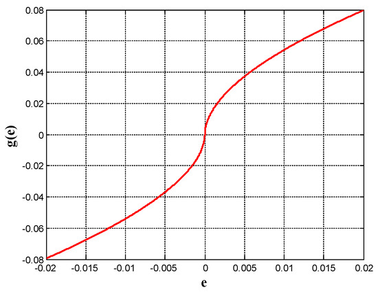
Figure 1. The function $\mathcal{g}$ with $\beta =0.334,\alpha =0.533,k_{\beta }=0.543,k_{\alpha }=0.617$.

The mapping $k:ℝ\to {ℝ}^{+}$is an odd nonlinear gain mapping with,

$$k\left(e\right){=K}_{\alpha }{\left|e\right|}^{\alpha -1}+K_{\beta }{\left|e\right|}^{\beta }$$

Lemma 1.

Assume that we have Lyapunov functions $V,W:{ℝ}^{n+2}\to {ℝ}^{+}$ expressed as $W\left(\eta \right)=V\left(\eta \right)=<P\eta ,\eta >$, where $\eta \in {ℝ}^{n+2}$ and $P$ is a symmetric and positive definite matrix. Suppose Assumption 6 Equation (18) with ${{\lambda }_1=\lambda }_{min}(P)$ and ${\lambda }_2={\lambda }_{max}(P)$. Then,

(i)

$\left|\frac{\partial V}{{\partial \eta }_{n+2}}\right|\le {2\lambda }_{max}(P)‖\eta ‖$

(ii)

$‖\eta ‖\le \sqrt{\frac{V(\eta )}{{\lambda }_{min}(P)}}$

(iii)

$-W(\eta )\le \frac{-V(\eta )}{max\left(P\right)}$

Proof. 

(i) Since $V\left(\eta \right)\le {\lambda }_{ma\xi }(P){‖\eta ‖}^2$ and $\left|\frac{\partial V}{{\partial \eta }_{n+2}}\right|\le ‖\frac{\partial V(\eta )}{\partial \eta }‖$, then, $\left|\frac{\partial V}{{\partial \eta }_{n+2}}\right|\le {2\lambda }_{max}(P)‖\eta ‖$. (ii) Since ${\lambda }_{min}(P){‖\eta ‖}^2\le V(\eta )$. This leads to $‖\eta ‖\le \sqrt{\frac{V(\eta )}{{\lambda }_{min}(P)}}$. Finally, (iii) Since $V\left(\eta \right)\le {\lambda }_{max}\left(P\right)W_i(\eta )$, then $V\left(\eta \right)\le {\lambda }_{max}\left(P\right)W_i(\eta )$ and $-W(\eta )\le \frac{-V\left(\eta \right)}{{\lambda }_{max}\left(P\right)}$. □

Theorem 2.

Assume that we have the plant of (2) and SMHOESO in (20). Then,

$$\underset{t\to \infty }{\lim }\left|{\xi }_i(t)-{\widehat{\xi }}_i(t)\right|=O\left(\frac{1}{{{\omega }_0}^{n+3-i}}\right)$$

where${\xi }_i(t)$, and${\widehat{\xi }}_i(t)$signify the solution of (2) and (20) correspondingly,$i\in \{\mathrm{1,2},\dots n+2\}$.

Proof. 

Set $e_i\left(t\right)={\xi }_i\left(t\right)-{\widehat{\xi }}_i(t)$, $i\in \{\mathrm{1,2},\dots n+2\}$. Then,

$$\left\{\begin{array}{c}\begin{array}{c}{\dot{\xi }}_1\left(t\right)-{\dot{\widehat{\xi }}}_1\left(t\right)={\xi }_2\left(t\right)-\left({\widehat{\xi }}_2\left(t\right)+{\beta }_1\mathcal{g}(y\left(t\right)-{\widehat{\xi }}_1\left(t\right))\right)\hfill \\ {\dot{\xi }}_2\left(t\right)-{\dot{\widehat{\xi }}}_2\left(t\right)={\xi }_3\left(t\right)-\left({\widehat{\xi }}_3\left(t\right)+{\beta }_2\mathcal{g}(y\left(t\right)-{\widehat{\xi }}_1\left(t\right))\right)\hfill \\ ⋮\end{array}\hfill \\ \begin{array}{c}{\dot{\xi }}_n\left(t\right)-{\dot{\widehat{\xi }}}_n\left(t\right)={\xi }_{n+1}\left(t\right)+u\left(t\right)-\left({\widehat{\xi }}_{n+1}\left(t\right)+u\left(t\right)+{\beta }_n\mathcal{g}(y\left(t\right)-{\widehat{\xi }}_1\left(t\right))\right)\hfill \\ {\dot{\xi }}_{n+1}\left(t\right)-{\dot{\widehat{\xi }}}_{n+1}\left(t\right)={\xi }_{n+2}\left(t\right)-\left({\widehat{\xi }}_{n+2}\left(t\right)+{\beta }_{n+1}\mathcal{g}(y\left(t\right)-{\widehat{\xi }}_1\left(t\right))\right)\hfill \\ {\dot{\xi }}_{n+2}\left(t\right)-{\dot{\widehat{\xi }}}_{n+2}\left(t\right)=\Delta \left(t\right)-{\beta }_{n+1}\mathcal{g}(y\left(t\right)-{\widehat{\xi }}_1\left(t\right))\hfill \end{array}\end{array}\right.$$

A simple calculation demonstrates that the estimating error dynamics meet,

$$\left\{\begin{array}{c}\begin{array}{c}{\dot{e}}_1\left(t\right)=e_2\left(t\right)-{\beta }_1\mathcal{g}\left(e_1\left(t\right)\right)\hfill \\ {\dot{e}}_2\left(t\right)=e_3\left(t\right)-{\beta }_2\mathcal{g}\left(e_1\left(t\right)\right)\hfill \\ ⋮\end{array}\hfill \\ \begin{array}{c}{\dot{e}}_n\left(t\right)=e_{n+1}\left(t\right)-{\beta }_n\mathcal{g}\left(e_1\left(t\right)\right)\hfill \\ {\dot{e}}_{n+1}\left(t\right)=e_{n+2}\left(t\right)-{\beta }_{n+1}\mathcal{g}\left(e_1\left(t\right)\right)\hfill \\ {\dot{e}}_{n+2}\left(t\right)=\Delta \left(t\right)-{\beta }_{n+2}\mathcal{g}\left(e_1\left(t\right)\right)\hfill \end{array}\hfill \end{array}\right.$$

(23)

The final form of (23) is,

$$\left\{\begin{array}{c}\begin{array}{c}{\dot{e}}_1\left(t\right)=e_2\left(t\right)-a_1{\omega }_{0}k\left(e_1\left(t\right)\right).e_1\left(t\right)\hfill \\ {\dot{e}}_2\left(t\right)=e_3\left(t\right)-a_2{{\omega }_0}^{2}k\left(e_1\left(t\right)\right).e_1\left(t\right)\hfill \\ ⋮\end{array}\hfill \\ \begin{array}{c}{\dot{e}}_n\left(t\right)=e_{n+1}\left(t\right)-a_n{{\omega }_0}^{n}k\left(e_1\left(t\right)\right).e_1\left(t\right)\hfill \\ {\dot{e}}_{n+1}\left(t\right)=e_{n+2}\left(t\right)-a_{n+1}{{\omega }_0}^{n+1}k\left(e_1\left(t\right)\right).e_1\left(t\right)\hfill \\ {\dot{e}}_{n+2}\left(t\right)=\Delta \left(t\right)-a_{n+2}{{\omega }_0}^{n+2}k\left(e_1\left(t\right)\right).e_1\left(t\right)\hfill \end{array}\hfill \end{array}\right.$$

(24)

Time scale (24) to get,

$$\left\{\begin{array}{c}\begin{array}{c}\frac{d{e}_1\left(\frac{t}{{\omega }_0}\right)}{d\frac{t}{{\omega }_0}}=e_2\left(\frac{t}{{\omega }_0}\right)-a_1{\omega }_{0}k\left(e_1\left(\frac{t}{{\omega }_0}\right)\right).e_1\left(\frac{t}{{\omega }_0}\right)\\ \frac{d{e}_2\left(\frac{t}{{\omega }_0}\right)}{d\frac{t}{{\omega }_0}}=e_3\left(\frac{t}{{\omega }_0}\right)-a_2{{\omega }_0}^{2}k\left(e_1\left(\frac{t}{{\omega }_0}\right)\right).e_1\left(\frac{t}{{\omega }_0}\right)\\ ⋮\end{array}\hfill \\ \begin{array}{c}\frac{d{e}_n\left(\frac{t}{{\omega }_0}\right)}{d\frac{t}{{\omega }_0}}=e_{n+1}\left(t\right)-a_n{{\omega }_0}^{n}k\left(e_1\left(\frac{t}{{\omega }_0}\right)\right).e_1\left(\frac{t}{{\omega }_0}\right)\hfill \\ \frac{d{e}_{n+1}\left(\frac{t}{{\omega }_0}\right)}{d\frac{t}{{\omega }_0}}=e_{n+2}\left(t\right)-a_{n+1}{{\omega }_0}^{n+1}k\left(e_1\left(\frac{t}{{\omega }_0}\right)\right).e_1\left(\frac{t}{{\omega }_0}\right)\hfill \\ \frac{d{e}_{n+2}\left(\frac{t}{{\omega }_0}\right)}{d\frac{t}{{\omega }_0}}=\Delta -a_{n+2}{{\omega }_0}^{n+2}k\left(e_1\left(\frac{t}{{\omega }_0}\right)\right).e_1\left(\frac{t}{{\omega }_0}\right)\hfill \end{array}\hfill \end{array}\right.$$

(25)

Let

$${\eta }_i\left(t\right)={{\omega }_0}^{n+1-i}{e}_{ij}(\frac{t}{{\omega }_0}), i\in \{\mathrm{1,2},\dots n+2\}$$

(26)

$$e_i\left(\frac{t}{{\omega }_0}\right)=\frac{1}{{{\omega }_{i0}}^{n+1-i}}{\eta }_i\left(t\right)$$

(27)

Taking the derivative (26) with respect to t yields,

$$\frac{{d\eta }_i\left(t\right)}{dt}={{\omega }_0}^{n+1-j}\frac{{de}_i\left(\frac{t}{{\omega }_0}\right)}{d(\frac{t}{{\omega }_0})}\frac{d(\frac{t}{{\omega }_0})}{dt}={{\omega }_0}^{n-i}\frac{{de}_i\left(\frac{t}{{\omega }_0}\right)}{d(\frac{t}{{\omega }_0})}$$

then,

$$\frac{{de}_i\left(\frac{t}{{\omega }_0}\right)}{d(\frac{t}{{\omega }_0})}={{\omega }_0}^{n-i}\frac{{d\eta }_i\left(t\right)}{dt}$$

(28)

Both (27) and (28) are substituted in (25) and the result is,

$$\left\{\begin{array}{c}\begin{array}{c}\frac{1}{{{\omega }_0}^{n-1}}\frac{{d\eta }_1\left(t\right)}{dt}=\frac{1}{{{\omega }_{i0}}^{n-1}}{\eta }_2\left(t\right)-{\omega }_0{a}_{1}k\left(\frac{{\eta }_1\left(t\right)}{{{\omega }_0}^n}\right).\frac{1}{{{\omega }_0}^n}{\eta }_1\left(t\right)\hfill \\ \frac{1}{{{\omega }_0}^{n-2}}\frac{{d\eta }_2\left(t\right)}{dt}=\frac{1}{{{\omega }_0}^{n-2}}{\eta }_3\left(t\right)-{{\omega }_0}^2{a}_{2}k\left(\frac{{\eta }_1\left(t\right)}{{{\omega }_0}^n}\right).\frac{1}{{{\omega }_0}^n}{\eta }_1\left(t\right)\hfill \\ ⋮\end{array}\hfill \\ \begin{array}{c}\frac{{d\eta }_n\left(t\right)}{dt}={\eta }_{n+1}\left(t\right)-{{\omega }_0}^n{a}_{n}k\left(\frac{{\eta }_1\left(t\right)}{{{\omega }_0}^n}\right).\frac{1}{{{\omega }_0}^n}{\eta }_1\left(t\right)\hfill \\ \frac{1}{{{\omega }_0}^{-1}}\frac{{d\eta }_{n+1}\left(t\right)}{dt}=\frac{1}{{{\omega }_0}^{-1}}{\eta }_{n+2}\left(t\right)-{{\omega }_0}^{n+1}{a}_{n+1}k\left(\frac{{\eta }_1\left(t\right)}{{{\omega }_0}^n}\right).\frac{1}{{{\omega }_0}^n}{\eta }_1\left(t\right)\hfill \\ \frac{1}{{{\omega }_0}^{-2}}\frac{{d\eta }_{n+2}\left(t\right)}{dt}=\Delta -{{\omega }_0}^{n+2}{a}_{n+2}k\left(\frac{{\eta }_1\left(t\right)}{{{\omega }_0}^n}\right).\frac{1}{{{\omega }_0}^n}{\eta }_1\left(t\right)\hfill \end{array}\end{array}\right.$$

The time-scaled estimation error dynamics are,

$$\left\{\begin{array}{c}\begin{array}{c}\frac{{d\eta }_1\left(t\right)}{dt}={\eta }_2\left(t\right)-a_{1}k\left(\frac{{\eta }_1\left(t\right)}{{{\omega }_0}^n}\right).{\eta }_1\left(t\right)\hfill \\ \frac{{d\eta }_2\left(t\right)}{dt}={\eta }_3\left(t\right)-a_{2}k\left(\frac{{\eta }_1\left(t\right)}{{{\omega }_0}^n}\right).{\eta }_1\left(t\right)\hfill \\ ⋮\end{array}\hfill \\ \begin{array}{c}\frac{{d\eta }_n\left(t\right)}{dt}={\eta }_{i,n+1}\left(t\right)-a_{n}k\left(\frac{{\eta }_1\left(t\right)}{{{\omega }_0}^n}\right).{\eta }_{i,j}\left(t\right)\\ \frac{{d\eta }_{n+1}\left(t\right)}{dt}={\eta }_{n+2}\left(t\right)-a_{n+1}k\left(\frac{{\eta }_1\left(t\right)}{{{\omega }_0}^n}\right).{\eta }_1\left(t\right)\\ \frac{{d\eta }_{n+2}\left(t\right)}{dt}=\frac{\Delta }{{{\omega }_0}^2}-a_{n+2}k\left(\frac{{\eta }_1\left(t\right)}{{{\omega }_0}^n}\right).{\eta }_1\left(t\right)\end{array}\hfill \end{array}\right.$$

(29)

Using the solution of Lemma 1 and finding the derivative of $V\left(\eta \right)$ with respect to t (29),

$${\left.\dot{V}\left(\eta \right)\right|}_{along(29)}=\sum _{i=1}^{n+2}\frac{\partial V\left(\eta \right)}{\partial {\eta }_i}{\dot{\eta }}_i(t)=\sum _{i=1}^{n+1}\frac{\partial V\left(\eta \right)}{{\eta }_i}\left({\eta }_{i+1}\left(t\right)-a_{i}k\left(\frac{{\eta }_1\left(t\right)}{{{\omega }_0}^n}\right).{\eta }_1\left(t\right)\right)+\frac{\partial V\left(\eta \right)}{\partial {\eta }_{n+2}}\left(\frac{\Delta }{{{\omega }_0}^2}-a_{n+2}k\left(\frac{{\eta }_1\left(t\right)}{{{\omega }_0}^n}\right).{\eta }_1\left(t\right)\right),$$

Then,

$${\left.\dot{V}\left(\eta \right)\right|}_{along(29)}=\sum _{i=1}^{n+1}\frac{\partial V\left(\eta \right)}{{\eta }_i}\left({\eta }_{i+1}\left(t\right)-a_{i}k\left(\frac{{\eta }_1\left(t\right)}{{{\omega }_0}^n}\right).{\eta }_1\left(t\right)\right)-\frac{\partial V\left(\eta \right)}{\partial {\eta }_{n+2}}{a}_{n+2}k\left(\frac{{\eta }_1\left(t\right)}{{{\omega }_0}^n}\right).{\eta }_1\left(t\right)+\frac{\partial V\left(\eta \right)}{\partial {\eta }_{n+2}}\frac{\Delta }{{{\omega }_0}^2}$$

from (19) of Assumption 6,

$${\left.\dot{V}\left(\eta \right)\right|}_{along(29)}\le -W(\eta )+\frac{\partial V\left(\eta \right)}{\partial {\eta }_{n+2}}\frac{\Delta }{{{\omega }_0}^2}$$

With the aid of Assumptions 2, 3 and 6 and the results of Lemma 1, it results in,

$${\dot{V}}_i\left({\eta }_i\right)\le -\frac{V(\eta )}{{\lambda }_{max}\left(P\right)}+\frac{M}{{{\omega }_0}^2}2{\lambda }_{max}(P)\frac{\sqrt{V_i(\eta )}}{\sqrt{{\lambda }_{min}\left(P\right)}}$$

Since,

$$\frac{d}{dt}\sqrt{V(\eta )}=\frac{1}{2}\frac{1}{\sqrt{V(\eta )}}\dot{V}\left(\eta \right)$$

Then,

$$\frac{d}{dt}\sqrt{V(\eta )}\le \frac{1}{2}\frac{1}{\sqrt{V(\eta )}}(-\frac{V(\eta )}{{\lambda }_{max}\left(P\right)}+\frac{M}{{{\omega }_0}^2}2{\lambda }_{max}(P)\frac{\sqrt{V(\eta )}}{\sqrt{{\lambda }_{min}\left(\eta \right)}})$$

$$\frac{d}{dt}\sqrt{V(\eta )}\le -\frac{\sqrt{V(\eta )}}{2{\lambda }_{max}\left(P\right)}+\frac{M}{{{\omega }_0}^2}\frac{{\lambda }_{max}\left(P\right)}{\sqrt{{\lambda }_{min}\left(P\right)}}$$

(30)

Solving the ordinary differential Equation (30) gives,

$$\sqrt{V(\eta )}\le \frac{2M{\lambda }_{max}^2\left(P\right)}{{{\omega }_0}^2\sqrt{{\lambda }_{min}\left(P\right)}}\left(1-e^{-\frac{t}{2{\lambda }_{ma\xi }\left(P\right)}}\right)+\sqrt{V(\eta (0))}{e}^{-\frac{t}{2{\lambda }_{max}\left(P\right)}}$$

$$‖\eta (t)‖\le \sqrt{\frac{1}{{\lambda }_{min}\left(P\right)}}\left(\frac{2M{{\lambda }^2}_{max}\left(P\right)}{{{\omega }_0}^2\sqrt{{\lambda }_{min}\left(P\right)}}\left(1-e^{-\frac{t}{2{\lambda }_{max}\left(P\right)}}\right)+\sqrt{V(\eta (0))}{e}^{-\frac{t}{2{\lambda }_{max}\left(P\right)}}\right)$$

$$‖\eta (t)‖\le \frac{2M{{\lambda }^2}_{max}\left(P\right)}{{{\omega }_0}^2{\lambda }_{min}\left(P\right)}\left(1-e^{-\frac{t}{2{\lambda }_{max}\left(P\right)}}\right)+\sqrt{\frac{V(\eta (0))}{{\lambda }_{min}\left(P\right)}}{e}^{-\frac{t}{2{\lambda }_{max}\left(P\right)}}$$

(31)

Therefore, it follows from (27) that,

$$\left|{\xi }_i(t)-{\widehat{\xi }}_i(t)\right|=\frac{1}{{{\omega }_{i0}}^{n+1-i}}\left|{\eta }_i\left({\omega }_{0}t\right)\right|\Rightarrow \left|{\xi }_i(t)-{\widehat{\xi }}_i(t)\right|\le \frac{1}{{{\omega }_0}^{n+1-i}}‖\eta ({\omega }_{0}t)‖$$

Then using (31) gives,

$$\left|{\xi }_i\left(t\right)-{\widehat{\xi }}_i\left(t\right)\right|\le \frac{1}{{{\omega }_0}^{n+1-i}}\left(\frac{2M{{\lambda }^2}_{max}\left(P\right)}{{{\omega }_0}^2{\lambda }_{min}\left(P\right)}\left(1-e^{-\frac{{\omega }_{0}t}{2{\lambda }_{max}\left(P\right)}}\right)+\sqrt{\frac{V(\eta (0))}{{\lambda }_{min}\left(P\right)}}{e}^{-\frac{{\omega }_{0}t}{2{\lambda }_{max}\left(P\right)}}\right)$$

Finally,

$$\underset{t\to \infty }{\lim }\left|{\xi }_i(t)-{\widehat{\xi }}_i(t)\right|=\frac{1}{{{\omega }_0}^{n+3-i}}\frac{2M{{\lambda }^2}_{max}\left(P\right)}{{\lambda }_{min}\left(P\right)}=O\left(\frac{1}{{{\omega }_0}^{n+3-i}}\right)$$

In the special case when the bandwidth of the SMHOESO goes very large, then,

$$\underset{\begin{array}{c}t\to \infty \\ {\omega }_0\to \infty \end{array}}{\lim }\left|{\xi }_i(t)-{\widehat{\xi }}_i(t)= 0 \right|$$

□

4. Observer Design for MIMO Systems

In this section, a class of MIMO systems with uncertainties and exogenous disturbances are considered as follows,

$$\left\{\begin{array}{c}\begin{array}{c}{\xi }_1^{(n)}\left(t\right)=f_1\left({t,\xi }_1\left(t\right),\dots ,{\xi }_1^{\left(n-1\right)}\left(t\right),\dots ,{\xi }_n^{\left(n-1\right)}\left(t\right)\right)+w_1\left(t\right)+\sum _{j=1}^n{b}_{1,j}{u}_j\left(t\right)\hfill \\ {\xi }_2^{(n)}\left(t\right)=f_2(t,{\xi }_1\left(t\right),\dots ,{\xi }_1^{(n-1)}\left(t\right),\dots ,{\xi }_n^{(n-1)}\left(t\right))+w_2\left(t\right)+\sum _{j=1}^n{b}_{2,j}{u}_j\left(t\right)\hfill \\ ⋮\end{array}\\ \begin{array}{c}{\xi }_n^{(n)}\left(t\right)=f_n({t,\xi }_1\left(t\right),\dots ,{\xi }_1^{(n-1)}\left(t\right),\dots ,{\xi }_n^{(n-1)}\left(t\right))+w_n\left(t\right)+\sum _{j=1}^n{b}_{n,j}{u}_j\left(t\right)\hfill \\ y_i\left(t\right)={\xi }_i\left(t\right)fori=\mathrm{1,2},\dots ,n\hfill \end{array}\end{array}\right.$$

(32)

where $u\left(t\right)={\left(u_1\left(t\right),u_2\left(t\right),\dots u_m\left(t\right)\right)}^T\in {ℝ}^n$ is the control input; $y\left(t\right)={\left(y_1\left(t\right),y_2\left(t\right),\dots y_m\left(t\right)\right)}^T\in {ℝ}^n$ is the output measured output; $f_i\in C({ℝ}^{+}\times {ℝ}^{n\times n},{ℝ}^n)$ an unknown system function for $i\in \{\mathrm{1,2},\dots n\}$; $w_i(t)\in C(ℝ,ℝ)$ the uncertain exogenous disturbance for $i\in \{\mathrm{1,2},\dots n\}$; and $\xi \left(t\right)=\left({\xi }_1\left(t\right),{\xi }_2\left(t\right),\dots ,{\xi }_n\left(t\right)\right)\in {ℝ}^n$ is the state vector of the system. A convenient way to represent the system (32) is,

$$\left(\begin{array}{c}\begin{array}{c}{\xi }_1^{(n)}\left(t\right)\\ {\xi }_2^{(n)}\left(t\right)\end{array}\\ \begin{array}{c}⋮\\ {\xi }_n^{(n)}\left(t\right)\end{array}\end{array}\right)=\left(\begin{array}{c}\begin{array}{c}{f}_1(.)\\ f_2(.)\end{array}\\ \begin{array}{c}⋮\\ f_n(.)\end{array}\end{array}\right)+\left(\begin{array}{c}\begin{array}{c}{w}_1\left(t\right)\\ w_2\left(t\right)\end{array}\\ \begin{array}{c}⋮\\ w_n\left(t\right)\end{array}\end{array}\right)+\left(\begin{array}{cc}\begin{array}{cc}{b}_{11}& b_{12}\\ b_{21}& b_{22}\end{array}& \begin{array}{cc}\dots & b_{1n}\\ \dots & b_{2n}\end{array}\\ \begin{array}{cc}⋮& ⋮\\ b_{n1}& b_{n2}\end{array}& \begin{array}{cc}\ddots & ⋮\\ \dots & b_{nn}\end{array}\end{array}\right)\left(\begin{array}{c}\begin{array}{c}{u}_1\left(t\right)\\ u_2\left(t\right)\end{array}\\ \begin{array}{c}⋮\\ u_n\left(t\right)\end{array}\end{array}\right)$$

(33)

For every $i,j\in \{\mathrm{1,2},\dots n\}$ there exists a constant $b_{i,j}$ such that the matrix $B$ with entry $b_{i,j}$ is invertible with inverse matrix given by,

$$\left(\begin{array}{ccc}{b}_{11}^{*}& \cdots & b_{1n}^{*}\\ ⋮& \ddots & ⋮\\ b_{n1}^{*}& \dots & b_{nn}^{*}\end{array}\right)={\left(\begin{array}{ccc}{b}_{11}& \cdots & b_{1n}\\ ⋮& \ddots & ⋮\\ b_{n1}& \dots & b_{nn}\end{array}\right)}^{-1}$$

(34)

Let the control inputs be denoted by,

$$\left(\begin{array}{c}\begin{array}{c}{u}_1\left(t\right)\\ u_2\left(t\right)\end{array}\\ \begin{array}{c}⋮\\ u_n\left(t\right)\end{array}\end{array}\right)=\left(\begin{array}{cc}\begin{array}{cc}{b}_{11}^{*}& b_{12}^{*}\\ b_{21}^{*}& b_{22}^{*}\end{array}& \begin{array}{cc}\dots & b_{1n}^{*}\\ \dots & b_{2n}^{*}\end{array}\\ \begin{array}{cc}⋮& ⋮\\ b_{n1}^{*}& b_{n2}^{*}\end{array}& \begin{array}{cc}\ddots & ⋮\\ \dots & b_{nn}^{*}\end{array}\end{array}\right)\left(\begin{array}{c}\begin{array}{c}{u}_1^{*}\left(t\right)\\ u_2^{*}\left(t\right)\end{array}\\ \begin{array}{c}⋮\\ u_n^{*}\left(t\right)\end{array}\end{array}\right)$$

(35)

Substitution of the control law (35) into the system (33) yields,

$$\left(\begin{array}{c}\begin{array}{c}{\xi }_1^{(n)}\left(t\right)\\ {\xi }_2^{(n)}\left(t\right)\end{array}\\ \begin{array}{c}⋮\\ {\xi }_n^{(n)}\left(t\right)\end{array}\end{array}\right)=\left(\begin{array}{c}\begin{array}{c}{f}_1(.)\\ f_2(.)\end{array}\\ \begin{array}{c}⋮\\ f_n(.)\end{array}\end{array}\right)+\left(\begin{array}{c}\begin{array}{c}{w}_1\left(t\right)\\ w_2\left(t\right)\end{array}\\ \begin{array}{c}⋮\\ w_n\left(t\right)\end{array}\end{array}\right)+\left(\begin{array}{cc}\begin{array}{cc}{b}_{11}& b_{12}\\ b_{21}& b_{22}\end{array}& \begin{array}{cc}\dots & b_{1n}\\ \dots & b_{2n}\end{array}\\ \begin{array}{cc}⋮& ⋮\\ b_{n1}& b_{n2}\end{array}& \begin{array}{cc}\ddots & ⋮\\ \dots & b_{nn}\end{array}\end{array}\right)\left(\begin{array}{cc}\begin{array}{cc}{b}_{11}^{*}& b_{12}^{*}\\ b_{21}^{*}& b_{22}^{*}\end{array}& \begin{array}{cc}\dots & b_{1n}^{*}\\ \dots & b_{2n}^{*}\end{array}\\ \begin{array}{cc}⋮& ⋮\\ b_{n1}^{*}& b_{n2}^{*}\end{array}& \begin{array}{cc}\ddots & ⋮\\ \dots & b_{nn}^{*}\end{array}\end{array}\right)\left(\begin{array}{c}\begin{array}{c}{u}_1^{*}\left(t\right)\\ u_2^{*}\left(t\right)\end{array}\\ \begin{array}{c}⋮\\ u_n^{*}\left(t\right)\end{array}\end{array}\right)$$

This with (34) gives,

$$\left(\begin{array}{c}\begin{array}{c}{\xi }_1^{(n)}\left(t\right)\\ {\xi }_2^{(n)}\left(t\right)\end{array}\\ \begin{array}{c}⋮\\ {\xi }_n^{(n)}\left(t\right)\end{array}\end{array}\right)=\left(\begin{array}{c}\begin{array}{c}{f}_1(.)\\ f_2(.)\end{array}\\ \begin{array}{c}⋮\\ f_n(.)\end{array}\end{array}\right)+\left(\begin{array}{c}\begin{array}{c}{w}_1\left(t\right)\\ w_2\left(t\right)\end{array}\\ \begin{array}{c}⋮\\ w_n\left(t\right)\end{array}\end{array}\right)+\left(\begin{array}{c}\begin{array}{c}{u}_1^{*}\left(t\right)\\ u_2^{*}\left(t\right)\end{array}\\ \begin{array}{c}⋮\\ u_n^{*}\left(t\right)\end{array}\end{array}\right)$$

(36)

Then, Equation (36) is transformed into a first-order system described by n number of subsystems of the first-order differential equations, where ${\xi }_{i,j}\left(t\right)={\xi }_i^{(j-1)}\left(t\right)for i,j\in \{\mathrm{1,2},\dots n\}$

$$\left\{\begin{array}{c}\begin{array}{c}{\dot{\xi }}_{i,1}\left(t\right)={\xi }_{i,2}\left(t\right)\hfill \\ {\dot{\xi }}_{i,2}\left(t\right)={\xi }_{i,3}\left(t\right)\hfill \\ ⋮\end{array}\hfill \\ \begin{array}{c}{\dot{\xi }}_{i,n}\left(t\right)=f_i\left({t,\xi }_{\mathrm{1,1}}\left(t\right),\dots ,{\xi }_{1,n}\left(t\right),\dots ,{\xi }_{n,n}\left(t\right)\right)+w_i\left(t\right)+u_i^{*}\left(t\right)\hfill \\ y_i\left(t\right)={\xi }_{i,1}\left(t\right)fori=\mathrm{1,2},\dots ,n\hfill \end{array}\end{array}\right.$$

(37)

By adding the extended states ${\xi }_{i,+1}\left(t\right)\stackrel{\mathrm{def}}{=}{f}_i\left(t,.\right)+w_i\left(t\right)$, ${\xi }_{i,n+2}\left(t\right)\stackrel{\mathrm{def}}{=}{\dot{f}}_i\left(t,.\right)+{\dot{w}}_i\left(t\right)$, the system (37) can be written as,

$$\left\{\begin{array}{c}\begin{array}{c}{\dot{\xi }}_{i,1}\left(t\right)={\xi }_{i,2}\left(t\right)\hfill \\ {\dot{\xi }}_{i,2}\left(t\right)={\xi }_{i,3}\left(t\right)\hfill \\ ⋮\end{array}\hfill \\ \begin{array}{c}{\dot{\xi }}_{i,n}\left(t\right)={\xi }_{i,n+1}\left(t\right)+u_i^{*}\left(t\right)\hfill \\ \begin{array}{c}{\dot{\xi }}_{i,n+1}\left(t\right)={\xi }_{i,n+2}\left(t\right)\hfill \\ {\dot{\xi }}_{i,n+2}\left(t\right)={\Delta }_i\left(t\right)\hfill \\ y_i\left(t\right)={\xi }_{i,1}\left(t\right)fori=\mathrm{1,2},\dots ,n\hfill \end{array}\hfill \end{array}\end{array}\right.$$

(38)

where ${\Delta }_i\left(t\right)={\ddot{f}}_i\left(t,{\xi }_1\left(t\right),{\xi }_2\left(t\right),\dots ,{\xi }_n\left(t\right)\right)+{\ddot{w}}_i\left(t\right)$. In order to prove the convergence of NLESO, the following definitions and assumptions are needed.

Definition 1.

A function ${\mathcal{g}}_i:ℝ\to ℝ$ is an odd nonlinear function with ${\mathcal{g}}_i\left(0\right)=0$. The nonlinear function ${\mathcal{g}}_i\left(.\right)$ is selected as follows:

$${\mathcal{g}}_i(e)=K_{i,\alpha }{\left|e\right|}^{{\alpha }_i}sign\left(e\right)+K_{i,\beta }{\left|e\right|}^{{\beta }_i}\left(e\right)$$

(39)

where$K_{i,\alpha },K_{i,\beta },{\alpha }_i,and {\beta }_i$are the positive design parameters. Rewriting (39) as,

$${\mathcal{g}}_i(e)=\left(K_{i,\alpha }\frac{{\left|e\right|}^{{\alpha }_i}}{e}sign\left(e\right)+K_{i,\beta }{\left|e\right|}^{{\beta }_i}\right)e$$

since sign($e$) =$e$/|$e$|, for$\left|e\right|\ne 0$, then,

$${\mathcal{g}}_i\left(e\right)=\left\{\begin{array}{c}\begin{array}{cc}0& e=0\end{array}\hfill \\ \begin{array}{cc}{k}_i\left(e\right).e& e\ne 0\end{array}\hfill \end{array}\right.$$

(40)

where,

$$k_i\left(e\right){=K}_{i,\alpha }{\left|e\right|}^{{\alpha }_i-1}+K_{i,\beta }{\left|e\right|}^{{\beta }_i}$$

(41)

The function  $k_i:ℝ\to {ℝ}^{+}$is a nonlinear gain function.

Assumption 7.

There exist continuous differentiable positive definite, functions $V_i,W_i:{ℝ}^{n+2}\to {ℝ}^{+}$ and constants ${\lambda }_{i,1},and {\lambda }_{i,2},$ such that:

$${\lambda }_{i,1}{‖y‖}^2\le V_i\left(y\right)\le {\lambda }_{i,2}{‖y‖}^2,W_i\left(y\right)={‖y‖}^2$$

(42)

$${\sum }_{j=1}^{n+1}\frac{\partial V_i}{\partial y_{i,j}}\left(y_{i,j+1}-a_{j}k\left(\frac{y_{i,1}\left(t\right)}{{{\omega }_0}^n}\right)y_{i,1}\right)-\frac{\partial V_i}{\partial y_{i,n+2}}{a}_{n+2}k\left(\frac{y_{i,1}\left(t\right)}{{{\omega }_0}^n}\right)y_{i,1}\le -W_i\left(y\right)$$

(43)

The following nonlinear higher-order extended state observer is proposed for the subsystem (37) with $i\in \{\mathrm{1,2},\dots n\}$.

$$\left\{\begin{array}{c}\begin{array}{c}{\dot{\widehat{\xi }}}_{i,1}\left(t\right)={\widehat{\xi }}_{i,2}\left(t\right)+{\beta }_{i,1}{\mathcal{g}}_i(y_i\left(t\right)-{\widehat{\xi }}_{i,1}\left(t\right))\hfill \\ {\dot{\widehat{\xi }}}_{i,2}\left(t\right)={\widehat{\xi }}_{i,3}\left(t\right)+{\beta }_{i,2}{\mathcal{g}}_i(y_i\left(t\right)-{\widehat{\xi }}_{i,1}\left(t\right))\\ ⋮\end{array}\hfill \\ \begin{array}{c}{\dot{\widehat{\xi }}}_{i,n}\left(t\right)={\widehat{\xi }}_{i,n+1}(t)+u_i^{*}\left(t\right)+{\beta }_{i,n}{\mathcal{g}}_i(y_i\left(t\right)-{\widehat{\xi }}_{i,1}\left(t\right))\hfill \\ {\dot{\widehat{\xi }}}_{i,n+1}\left(t\right)={\widehat{\xi }}_{i,n+2}\left(t\right)+{\beta }_{i,n+1}{\mathcal{g}}_i\left(y_i\left(t\right)-{\widehat{\xi }}_{i,1}\left(t\right)\right)\hfill \\ {\dot{\widehat{\xi }}}_{i,n+2}\left(t\right)={\beta }_{i,n+2}{\mathcal{g}}_i\left(y_i\left(t\right)-{\widehat{\xi }}_{i,1}\left(t\right)\right)\hfill \end{array}\hfill \end{array}\right.$$

(44)

Theorem 3.

Consider the system with augmented states given in (38), and the proposed nonlinear extended state observer (44). Then $\underset{t\to \infty }{\mathit{lim}}\left|{\xi }_{i,j}(t)-{\widehat{\xi }}_{i,j}(t)\right|=0$, where ${\xi }_{i,j}(t)$ and ${\widehat{\xi }}_{i,j}(t)$ represent the solution of (38) and (44), respectively, $i\in \{\mathrm{1,2},\dots n\},j\in \{\mathrm{1,2},\dots n+2\}$.

Proof. 

Set $e_{i,j}\left(t\right)={\xi }_{i,j}\left(t\right)-{\widehat{\xi }}_{i,j}(t)$, for $i\in \{\mathrm{1,2},\dots n\},j\in \{\mathrm{1,2},\dots n+2\}$. Then,

$$\left\{\begin{array}{c}\begin{array}{c}{\dot{\xi }}_{i,1}\left(t\right)-{\dot{\widehat{\xi }}}_{i,1}\left(t\right)={\xi }_{i,2}\left(t\right)-\left({\widehat{\xi }}_{i,2}\left(t\right)+{\beta }_{i,1}{\mathcal{g}}_i(y_i\left(t\right)-{\widehat{\xi }}_{i,1}\left(t\right))\right)\hfill \\ {\dot{\xi }}_{i,2}\left(t\right)-{\dot{\widehat{\xi }}}_{i,2}\left(t\right)={\xi }_{i,3}\left(t\right)-\left({\widehat{\xi }}_{i,3}\left(t\right)+{\beta }_{i,2}{\mathcal{g}}_i(y_i\left(t\right)-{\widehat{\xi }}_{i,1}\left(t\right))\right)\hfill \\ ⋮\end{array}\hfill \\ \begin{array}{c}{\dot{\xi }}_{i,n}\left(t\right)-{\dot{\widehat{\xi }}}_{i,n}\left(t\right)={\xi }_{i,n+1}\left(t\right)+u_i\left(t\right)-\left({\widehat{\xi }}_{i,n+1}\left(t\right)+u_i\left(t\right)+{\beta }_{i,n}{\mathcal{g}}_i(y_i\left(t\right)-{\widehat{\xi }}_{i,1}\left(t\right))\right)\hfill \\ {\dot{\xi }}_{i,n+1}\left(t\right)-{\dot{\widehat{\xi }}}_{i,n+1}\left(t\right)={\xi }_{i,n+2}\left(t\right)-\left({\widehat{\xi }}_{i,n+2}\left(t\right)+{\beta }_{i,n+1}{\mathcal{g}}_i(y_i\left(t\right)-{\widehat{\xi }}_{i,1}\left(t\right))\right)\hfill \\ {\dot{\xi }}_{i,n+2}\left(t\right)-{\dot{\widehat{\xi }}}_{i,n+2}\left(t\right)={\Delta }_i\left(t\right)-{\beta }_{i,n+1}{\mathcal{g}}_i(y_i\left(t\right)-{\widehat{\xi }}_{i,1}\left(t\right))\hfill \end{array}\hfill \end{array}\right.$$

A simple calculation demonstrates that the estimating error dynamics meet,

$$\left\{\begin{array}{c}\begin{array}{c}{\dot{e}}_{i,1}\left(t\right)=e_{i,2}\left(t\right)-{\beta }_{i,1}{\mathcal{g}}_i\left(e_{i,1}\left(t\right)\right)\hfill \\ {\dot{e}}_{i,2}\left(t\right)=e_{i,3}\left(t\right)-{\beta }_{i,2}{\mathcal{g}}_i\left(e_{i,1}\left(t\right)\right)\hfill \\ ⋮\end{array}\hfill \\ \begin{array}{c}{\dot{e}}_{i,n}\left(t\right)=e_{i,n+1}\left(t\right)-{\beta }_{i,n}{\mathcal{g}}_i\left(e_{i,1}\left(t\right)\right)\hfill \\ {\dot{e}}_{i,n+1}\left(t\right)=e_{i,n+2}\left(t\right)-{\beta }_{i,n+1}{\mathcal{g}}_i\left(e_{i,1}\left(t\right)\right)\hfill \\ {\dot{e}}_{i,n+2}\left(t\right)={\Delta }_i\left(t\right)-{\beta }_{i,n+2}{\mathcal{g}}_i\left(e_{i,1}\left(t\right)\right)\hfill \end{array}\hfill \end{array}\right.$$

(45)

Let ${\beta }_{i,j}=a_{i,j}{{\omega }_{i0}}^j$, where $a_{i,j}$, $i\in \{\mathrm{1,2},\dots n\},j\in \{\mathrm{1,2},\dots n+2\}$ are design parameters, and ${\omega }_0$ is the observer bandwidth. The estimation error dynamics (45) given that $g_i$ is represented by (40) and the final form is,

$$\left\{\begin{array}{c}\begin{array}{c}{\dot{e}}_{i,1}\left(t\right)=e_{i,2}\left(t\right)-{\omega }_{i0}{a}_{i,1}{k}_i\left(e_{i,1}\left(t\right)\right).e_{i,1}\left(t\right)\hfill \\ {\dot{e}}_{i,2}\left(t\right)=e_{i,3}\left(t\right)-{{\omega }_{i0}}^2{a}_{i,2}{k}_i\left(e_{i,1}\left(t\right)\right).e_{i,1}\left(t\right)\hfill \\ ⋮\end{array}\hfill \\ \begin{array}{c}{\dot{e}}_{i,n}\left(t\right)=e_{i,n+1}\left(t\right)-{{\omega }_{i0}}^n{a}_{i,n}{k}_i\left(e_{i,1}\left(t\right)\right).e_{i,1}\left(t\right)\hfill \\ {\dot{e}}_{i,n+1}\left(t\right)=e_{i,n+2}\left(t\right)-{{\omega }_{i0}}^{n+1}{a}_{i,n+1}{k}_i\left(e_{i,1}\left(t\right)\right).e_{i,1}\left(t\right)\hfill \\ {\dot{e}}_{i,n+2}\left(t\right)={\Delta }_i-{{\omega }_{i0}}^{n+2}{a}_{i,n+2}{k}_i\left(e_{i,1}\left(t\right)\right).e_{i,1}\left(t\right)\hfill \end{array}\hfill \end{array}\right.$$

(46)

Time scale (46) to get,

$$\left\{\begin{array}{c}\begin{array}{c}\frac{d{e}_{i,1}\left(\frac{t}{{\omega }_{i0}}\right)}{d\frac{t}{{\omega }_{i0}}}=e_{i,2}\left(\frac{t}{{\omega }_{i0}}\right)-{\omega }_{i0}{a}_{i,1}{k}_i\left(e_{i,1}\left(\frac{t}{{\omega }_{i0}}\right)\right).e_{i,1}\left(\frac{t}{{\omega }_{i0}}\right)\hfill \\ \frac{d{e}_{i,2}\left(\frac{t}{{\omega }_{i0}}\right)}{d\frac{t}{{\omega }_{i0}}}=e_{i,3}\left(\frac{t}{{\omega }_{i0}}\right)-{{\omega }_{i0}}^2{a}_{i,2}{k}_i\left(e_{i,1}\left(\frac{t}{{\omega }_{i0}}\right)\right).e_{i,1}\left(\frac{t}{{\omega }_{i0}}\right)\hfill \\ ⋮\end{array}\hfill \\ \begin{array}{c}\frac{{de}_{i,n}\left(\frac{t}{{\omega }_{i0}}\right)}{d\frac{t}{{\omega }_{i0}}}=e_{i,n+1}\left(\frac{t}{{\omega }_{i0}}\right)-{{\omega }_{i0}}^n{a}_{i,n}{k}_i\left(e_{i,1}\left(\frac{t}{{\omega }_{i0}}\right)\right).e_{i,1}\left(\frac{t}{{\omega }_{i0}}\right)\hfill \\ \frac{{de}_{i,n+1}\left(s\right)}{ds}=e_{i,n+2}\left(\frac{t}{{\omega }_{i0}}\right)-{{\omega }_{i0}}^{n+1}{a}_{i,n+1}{k}_i\left(e_{i,1}\left(\frac{t}{{\omega }_{i0}}\right)\right).e_{i,1}\left(\frac{t}{{\omega }_{i0}}\right)\hfill \\ \frac{{de}_{i,n+1}\left(\frac{t}{{\omega }_{i0}}\right)}{d\frac{t}{{\omega }_{i0}}}={\Delta }_i-{{\omega }_{i0}}^{n+2}{a}_{i,n+2}{k}_i\left(e_{i,1}\left(\frac{t}{{\omega }_{i0}}\right)\right).e_{i,1}\left(\frac{t}{{\omega }_{i0}}\right)\hfill \end{array}\hfill \end{array}\right.$$

(47)

Let ${\eta }_{i,j}\left(t\right)={{\omega }_{i,0}}^{n+1-j}{e}_{i,j}(\frac{t}{{\omega }_{i0}})$, $i\in \{\mathrm{1,2},\dots n\},j\in \{\mathrm{1,2},\dots n+2\}$, then,

$${\eta }_{i,j}\left(t\right)={{\omega }_{i0}}^{n+1-j}{e}_{i,j}\left(\frac{t}{{\omega }_{i0}}\right)\Rightarrow e_{i,j}\left(\frac{t}{{\omega }_{i0}}\right)=\frac{1}{{{\omega }_{i0}}^{n+1-j}}{\eta }_{i,j}\left(t\right)$$

(48)

Taking the derivative (48) with respect to s yields,

$$\begin{gathered} \frac{{d\eta }_{i,j}\left(t\right)}{dt}={{\omega }_{i0}}^{n+1-j}\frac{{de}_{i,j}\left(\frac{t}{{\omega }_{i0}}\right)}{d(\frac{t}{{\omega }_{i0}})}\frac{d(\frac{t}{{\omega }_{i0}})}{dt}={{\omega }_{i0}}^{n-j}\frac{{de}_{i,j}\left(\frac{t}{{\omega }_{i0}}\right)}{d(\frac{t}{{\omega }_{i0}})} \\ \frac{{de}_{i,j}\left(\frac{t}{{\omega }_{i0}}\right)}{d\frac{t}{{\omega }_{i0}}}=\frac{1}{{{\omega }_{i0}}^{n-j}}\frac{{d\eta }_{i,j}\left(t\right)}{dt} \end{gathered}$$

(49)

Both (48) and (49) are substituted in (47) and the result is,

$$\left\{\begin{array}{c}\begin{array}{c}\frac{1}{{{\omega }_{i0}}^{n-1}}\frac{{d\eta }_{i,1}\left(t\right)}{dt}=\frac{1}{{{\omega }_{i0}}^{n-1}}{\eta }_{i,2}\left(t\right)-{\omega }_{i0}{a}_{i,1}{k}_i\left(e_{i,1}\left(s\right)\right).\frac{1}{{{\omega }_{i0}}^n}{\eta }_{i,1}\left(t\right)\hfill \\ \frac{1}{{{\omega }_{i,0}}^{n-2}}\frac{{d\eta }_{i,2}\left(t\right)}{dt}=\frac{1}{{{\omega }_{i,0}}^{n-2}}{\eta }_{i,3}\left(t\right)-{{\omega }_{i0}}^2{a}_{i,2}{k}_i\left(e_{i,1}\left(s\right)\right).\frac{1}{{{\omega }_{i0}}^n}{\eta }_{i,1}\left(t\right)\hfill \\ ⋮\end{array}\hfill \\ \begin{array}{c}\frac{{d\eta }_{i,n}\left(t\right)}{dt}={\eta }_{i,n+1}\left(t\right)-{{\omega }_{i0}}^n{a}_{i,n}{k}_i\left(e_{i,1}\left(s\right)\right).\frac{1}{{{\omega }_{i0}}^n}{\eta }_{i,j}\left(t\right)\hfill \\ \frac{1}{{{\omega }_{i0}}^{-1}}\frac{{d\eta }_{i,n+1}\left(t\right)}{dt}=\frac{1}{{{\omega }_{i0}}^{-1}}{\eta }_{i,n+2}\left(t\right)-{{\omega }_{i0}}^{n+1}{a}_{i,n+1}{k}_i\left(e_{i,1}\left(s\right)\right).\frac{1}{{{\omega }_{i0}}^n}{\eta }_{i,1}\left(t\right)\hfill \\ \frac{1}{{{\omega }_{i0}}^{-2}}\frac{{d\eta }_{i,n+2}\left(t\right)}{dt}={\Delta }_i-{{\omega }_{i0}}^{n+2}{a}_{i,n+2}{k}_i\left(e_{i,1}\left(s\right)\right).\frac{1}{{{\omega }_{i0}}^n}{\eta }_{i,j1}\left(t\right)\hfill \end{array}\hfill \end{array}\right.$$

The estimation error of the time-scaled dynamics is given as,

$$\left\{\begin{array}{c}\begin{array}{c}{\dot{\eta }}_{i,1}\left(t\right)={\eta }_{i,1}\left(t\right)-a_{i,1}{k}_i\left(\frac{{\eta }_{i,1}\left(t\right)}{{{\omega }_{i0}}^n}\right).{\eta }_{i,1}\left(t\right)\hfill \\ {\dot{\eta }}_{i,2}\left(t\right)={\eta }_{i,2}\left(t\right)-a_{i,2}{k}_i\left(\frac{{\eta }_{i,1}\left(t\right)}{{{\omega }_{i0}}^n}\right).{\eta }_{i,1}\left(t\right)\hfill \\ ⋮\end{array}\hfill \\ \begin{array}{c}{\dot{\eta }}_{i,n}\left(t\right)={\eta }_{i,n+1}\left(t\right)-a_{i,n}{k}_i\left(\frac{{\eta }_{i,1}\left(t\right)}{{{\omega }_{i0}}^n}\right).{\eta }_{i,1}\left(t\right)\hfill \\ {\dot{\eta }}_{i,n+1}\left(t\right)={\eta }_{i,n+2}\left(t\right)-a_{i,n+1}{k}_i\left(\frac{{\eta }_{i,1}\left(t\right)}{{{\omega }_{i0}}^n}\right).{\eta }_{i,1}\left(t\right)\hfill \\ {\dot{\eta }}_{i,n+2}\left(t\right)=\frac{{\Delta }_i}{{{\omega }_{i0}}^2}-a_{i,n+2}{k}_i\left(\frac{{\eta }_{i,1}\left(t\right)}{{{\omega }_{i0}}^n}\right).{\eta }_{i,1}\left(t\right)\hfill \end{array}\hfill \end{array}\right.$$

(50)

Obtaining the derivative of $V_i\left({\eta }_i\right)$ w.r.t. t along the solution ${\eta }_i$ of (50),

$$\begin{gathered} {\left.{\dot{V}}_i\left({\eta }_i\right)\right|}_{along(50)}=\sum _{j=1}^{n+2}\frac{\partial V_i\left({\eta }_i\right)}{\partial {\eta }_{i,j}}{\dot{\eta }}_{i,j}(t) \\ =\sum _{j=1}^{n+1}\frac{\partial V_i\left({\eta }_i\right)}{{\eta }_{i,j}}\left({\eta }_{i,j+1}\left(t\right)-a_{i,j}{k}_i\left(\frac{{\eta }_{i,1}\left(t\right)}{{{\omega }_{i0}}^n}\right).{\eta }_{i,1}\left(t\right)\right)+\frac{\partial V_i\left({\eta }_i\right)}{\partial {\eta }_{i,n+2}}\left(\frac{{\Delta }_i}{{{\omega }_{i0}}^2}-a_{i,n+2}{k}_i\left(\frac{{\eta }_{i,1}\left(t\right)}{{{\omega }_{i0}}^n}\right).{\eta }_{i,1}\left(t\right)\right), \end{gathered}$$

Then,

$${\left.{\dot{V}}_i\left({\eta }_i\right)\right|}_{along(50)}=\sum _{j=1}^{n+1}\frac{\partial V_i\left({\eta }_i\right)}{{\eta }_{i,j}}\left({\eta }_{i,j+1}\left(t\right)-a_{i,j}{k}_i\left(\frac{{\eta }_{i,1}\left(t\right)}{{{\omega }_{i0}}^n}\right).{\eta }_{i,1}\left(t\right)\right)-\frac{\partial V_i\left({\eta }_i\right)}{{\partial \eta }_{i,n+2}}{a}_{i,n+2}{k}_i\left(\frac{{\eta }_{i,1}\left(t\right)}{{{\omega }_{i0}}^n}\right).{\eta }_{i,1}\left(t\right)+\frac{\partial V_i\left({\eta }_i\right)}{{\partial \eta }_{i,n+2}}\frac{{\Delta }_i}{{{\omega }_{i0}}^2}$$

from Lemma 1(ii),

$${\left.{\dot{V}}_i\left({\eta }_i\right)\right|}_{along(50)}\le -W_i({\eta }_i)+\frac{\partial V_i\left({\eta }_i\right)}{{\partial \eta }_{i,n+2}}\frac{{\Delta }_i}{{{\omega }_{i0}}^2}$$

With Assumptions 5–7 and the results of Lemma 1, that gives,

$${\dot{V}}_i\left({\eta }_i\right)\le -\frac{V_i({\eta }_i)}{{\lambda }_{max}\left(P_i\right)}+\frac{M_i}{{{\omega }_{i0}}^2}2{\lambda }_{max}(P_i)\frac{\sqrt{V_i({\eta }_i)}}{\sqrt{{\lambda }_{min}\left(P_i\right)}}$$

Since $\frac{d}{dt}\sqrt{V_i({\eta }_i)}=\frac{1}{2}\frac{1}{\sqrt{V_i({\eta }_i)}}{\dot{V}}_i\left({\eta }_i\right)$, then,

$$\begin{gathered} \frac{d}{dt}\sqrt{V_i({\eta }_i)}\le \frac{1}{2}\frac{1}{\sqrt{V_i({\eta }_i)}}(-\frac{V_i({\eta }_i)}{{\lambda }_{max}\left(P_i\right)}+\frac{M_i}{{{\omega }_{i0}}^2}2{\lambda }_{max}(P_i)\frac{\sqrt{V_i({\eta }_i)}}{\sqrt{{\lambda }_{min}\left(P_i\right)}}) \\ \frac{d}{dt}\sqrt{V_i({\eta }_i)}\le -\frac{\sqrt{V_i({\eta }_i)}}{2{\lambda }_{max}\left(P_i\right)}+\frac{M_i}{{{\omega }_{i0}}^2}\frac{{\lambda }_{max}\left(P_i\right)}{\sqrt{{\lambda }_{min}\left(P_i\right)}} \end{gathered}$$

(51)

Solving the ordinary differential Equation (51) gives,

$$\begin{gathered} \sqrt{V_i({\eta }_i)}\le \frac{2M_i{{\lambda }^2}_{max}\left(P_i\right)}{{{\omega }_{i0}}^2\sqrt{{\lambda }_{min}\left(P_i\right)}}\left(1-e^{-\frac{t}{2{\lambda }_{max}\left(P_i\right)}}\right)+\sqrt{V_i({\eta }_i(0))}{e}^{-\frac{t}{2{\lambda }_{max}\left(P_i\right)}} \\ ‖{\eta }_i(t)‖\le \sqrt{\frac{1}{{\lambda }_{min}\left(P_i\right)}}(\frac{2M_i{{\lambda }^2}_{max}\left(P_i\right)}{{{\omega }_{i0}}^2\sqrt{{\lambda }_{min}\left(P_i\right)}}\left(1-e^{-\frac{t}{2{\lambda }_{ma\xi }\left(P_i\right)}}\right)+\sqrt{V_i\left({\eta }_i\left(0\right)\right)}{e}^{-\frac{t}{2{\lambda }_{max}\left(P_i\right)}}) \\ ‖{\eta }_i(t)‖\le \frac{2M_i{{\lambda }^2}_{max}\left(P_i\right)}{{{\omega }_{i0}}^2{\lambda }_{min}\left(P_i\right)}\left(1-e^{-\frac{t}{2{\lambda }_{max}\left(P_i\right)}}\right)+\sqrt{\frac{V_i({\eta }_i(0))}{{\lambda }_{min}\left(P_i\right)}}{e}^{-\frac{t}{2{\lambda }_{max}\left(P_i\right)}} \end{gathered}$$

(52)

Therefore using (48), one gets,

$$\left|{\xi }_{i,j}(t)-{\widehat{\xi }}_{i,j}(t)\right|=\frac{1}{{{\omega }_{i0}}^{n+1-i}}\left|{\eta }_i\left({\omega }_{0}t\right)\right|\Rightarrow \left|{\xi }_{i,j}(t)-{\widehat{\xi }}_{i,j}(t)\right|\le \frac{1}{{{\omega }_0}^{n+1-i}}‖{\eta }_i({\omega }_{0}t)‖$$

Then using (52) gives,

$$\left|{\xi }_{i,j}\left(t\right)-{\widehat{\xi }}_{i,j}\left(t\right)\right|\le \frac{1}{{{\omega }_0}^{n+1-i}}\frac{2M_i{{\lambda }^2}_{max}\left(P_i\right)}{{{\omega }_{i0}}^2{\lambda }_{min}\left(P_i\right)}\left(1-e^{-\frac{{\omega }_{0}t}{2{\lambda }_{max}\left(P_i\right)}}\right)+\sqrt{\frac{V_i\left({\eta }_i\left(0\right)\right)}{{\lambda }_{min}\left(P_i\right)}}{e}^{-\frac{{\omega }_{0}t}{2{\lambda }_{max}\left(P_i\right)}}$$

Finally, $\underset{t\to \mathrm{\infty }}{\lim }\left|{\xi }_{i,j}(t)-{\widehat{\xi }}_{i,j}(t)\right|=\frac{1}{{{\omega }_{i0}}^{n+3-i}}\frac{2M_i{{\lambda }^2}_{max}\left(P_i\right)}{{\lambda }_{min}\left(P_i\right)}$,

as ${\omega }_{i0}\to \mathrm{\infty }$, then $\underset{t\to \mathrm{\infty }}{\lim }\left|{\xi }_{i,j}(t)-{\widehat{\xi }}_{i,j}(t)\right|$ = 0

□

5. Numerical Simulations

Three numerical simulations are considered in this work and are described below.

Case Study 1: Industrial MIMO system.

Consider the following MIMO system,

$$\left\{\begin{array}{c}\begin{array}{c}{\dot{\xi }}_{\mathrm{1,1}}={\xi }_{\mathrm{1,1}},{\dot{\xi }}_{\mathrm{1,2}}=f_1\left(\xi ,\zeta ,{\omega }_1\right)+a_{11}{u}_1+a_{12}{u}_2\hfill \\ {\dot{\xi }}_{\mathrm{2,1}}={\xi }_{\mathrm{2,2}},{\dot{\xi }}_2^2=f_2\left(\xi ,\zeta ,{\omega }_2\right)+a_{21}{u}_1+a_{22}{u}_2\hfill \end{array}\hfill \\ \begin{array}{c}\dot{\zeta }={\xi }_{\mathrm{1,2}}+{\xi }_{\mathrm{2,1}}+\mathit{sin}\left(\zeta \right)+sin(t)\hfill \\ y_1={\xi }_{\mathrm{1,1}},y_2={\xi }_{\mathrm{2,2}}\hfill \end{array}\hfill \end{array}\right.$$

(53)

where $y_1$, $y_2$ are the outputs, $u_1$,$u_2$ are inputs and

$$\left\{\begin{array}{c}{f}_1\left({\xi }_{\mathrm{1,1}},{\xi }_{\mathrm{1,2}},{\xi }_{\mathrm{2,1}},{\xi }_{\mathrm{2,2}},\zeta ,{\omega }_1\right)={\xi }_{\mathrm{1,1}}+{\xi }_{\mathrm{2,1}}+\zeta +\mathit{sin}\left({\xi }_{\mathrm{1,2}}+{\xi }_{2,2}\right){\omega }_1\hfill \\ f_2\left({\xi }_{\mathrm{1,1}},{\xi }_{\mathrm{1,2}},{\xi }_{\mathrm{2,1}},{\xi }_{\mathrm{2,2}},\zeta ,{\omega }_2\right)={\xi }_{\mathrm{1,2}}+{\xi }_{\mathrm{2,2}}+\zeta +\mathit{sin}\left({\xi }_{\mathrm{1,1}}+{\xi }_{\mathrm{2,1}}\right){\omega }_2\hfill \\ a_{11}=1+\frac{1}{10}\mathit{sin}\left(t\right),a_{12}=1+\frac{1}{10}\mathit{cos}\left(t\right),a_{21}=1+\frac{1}{10}{2}^{-t},a_{22}=-1\hfill \end{array}\right.$$

(54)

where $f_1,f_2,f_3,\mathrm{a}\mathrm{n}\mathrm{d}{f}_4$ are unknown functions. Suppose that external disturbances ${\omega }_1,{\omega }_2$ and the reference signals $r_1,r_2$ are as follows: ${\omega }_1=1+\sin \left(t\right),{\omega }_2=2^{-t}\cos \left(t\right),r_1=\sin \left(t\right),r_2=\cos \left(t\right).$ The proposed feedback control law is formulated as,

$$\left\{\begin{array}{c}{u}_1=Sat(\frac{u_1^{*}}{2}+\frac{u_2^{*}}{2},{\delta }_1)\hfill \\ u_2=Sat\left(\frac{u_1^{*}}{2}-\frac{u_2^{*}}{2},{\delta }_2\right)\hfill \end{array}\right.$$

(55)

where

$u_1^{\mathrm{*}}=k_{\mathrm{1,1}}fal\left(e_{\mathrm{1,1}},{\alpha }_{\mathrm{1,1}},{\delta }_{\mathrm{1,1}}\right)+k_{\mathrm{1,2}}fal\left(e_{\mathrm{1,2}},{\alpha }_{\mathrm{1,2}},{\delta }_{\mathrm{1,2}}\right)-{\widehat{\xi }}_{\mathrm{1,3}}$,

$u_2^{\mathrm{*}}=k_{\mathrm{2,1}}fal\left(e_{\mathrm{2,1}},{\alpha }_{\mathrm{2,1}},{\delta }_{\mathrm{2,1}}\right)+k_{\mathrm{2,2}}fal\left(e_{\mathrm{2,2}},{\alpha }_{\mathrm{2,2}},{\delta }_{\mathrm{2,2}}\right)-{\widehat{\xi }}_{\mathrm{2,3}}$,

and

$$Sat\left(u,\delta \right)=\left\{\begin{array}{c}\begin{array}{cc}\delta & u\ge \delta \end{array},\\ \begin{array}{cc}u& -\delta <u<\delta \end{array}\\ \begin{array}{cc}-\delta & u\le -\delta \end{array}.\end{array}\right.$$

The tracking error vector is given as,

$${\left(e_1^1,e_2^1,e_1^2,e_2^2\right)}^T={\left(r_{\mathrm{1,1}},r_{\mathrm{1,2}},r_{\mathrm{2,1}},r_{\mathrm{2,2}}\right)}^T-{\left({\widehat{\xi }}_{\mathrm{1,1}},{\widehat{\xi }}_{\mathrm{1,2}},{\widehat{\xi }}_{\mathrm{2,1}},{\widehat{\xi }}_{\mathrm{2,2}}\right)}^T$$

The desired transient profile vector ${\left(r_{\mathrm{1,1}},r_{\mathrm{1,2}},r_{\mathrm{2,1}},r_{\mathrm{2,2}}\right)}^T$ is generated by the following tracking differentiators,

$$\left\{\begin{array}{c}{\dot{r}}_{i,1}=r_{i,2},\hfill \\ {\dot{r}}_{i,2}=-R_{i}sign\left(r_{i,1}-r_i+\frac{r_{i,2}\left|r_{i,2}\right|}{2R_i}\right),i\in \left\{\mathrm{1,2}\right\}\hfill \end{array}\right.$$

(56)

where $R_i$, $i\in \left\{\mathrm{1,2}\right\}$ is a design parameter is an application-dependent parameter and it is set accordingly to speed up or slow down the transient profile. The sample data for the ADRC units are given in Table 1. The virtual control signals $u_i^{*},i\in \left\{\mathrm{1,2}\right\}$ in (55) are derived from the fal-based control law given below

$$u=fal\left(e_1,{\alpha }_1,{\delta }_1\right)+fal\left(e_2,{\alpha }_2,{\delta }_2\right)-{\widehat{\xi }}_3$$

(57)

Table 1. The parameters of the ADRC units.

Unit	First Channel Parameters		Second Channel Parameters
	Parameter	Value	Parameter	Value
TD	$R_1$	92.2713	$R_2$	88.4424
LESO	${\omega }_{10}$	68.3308	${\omega }_{20}$	53.1690
fal-based Control law	${\delta }_{\mathrm{1,1}}$	0.0010	${\delta }_{\mathrm{2,1}}$	0.14456
	${\delta }_{\mathrm{1,2}}$	0.2834	${\delta }_{\mathrm{2,2}}$	0.73456
	${\alpha }_{\mathrm{1,1}}$	0.1629	${\alpha }_{\mathrm{2,1}}$	0.02730
	${\alpha }_{\mathrm{1,2}}$	0.7946	${\alpha }_{\mathrm{2,2}}$	0.93745
	$k_{\mathrm{1,1}}$	12.8015	$k_{\mathrm{2,1}}$	18.3095
	$k_{\mathrm{1,2}}$	11.2999	$k_{\mathrm{2,2}}$	19.52670
	${\delta }_1$	40	${\delta }_2$	40
SMHOESO	${\omega }_{10}$	135.6086	${\omega }_{20}$	22.8802
	$a_{\mathrm{1,1}}$	2.31423	$a_{\mathrm{2,1}}$	3.3264
	$a_{\mathrm{1,2}}$	4.5361	$a_{\mathrm{2,2}}$	4.66885
	$a_{\mathrm{1,3}}$	2.0465	$a_{\mathrm{2,3}}$	1.48218
	$a_{\mathrm{1,4}}$	0.1658	$a_{\mathrm{2,4}}$	0.04076
	$K_{1,\alpha }$	0.9000	$K_{2,\alpha }$	0.9000
	${\alpha }_1$	0.9000	${\alpha }_2$	0.9000
	$K_{1,\beta }$	0.1000	$K_{2,\beta }$	0.1000
	${\beta }_1$	0.0100	${\beta }_2$	0.0100

The tracking error e driving the control signal is given by: ${\left(e_1,e_2\right)}^T={\left(r_1,r_2\right)}^T-{\left({\widehat{\xi }}_1,{\widehat{\xi }}_2\right)}^T$. The desired transient trajectories ${\left(r_{\mathrm{1,1}},r_{\mathrm{1,2}}\right)}^T,$ and ${\left(r_{\mathrm{2,1}},r_{\mathrm{2,2}}\right)}^T$ are generated from the reference signals $r_1,r_2$ via the tracking differentiators described by (56). For the two LESO- and SMHOESO-based ADRC schemes, the output responses of the numerical simulations for the two LESO- and SMHOESO-based ADRC schemes are shown in Figure 2 and Figure 3, respectively. Figure 4 shows the estimated states for the proposed SMHOESO as compared to that of the conventional LESO. It can be seen that the peaking phenomenon is obvious in the LESO while the proposed SMHOESO damps well fluctuates in the estimated states and produces chattering-free estimated states. The performance indices for the two cases are listed in Table 2, where $\mathrm{I}\mathrm{T}\mathrm{A}\mathrm{E}={\int }_0^{t_f}t\left|y-r\right|dt$ is the integration of the time absolute error for the output signal, $\mathrm{I}\mathrm{S}\mathrm{U}={\int }_0^{t_f}{v}^{2}dt$ is the integration of the square of the control signal $v$, and $t_f$ is the final simulation time.

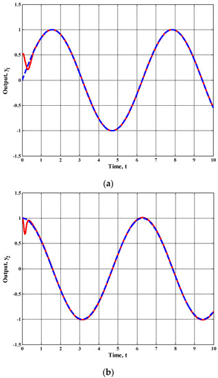
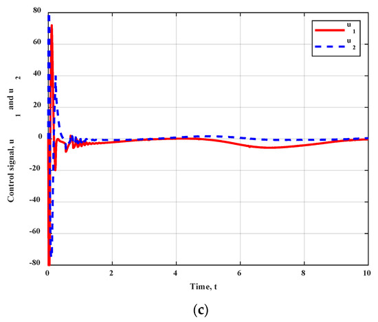
Figure 2. The output response of the hypothetical MIMO system controlled by ADRC based on LESO (a) output curve, $y_1$, (b) output curve, $y_2$, and (c) control signals, $u_1$ and $u_2$.

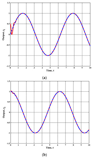
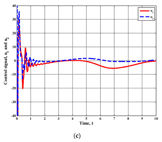
Figure 3. The output response of the hypothetical MIMO system controlled by ADRC based on SMHOESO (a) output curve, $y_1$, (b) output curve, $y_2$, and (c) control signals, $u_1$ and $u_2$.

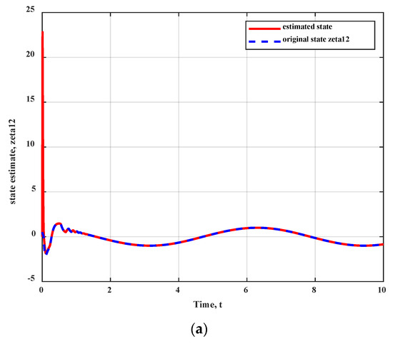
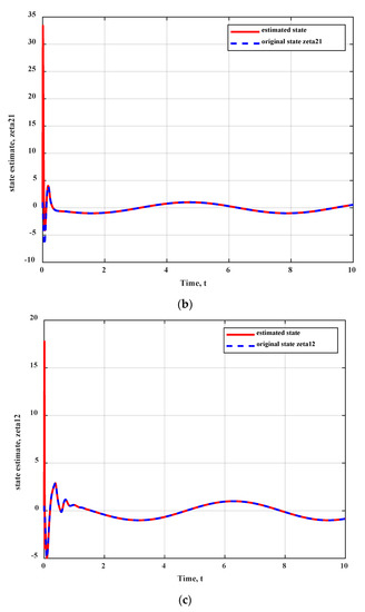
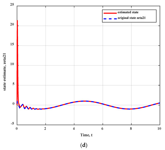
Figure 4. The estimated states response of the hypothetical MIMO system controlled by ADRC based on LESO and SMHOESO (a) state estimate ${\widehat{\xi }}_{\mathrm{1,2}}$ using LESO, (b) state estimate ${\widehat{\xi }}_{\mathrm{2,1}}$ using LESO, (c) state estimate ${\widehat{\xi }}_{\mathrm{1,2}}$ using SMHOESO, and (d) state estimate ${\widehat{\xi }}_{\mathrm{2,1}}$ using SMHOESO.

Table 2. The numerical results of case study 2.

Performance Index	LESO	SMHOESO	%Reduction
ISU1	314.1064	308.4248	1.8%
ISU2	296.8865	225.7019	24%
ITAE1	0.1628	0.1210	25.7%
ITAE2	0.3536	0.0937	73.5%

As shown in Table 2, the proposed configuration resulted in a significant reduction in the ITAE and ISU of the two channels. This is reflected in the control efforts u₁ and u₂ depicted in Figure 2c and Figure 3c, where u₁ and u₂ for the SMHOESO-based ADRC witnessed less activity than the LESO-based ADRC. The SMHOESO-based ADRC has a better tracking output response than the LESO-based ADRC, particularly during the transient period, where both configurations have completely attenuated the effect of the exogenous disturbances w₁ and w₂, the state couplings for each subsystem, and the time-varying input gains b_1,1, b_1,2, b_2,1, and b_2,2 on the output response of the two channels.

Case Study 2: DDMR System

The mathematical model of the mobile robot is an approximation of the physical mobile robot shown in Figure 5; which, is comprised of permanent magnet DC motors (PMDC), wheels dynamic model, DDMR dynamic model, DDMR Kinematic model, and the Tractive forces equation. In this model, it is assumed that the lateral slip and forces arising from dynamic effects are neglected. Lateral slip is zero for straight-line motions and it can be neglected when the vehicle turns “on the spot” or at low velocities [43,44,45,46,47].

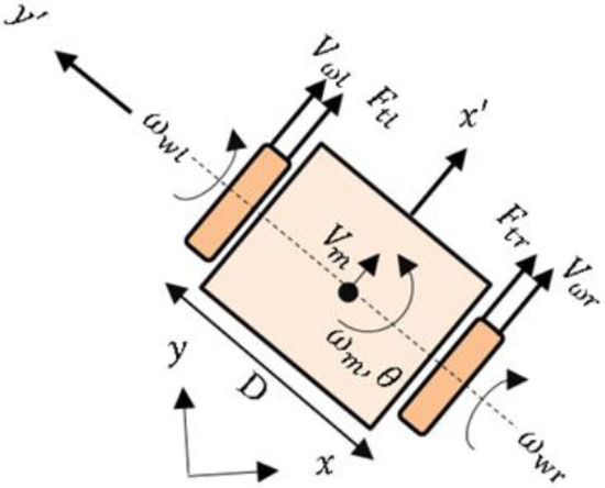
Figure 5. The Differential drive mobile robot.

PMDC motors and the wheels dynamic model is given as [48,49,50],

$$\left\{\begin{array}{c}\begin{array}{c}{\dot{\xi }}_1={\xi }_2\hfill \\ {\dot{\xi }}_2=-\frac{{R_a{B}_{eq}+K}_t{K}_b}{L_a{J}_{eq}}{\xi }_1-\frac{\left(L_a{B}_{eq}+R_a{J}_{eq}\right)}{L_a{J}_{eq}}{\xi }_2+\frac{1}{n}\frac{K_t}{L_a{J}_{eq}}{(v}_{ar}-\frac{L_a}{K_t}{\dot{T}}_{Lr}-\frac{R_a}{K_t}{T}_{Lr})\hfill \\ {\dot{\xi }}_3={\xi }_4\hfill \end{array}\hfill \\ \begin{array}{c}{\dot{\xi }}_4=-\frac{{R_a{B}_{eq}+K}_t{K}_b}{L_a{J}_{eq}}{\xi }_3-\frac{\left(L_a{B}_{eq}+R_a{J}_{eq}\right)}{L_a{J}_{eq}}{\xi }_4+\frac{1}{n}\frac{K_t}{L_a{J}_{eq}}{(v}_{al}-\frac{L_a}{K_t}{\dot{T}}_{Ll}-\frac{R_a}{K_t}{T}_{Ll})\hfill \\ T_{Lr}=\frac{r_w}{n}{F}_{tr}\left({\lambda }_r\right)+\frac{1}{n}{\tau }_{e\xi tr}\hfill \\ T_{Ll}=\frac{r_w}{n}{F}_{tl}\left({\lambda }_l\right)+\frac{1}{n}{\tau }_{e\xi tl}\hfill \end{array}\hfill \end{array}\right.$$

where the state vector ${\left({\xi }_1,{\xi }_2,{\xi }_3,{\xi }_4\right)}^T={\left(\begin{array}{ccc}{\omega }_{wr},& {\dot{\omega }}_{wr},& {\omega }_{wl}\end{array},{\dot{\omega }}_{wl}\right)}^T$ represents the right wheel angular velocity, the right wheel angular acceleration, the left wheel angular velocity, and the left wheel angular acceleration, respectively; $J_{eq}$ is the total equivalent inertia, $k_t$ is the torque constant, $R_a$ is the electric resistance, $B_{eq}$ is the total equivalent damping, $v_{ar}$ and $v_{al}$ are the input voltages applied to the right and left motors, respectively; n is the gearbox ratio, $k_b$ is the voltage constant, $L_a$ is the electric self-inductance constant, and ${\tau }_{e\xi tr},{\tau }_{e\xi tl}$ are the external torque disturbances applied at the right and left wheel sides, respectively. The DDMR dynamic model is given as [51,52,53]:

$$\left\{\begin{array}{c}M{\dot{\xi }}_5=F_{tr}+F_{tl}\hfill \\ J{\dot{\xi }}_6={(F}_{tr}-F_{tl})\frac{D_w}{2}\hfill \end{array}\right.$$

The state vector ${\left({\xi }_5,{\xi }_6\right)}^T={\left(V_m,{\omega }_m\right)}^T$ represents the longitudinal velocity of the center of mass, and the angular velocity of the DDMR. Where $D_w$ is the distance between the right and left wheels of the DDMR, M is the effective mass of the DDMR with the driving wheels and the motors, J is the moment of inertia of the DDMR with the driving wheels and the motors taken at the center of mass about the vertical axis, and $F_{tr}$ and $F_{tl}$ are the tractive forces. The DDMR Kinematic model s given as,

$$\left\{\begin{array}{c}{\dot{\xi }}_7={\xi }_{5}cos\left({\xi }_9\right)\hfill \\ {\dot{\xi }}_8={\xi }_{5}sin\left({\xi }_9\right)\hfill \\ {\dot{\xi }}_9={\xi }_6\hfill \end{array}\right.$$

The state vector ${\left({\xi }_7,{\xi }_8,{\xi }_9\right)}^T={\left(\begin{array}{ccc}{\xi }^{\prime },& y^{\prime },& \theta \end{array}\right)}^T$ represents the Cartesian position in the coordinate system for the DDMR reference frame, and the orientation angle of the DDMR, respectively. The tractive forces equation [51,54,55,56,57],

$$\begin{array}{c}{\xi }_1^s=\frac{1}{r_w}{\xi }_5+\frac{D_w}{2r_w}{\xi }_6\\ {\xi }_3^s=\frac{1}{r_w}{\xi }_5-\frac{D_w}{2r_w}{\xi }_6\\ {\lambda }_r=\frac{{\xi }_1-{\xi }_1^s}{\mathrm{m}\mathrm{a}\mathrm{x}({\xi }_1,{\xi }_1^{\prime })}\\ {\lambda }_l=\frac{{\xi }_3-{\xi }_3^s}{\mathrm{m}\mathrm{a}\mathrm{x}({\xi }_3,{\xi }_3^{\prime })}\\ \mu \left({\lambda }_r\right)=D\mathrm{s}\mathrm{i}\mathrm{n}(C{tan}^{-1}\left(B{\lambda }_r-E\left(B{\lambda }_r-{\tan }^{-1}\left(B{\lambda }_r\right))\right)\right)\\ \mu \left({\lambda }_l\right)=D\mathrm{s}\mathrm{i}\mathrm{n}(C{tan}^{-1}\left(B{\lambda }_l-E\left(B{\lambda }_l-{\tan }^{-1}\left(B{\lambda }_l\right))\right)\right)\\ F_{tr}\left({\lambda }_r\right)=\mu \left({\lambda }_r\right)N\\ F_{tl}\left({\lambda }_l\right)=\mu \left({\lambda }_l\right)N\end{array}$$

where ${\xi }_1^s,{\xi }_3^s$ are relative to the ground linear velocities of the left and right wheels of the WMR in the presence of wheel slipping, respectively, $r_w$ is the nominal radius of the tire, μ represents the adhesive coefficient, which is highly dependent on tire characteristics and the terrain conditions (such as dry, gravel, and ice), and N is the vertical load. The Magic Formula is characterized by four dimensionless coefficients (B, C, D, E), i.e., stiffness, shape, peak, and curvature. The sample data are given in Table 3 and Table 4.

Table 3. Parameters of the ADRC units.

Unit	Parameter	Value
LESO	${\omega }_0$	4.7400
	$b$	14.8378
TD	$R$	19.1324
fal-based control law	${\alpha }_1$	0.5000
	${\delta }_1$	0.0100
	${\alpha }_2$	0.2500
	${\delta }_2$	0.0100
SMHOESO	${\omega }_0$	3.9816
	$a_1$	4
	$a_2$	5.4
	$a_3$	2.88
	$a_4$	0.82
	$\alpha$	0.99
	$\beta$	0.9
	$k_{\alpha }$	2.1
	$k_{\beta }$	0.04

Table 4. The parameters of the robot chassis.

Parameter Name	Parameter Symbol	Value	Unit
Mass	$M$	8.4	kg
The distance between wheels	$D_w$	0.28	m
Wheel radius	$r$	0.075	m
Depth	$a$	0.31	m
Width	$b$	0.29	m
Inertia	$J$	0.1261	kg·m2

Figure 6 shows the applied aperiodic disturbance while Figure 7 shows how the LESO-based ADRC scheme responds to the right and left wheels’ respective angular velocities of ${\omega }_{wr}$ (RPM) and ${\omega }_{wl}$ (RPM). Additionally, Figure 8 clearly depicts how the SMHOESO-based ADRC outperforms the LESO-based ADRC. Figure 8e shows the control signals $u_1$ and $u_2$ generated by the proposed SMHOESO-based ADRC control scheme. It is evidently that the proposed SMHOESO totally removes the chattering in the control signal as compared to the LESO (See Figure 7e). Figure 7 and Figure 8 showed that utilizing the LESO-based ADRC scheme, the rising time of the wheels’ angular velocities, ${\omega }_{wr}$ (RPM) and ${\omega }_{wl}$ (RPM), was longer than when using the SMHOESO-based ADRC scheme as can be seen from the close-up figures (Figure 7b and Figure 8b). Therefore, it is evident that the SMHOESO-based ADRC system yields a quicker response. Additionally, as shown in Figure 8a,c, the final point that can be reached in the actual trajectory of the DDMR for the SMHOESO-based ADRC scheme was closer to the final point of the reference trajectory.

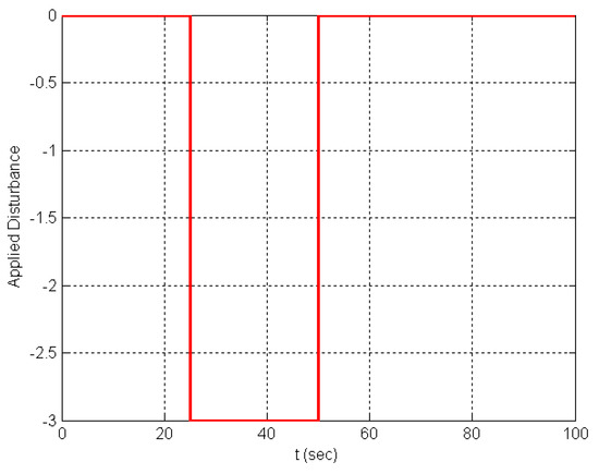
Figure 6. The applied external torque.

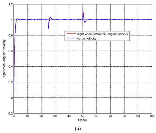
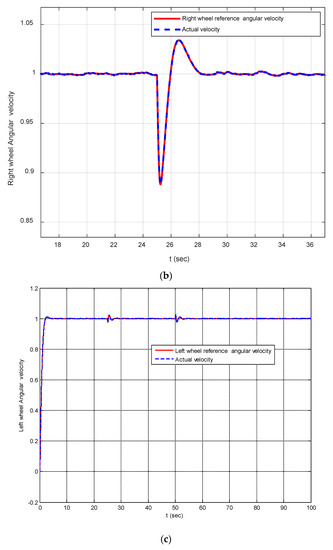
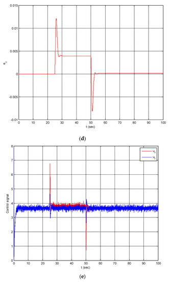
Figure 7. Output results for LESO, (a) The right wheel angular velocity, (b) close-up of (a), (c) The left wheel angular velocity, (d) the orientation error of the DDMR, and (e) the control signal.

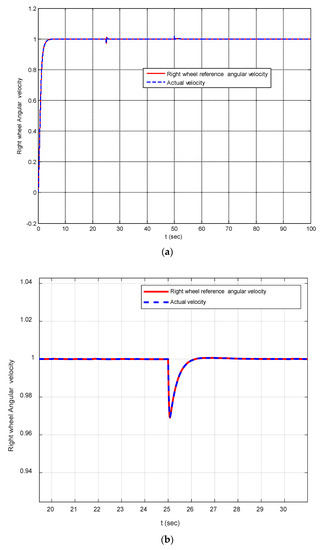
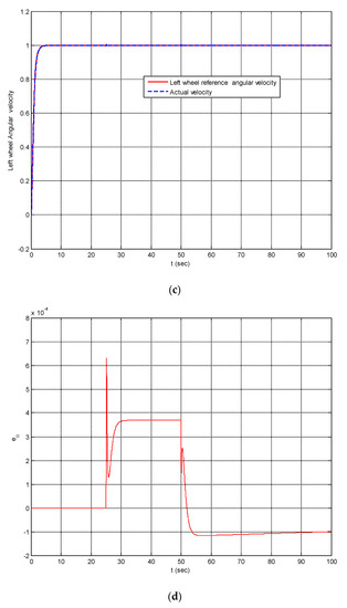
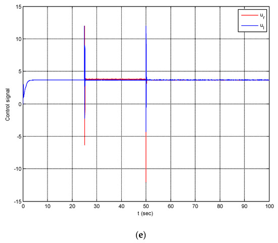
Figure 8. Output results for SMHOESO, (a) the right wheel angular velocity, (b) close-up of (a), (c) the left wheel angular velocity, (d) the orientation error of the DDMR, and (e) the control signal.

The kinematic index (see Table 5) for the ADRC based on SMHOESO significantly improved as compared to the traditional ADRC, with an ${OPI}_{\theta }$ reduction of 99.3447%. The simulations (see Table 6) demonstrate that, in contrast to a discernible improvement in the transient response, the ISU, which indicates the energy given to the PMDC motor, has unintentionally increased. In addition, the suggested observer almost eliminates the chattering in the control signal brought on by Han’s traditional ADRC.

Table 5. The DDMR kinematics index.

Performance Index	Observer Type
	LESO	SMHOESO
OPIθ	0.0000057838	0.0000000379

Table 6. Performance measures of both wheels.

Wheel	Performance Measure	Observer Type
		LESO	SMHOESO
Right	ITAE	10.537531	1.045611
	ISU	1349.853127	1376.019003
Left	ITAE	5.126353	0.720233
	ISU	1323.280874	1333.229224

As a final comparison between the proposed SMHOESO and the conventional LESO, a step change in the torque disturbance of 3 N.M applied at 25 s; the result (Figure 9) shows that the proposed SMHOESO outperforms the conventional LESO where the undershoot and the overshoot are apparently removed. While the LESO exhibits chattering, the proposed SMHOESO totally removes the chattering from the output response and settles at faster settling time of 26 s, while the output response in the LESO settles at 34 s.

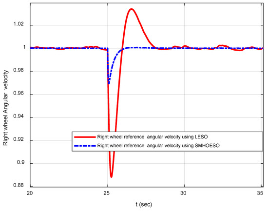
Figure 9. Comparison between the proposed SMHOESO and the conventional LESO.

where ITAE is the Integral Time-weighted Absolute Error (ITAE) and is defined as ITAE = ${\int }_0^{t_f}t\left|e\right|dt$, ISU is the Integration of the square of the controller energy and is defined as ISU = ${\int }_0^{t_f}{u}^2(t)dt$, and finally ${OPI}_{\theta }=\frac{1}{N}{\sum \left({\theta }_{ref}-{\theta }_{actual}\right)}^2$.

6. Conclusions

This paper demonstrated a methodology based on an innovative high-gain observer class of ESO. If the initial estimation error is large, such high gains may result in the peak phenomenon, rendering the linear ESO impractical or even dangerous to use. This work includes two significant enhancements. First, a nonlinear error function with smoothness, a high gain near the origin, and a small gain for large error values is used. Second, these improvements are required due to the higher-order extended observer; which, allows for an accurate estimation of high-order total disturbance. These enhancements resulted in both a smooth control signal provided by the suggested observer and a minimum overshoot in the output response. It can be concluded that the proposed observers successfully achieved the desired response for the DDMR and produced less chattering control signals and better time-domain performance in terms of steady-state error and transient responses. The current work will be followed by a fractional order control to design the three parts of the ADRC to produce a fractional-order ADRC. Furthermore, a practical implementation of this technique on a well-known application will highlight the method’s distinguishing feature. Another piece of future work is to conduct the H/W implementation of the proposed SMHOESO on the DDMR platform, and testing and validating the obtained results.

References

- Pu, Z.; Yuan, R.; Yi, J.; Tan, X. A Class of Adaptive Extended State Observers for Nonlinear Disturbed Systems. IEEE Trans. Ind. Electron. 2015, 62, 5858–5869. [Google Scholar] [CrossRef]
- Gaol, L.Q. On stability analysis of active disturbance rejection control for nonlinear time-varying plants with unknown dynamics. In Proceedings of the 2007 46th IEEE Conference on Decision and Control, New Orleans, LA, USA, 12–14 December 2007; pp. 3501–3506. [Google Scholar]
- Pu, Z.; Yuan, R.; Yi, J.; Tan, X. Design and Analysis of Time-varying Extended State Observer. In Proceedings of the 2015 34th Chinese Control Conference (CCC), Hangzhou, China, 28–30 July 2015; pp. 753–758. [Google Scholar]
- Yoo, D.; Yau, T.; Gao, Z.; Yooy, D.; Gaoz, Z. Optimal fast tracking observer bandwidth of the linear extended state observer. Int. J. Control 2007, 80, 102–111. [Google Scholar] [CrossRef]
- Krishna Srinivasan, M.; Daya John Lionel, F.; Subramaniam, U.; Blaabjerg, F.; Madurai Elavarasan, R.; Shafiullah, G.M.; Khan, I.; Padmanaban, S. Real-Time Processor-in-Loop Investigation of a Modified Non-Linear State Observer Using Sliding Modes for Speed Sensorless Induction Motor Drive in Electric Vehicles. Energies 2020, 13, 4212. [Google Scholar] [CrossRef]
- Sakthivel, N.; Mounika Devi, M.; Alzabut, J. H∞ observer-based consensus for nonlinear multiagent systems with actuator saturation and input delays. Int. J. Control 2022. [Google Scholar] [CrossRef]
- Jayaramu, M.L.; Suresh, H.N.; Bhaskar, M.S.; Almakhles, D.; Padmanaban, S.; Subramaniam, U. Real-Time Implementation of Extended Kalman Filter Observer With Improved Speed Estimation for Sensorless Control. IEEE Access 2021, 9, 50452–50465. [Google Scholar] [CrossRef]
- Guo, B.Z.; Zhao, Z.L. On the convergence of an extended state observer for nonlinear systems with uncertainty. Syst. Control Lett. 2011, 60, 420–430. [Google Scholar] [CrossRef]
- Zhao, Z.-L.; Guo, B.-Z. On convergence of non-linear extended state observer for multi-input multi-output systems with uncertainty. IET Control Theory Appl. 2012, 6, 2375–2386. [Google Scholar]
- KINETIS MOTOR SUITE: Sensorless PMSM Field-Oriented Control on Kinetis KV and KE. Available online: https://www.nxp.com/doc/AN5237 (accessed on 1 May 2022).
- Ibraheem, I.K.; Abdul-Adheem, W.R. An Improved Active Disturbance Rejection Control for a Differential Drive Mobile Robot with Mismatched Disturbances and Uncertainties. In Proceedings of the Third International Conference on Electrical and Electronic Engineering, Telecommunication Engineering and Mechatronics (EEETEM2017), Beirut, Lebanon, 26–28 April 2017; pp. 7–12. [Google Scholar]
- Achieve Improved Motion and Efficiency for Advanced Motor Control Designs In Minutes with TI’s New InstaSPINTM-MOTION Technology. Texas Instruments. Available online: http://www.prnewswire.com/news-releases/achieve-improved-motion-and-efficiency-for-advanced-motor-control-designs-in-minutes-with-tis-new-instaspin-motion-technology-203572121.html (accessed on 1 May 2022).
- Huang, Y.; Xue, W.; Zhiqiang, G.; Sira-Ramirez, H.; Wu, D.; Sun, M. Active disturbance rejection control: Methodology, practice and analysis. In Proceedings of the 33rd Chinese Control Conference, Nanjing, China, 28–30 July 2014; pp. 1–5. [Google Scholar] [CrossRef]
- Wang, W.; Gao, Z. A comparison study of advanced state observer design techniques. In Proceedings of the 2003 American Control Conference, 2003, Denver, CO, USA, 4–6 June 2003; Volume 6, pp. 4754–4759. [Google Scholar] [CrossRef]
- Gao, Z. Scaling and bandwidth-parameterization based controller tuning. In Proceedings of the American Control Conference 2003, Denver, CO, USA, 4–6 June 2003; Volume 6, pp. 4989–4996. [Google Scholar]
- Sun, L.; Li, D.; Hu, K.; Lee, K.Y.; Pan, F. On Tuning and Practical Implementation of Active Disturbance Rejection Controller: A Case Study from a Regenerative Heater in a 1000 MW Power Plant. Ind. Eng. Chem. Res. 2016, 55, 6686–6695. [Google Scholar] [CrossRef]
- Bao, D.; Tang, W. Adaptive sliding mode control of ball screw drive system with extended state observer. In Proceedings of the 2016 2nd International Conference on Control, Automation and Robotics (ICCAR), Hong Kong, China, 28–30 April 2016; pp. 133–138. [Google Scholar]
- Godbole, A.A.; Kolhe, J.P.; Talole, S.E. Performance analysis of generalized extended state observer in tackling sinusoidal disturbances. IEEE Trans. Control Syst. Technol. 2013, 21, 2212–2223. [Google Scholar] [CrossRef]
- Pan, H.; Sun, W.; Gao, H.; Hayat, T.; Alsaadi, F. Nonlinear tracking control based on extended state observer for vehicle active suspensions with performance constraints. Mechatronics 2015, 30, 363–370. [Google Scholar] [CrossRef]
- Yang, L.; Liu, L.; Zhang, J. A bi-bandwidth extended state observer for a system with measurement noise and its application to aircraft with abrupt structural damage. Aerosp. Sci. Technol. 2021, 114, 106742. [Google Scholar] [CrossRef]
- Li, Y.; Yang, B.; Zheng, T.; Li, Y.; Cui, M.; Peeta, S. Extended-State-Observer-Based Double-Loop Integral Sliding-Mode Control of Electronic Throttle Valve. IEEE Trans. Intell. Transp. Syst. 2015, 16, 2501–2510. [Google Scholar] [CrossRef]
- Goel, A.; Swarup, A. Performance Analysis of Active Disturbance Rejection Controlled Robotic Manipulator based on Evolutionary Algorithm. Int. J. Hybrid Inf. Technol. 2016, 9, 65–80. [Google Scholar] [CrossRef]
- Ma, Q.; Xu, D.; Lv, P.; Shi, Y. Application of NSGA-II in Parameter Optimization of Extended State Observer. In Challenges of Power Engineering and Environment; Cen, K., Chi, Y., Wang, F., Eds.; Springer: Berlin/Heidelberg, Germany, 2007; pp. 587–592. [Google Scholar] [CrossRef]
- Zheng, M.; Chen, X.; Tomizuka, M. Extended state observer with phase compensation to estimate and suppress high-frequency disturbances. In Proceedings of the 2016 American Control Conference (ACC), Boston, MA, USA, 6–8 July 2016; pp. 3521–3526. [Google Scholar] [CrossRef]
- Lee, S.; Kim, Y. Design of nonlinear observer for strap-down missile guidance law via sliding mode differentiator and extended state observer. In Proceedings of the 2016 International Conference on Advanced Mechatronic Systems (ICAMechS), Melbourne, Australia, 30 November–3 December 2016; pp. 143–147. [Google Scholar]
- Liu, B.; Jin, Y.; Chen, C.; Yang, H. Speed Control Based on ESO for the Pitching Axis of Satellite Cameras. Math. Probl. Eng. 2016, 2016, 2138190. [Google Scholar] [CrossRef]
- Li, J.; Qi, X.; Xia, Y.; Pu, F.; Chang, K. Frequency domain stability analysis of nonlinear active disturbance rejection control system. ISA Trans. 2014, 56, 188–195. [Google Scholar] [CrossRef]
- Mao, J.; Gu, L.; Wu, A.; Wu, G.; Zhang, X.; Chen, D. Back-stepping control for vertical axis wind power generation system maximum power point tracking based on extended state observer. In Proceedings of the 2016 35th Chinese Control Conference (CCC), Chengdu, China, 27–29 July 2016; pp. 8649–8653. [Google Scholar] [CrossRef]
- Yang, H.; Yu, Y.; Yuan, Y.; Fan, X. Back-stepping control of two-link flexible manipulator based on an extended state observer. Adv. Sp. Res. 2015, 56, 2312–2322. [Google Scholar] [CrossRef]
- Xia, Y.; Yang, H.; You, X.; Li, H. Adaptive control for attitude synchronisation of spacecraft formation via extended state observer. IET Control Theory Appl. 2014, 8, 2171–2185. [Google Scholar]
- Lin, Y.P.; Lin, C.L.; Suebsaiprom, P.; Hsieh, S.L. Estimating evasive acceleration for ballistic targets using an extended state observer. IEEE Trans. Aerosp. Electron. Syst. 2016, 52, 337–349. [Google Scholar] [CrossRef]
- Wu, S.; Dong, B.; Ding, G.; Wang, G.; Liu, G.; Li, Y. Backstepping sliding mode force/position control for constrained reconfigurable manipulator based on extended state observer. In Proceedings of the 2016 12th World Congress on Intelligent Control and Automation (WCICA), Guilin, China, 12–15 June 2016; pp. 477–482. [Google Scholar] [CrossRef]
- Duan, H.; Tian, Y.; Wang, G. Trajectory tracking control of ball and plate system based on auto-disturbance rejection controller. In Proceedings of the 2009 7th Asian Control Conference, Hong Kong, China, 27–29 August 2009; pp. 471–476. [Google Scholar]
- Benxian, X.; Ping, W.; Xueping, D.; Xingpeng, Z.; Haibin, Y. Study on nonlinear friction compensation for bi-axis servo system based-on ADRC. In Proceedings of the International Conference on Information Science and Technology, Nanjing, China, 26–28 March 2011; pp. 788–793. [Google Scholar] [CrossRef]
- Liu, D.; Che, C.; Zhou, Z. Permanent magnet synchronous motor control system based on auto disturbances rejection controller. In Proceedings of the 2011 International Conference on Mechatronic Science, Electric Engineering and Computer (MEC), Jilin, China, 19–22 August 2011; pp. 8–11. [Google Scholar] [CrossRef]
- Abdul-adheem, W.R.; Ibraheem, I.K. From PID to Nonlinear State Error Feedback Controller. IJACSA 2017, 8, 312–322. [Google Scholar]
- Kang, Y.L.; Shrestha, G.B.; Lie, T.T. Application of an NLPID controller on a UPFC to improve transient stability of a power system. IEE Proc.—Gener. Transm. Distrib. 2001, 148, 523–529. [Google Scholar] [CrossRef]
- Ma, L.; Lin, F.; You, X.; Zheng, T.Q. Nonlinear PID control of three-phase pulse width modulation rectifier. In Proceedings of the 2008 7th World Congress on Intelligent Control and Automation, Chongqing, China, 25–27 June 2008; pp. 3417–3422. [Google Scholar] [CrossRef]
- Ajeil, F.; Ibraheem, I.K.; Azar, A.T.; Humaidi, A.J. Autonomous Navigation and Obstacle Avoidance of an Omnidirectional Mobile Robot Using Swarm Optimization and Sensors Deployment. Int. J. Adv. Robot. Syst. 2020, 17, 1–15. [Google Scholar] [CrossRef]
- Najm, A.A.; Ibraheem, I.K.; Azar, A.T.; Humaidi, A.J. Genetic Optimization-Based Consensus Control of Multi-Agent 6-DoF UAV System. Sensors 2020, 20, 3576. [Google Scholar] [CrossRef] [PubMed]
- Lenain, R.; Thuilot, B.; Cariou, C.; Martinet, P. Adaptive and Predictive Path Tracking Control for Off-road Mobile Robots. Eur. J. Control 2007, 13, 419–439. [Google Scholar] [CrossRef]
- Le, A.T. Modelling and Control of Tracked Vehicles; The University of Sydney: Camperdown, Australia, 1999. [Google Scholar]
- Kitano, M.; Kuma, M. An analysis of horizontal plane motion of tracked vehicles. J. Terramechanics 1977, 14, 211–225. [Google Scholar] [CrossRef]
- Ibraheem, G.A.R.; Azar, A.T.; Ibraheem, I.K.; Humaidi, A.J. A Novel Design of a Neural Network-based Fractional PID Controller for Mobile Robots Using Hybridized Fruit Fly and Particle Swarm Optimization. Complexity 2020, 2020, 3067024. [Google Scholar] [CrossRef]
- Ajeil, F.H.; Ibraheem, I.K.; Azar, A.T.; Humaidi, A.J. Grid-Based Mobile Robot Path Planning Using Aging-Based Ant Colony Optimization Algorithm in Static and Dynamic Environments. Sensors 2020, 20, 1880. [Google Scholar] [CrossRef] [PubMed]
- Abdul-adheem, W.R.; Ibraheem, I.K. Improved Sliding Mode Nonlinear Extended State Observer based Active Disturbance Rejection Control for Uncertain Systems with Unknown Total Disturbance. Int. J. Adv. Comput. Sci. Appl. 2016, 7, 80–93. [Google Scholar]
- Partovibakhsh, M. Adaptive Unscented Kalman Filter-Based Online Slip Ratio Control of Wheeled-Mobile Robot. In Proceedings of the 11th World Congress on Intelligent Control and Automation, Shenyang, China, 29 June–4 July 2014; pp. 6161–6166. [Google Scholar]
- Subudhi, B.; Ge, S. Sliding-mode-observer-based adaptive slip ratio control for electric and hybrid vehicles. IEEE Trans. Intell. Transp. Syst. 2012, 13, 1617–1626. [Google Scholar] [CrossRef]
- Tian, Y.; Sarkar, N. Control of a mobile robot subject to wheel slip. J. Intell. Robot. Syst. Theory Appl. 2014, 74, 915–929. [Google Scholar] [CrossRef]
- Balakrishna, R.; Ghosal, A. Modeling of Slip For Wheeled Mobile Robots. IEEE Trans. Robot. Autom. 1995, 11, 126–132. [Google Scholar] [CrossRef]
- Liaw, D.-C.; Chung, W.-C. Control Design for Vehicle’s Lateral Dynamics. In Proceedings of the 2006 IEEE International Conference on Systems, Man and Cybernetics, Taipei, Taiwan, 8–11 October 2006; pp. 2081–2086. [Google Scholar] [CrossRef]
- Ming, Q. Sliding Mode Controller Design for ABS System. Master’s Thesis, Faculty of the Virginia Polytechnic Institute and State University, Blacksburg, VA, USA, 1997. Available online: http://hdl.handle.net/10919/30598 (accessed on 1 May 2022).
- Li, J.; Song, Z.; Shuai, Z.; Xu, L.; Ouyang, M. Wheel Slip Control Using Sliding-Mode Technique and Maximum Transmissible Torque Estimation. J. Dyn. Syst. Meas. Control 2015, 137, 111010. [Google Scholar] [CrossRef]
- Ahmed, S.; Azar, A.T.; Tounsi, M. Adaptive Fault Tolerant Non-Singular Sliding Mode Control for Robotic Manipulators Based on Fixed-Time Control Law. Actuators. 2022, 11, 353. [Google Scholar] [CrossRef]
- Sidek, S.N. Dynamic Modeling and Control of Nonholonomic Wheeled Mobile Robot Subjected to Wheel Slip; The Faculty of the Graduate School of Vanderbilt University: Nashville, TN, USA, 2008. [Google Scholar]
- Ma, Y.-K.; Raja, M.M.; Nisar, K.S.; Shukla, A.; Vijayakumar, V. Results on controllability for Sobolev type fractional differential equations of order 1 < r < 2 with finite delay. AIMS Math. 2022, 7, 10215–10233. [Google Scholar] [CrossRef]
- Raja, M.M.; Vijayakumar, V.; Shukla, A.; Nisar, K.S.; Baskonus, H.M. On the approximate controllability results for fractional integrodifferential systems of order 1 < r < 2 with sectorial operators. J. Comput. Appl. Math. 2022, 415, 114492. [Google Scholar] [CrossRef]
Disclaimer/Publisher’s Note: The statements, opinions and data contained in all publications are solely those of the individual author(s) and contributor(s) and not of MDPI and/or the editor(s). MDPI and/or the editor(s) disclaim responsibility for any injury to people or property resulting from any ideas, methods, instructions or products referred to in the content. |
© 2023 by the authors. Licensee MDPI, Basel, Switzerland. This article is an open access article distributed under the terms and conditions of the Creative Commons Attribution (CC BY) license (https://creativecommons.org/licenses/by/4.0/).