Design and Microscale Fabrication of Negative Poisson’s Ratio Lattice Structure Based on Multi-Scale Topology Optimization

Abstract

The current design of negative Poisson’s ratio lattice structures is mainly forward-looking and predominantly dependent on several known deformation patterns. To automate the generation of structures with programmable Poisson’s ratio, the study utilized the energy homogenization method and the Solid Isotropic Material with Penalization (SIMP) method to establish an optimization model for negative Poisson’s ratio. By proposing a relaxed objective function and eliminating damping in the Optimality Criteria (OC) method, the study achieves the automatic evolution of negative Poisson’s ratio programmable lattice unit cells, with the lowest Poisson’s ratio achieving −0.5367, and an equivalent elastic matrix is derived. The iterative process’s efficiency is comparable to that of commercial software, with a maximum iteration time of 300 s, enabling the prompt identification of fundamental configurations. To validate the method’s effectiveness, finite element analysis was performed on four tubular structures, revealing evident tension–compression deformation patterns. Moreover, the microscale selective laser melting was used to successfully prepare multiple sets of tubular samples made from 316L stainless steel, each with a height of 5 mm. Quasi-static compression experiments showed negative Poisson’s ratio effects and buckling forms that align with finite element analysis results, providing valuable insights for industry applications.

1. Introduction

Materials with negative Poisson’s ratio, also known as auxetic materials [1], display unique characteristics where they expand in the direction perpendicular to the applied tensile load, setting them apart from traditional materials. These materials exhibit significantly enhanced compressive strength in the plane, improved fracture toughness, increased transverse shear modulus, and improved dynamic properties, such as energy absorption and wave attenuation [2], when compared to materials with positive Poisson’s ratio. Consequently, negative Poisson’s ratio materials have found widespread applications in various fields, such as self-expanding coronary stents, esophageal stents, medical bandages, helmets, etc., making them one of the most important branches of mechanical metamaterials.

The concept of Poisson’s ratio was initially proposed by the French mathematician Poisson to describe the longitudinal deformation that occurs concurrently with lateral deformation in a material, and most traditional materials exhibit a positive Poisson’s ratio. In the early stages of elasticity theory, the uniconstant theory stated that the Poisson’s ratio of all isotropic materials was 0.25. However, with the development of classical elasticity theory, it became evident that the elastic deformation of isotropic materials can be described by two independent parameters, elastic modulus and Poisson’s ratio, and the Poisson’s ratio values of different materials differ significantly. Currently, classical elasticity theory demonstrates that the Poisson’s ratio of isotropic materials falls within the range of −1.0 to 0.5 [3].

Since the synthesis of the first artificial negative Poisson’s ratio foam by LAKES [4], numerous artificial negative Poisson’s ratio materials/structures have emerged with the advancement of micro-nano processing and 3D additive manufacturing technologies. Based on different deformation mechanisms, these structures can be classified into various types, such as missing rib, rigid/semi-rigid rotation, re-entrant, chiral, and elastic instability. To achieve larger ranges of negative Poisson’s ratio and adjustable elastic anisotropy, Mizzi et al. [5,6] proposed a hexachiral design with less symmetry. They found that the design enhanced functionality and applicability. Additionally, the impact of translational disorder on the Poisson’s ratio of the hexachiral lattice was also investigated. Pozniak et al. [7] utilized finite element methods to determine the Poisson’s ratio of an anti-chiral structure built on a rectangular lattice with randomly distributed circular node sizes. The studied model was parameterized by lattice anisotropy, rib thickness, and the radius distribution of circular nodes. Three methods were developed, and the results showed that, with sufficient anisotropy of the structure, the Poisson’s ratio could reach any negative value, even lower than −1. Thin ribs (t < 0.1) and thin-walled circular nodes had lower Poisson’s ratio values, and a large aspect ratio can be thought of as an efficient amplifier of the strain in the x direction onto the strain in the transverse y direction. Comparing the results obtained by the three different methods, it was found that the approximation based on Timoshenko beams was only effective in the limit of thin ribs, and the difference between them increased with the augment of thickness.

Several novel types of negative Poisson’s ratio metamaterials were also proposed. Idczak et al. [8] employed the moving asymptotes algorithm and a penalty method to design a chiral structure consisting of two opposite quadruple helices. The resulting structure demonstrated a tunable Poisson’s ratio and optimized mechanical properties for isotropic solids. Zhang et al. [9] presented a multi-material chiral lattice structure with negative Poisson’s ratio and stiffness. To achieve this, they utilized a combination of the independent point-wise density interpolation model and bi-material interpolation method. Reference [10] constructed a flexible negative Poisson’s ratio lattice structure composed of interlocked Archimedean spirals. They controlled the adjustable stiffness by manipulating the local intensity of image patterns. Furthermore, references [11,12] designed negative Poisson’s ratio isotropic cubic lattice structures composed of rigid nodules and deformable beams. To study the elastic properties and size effects of these structures, they established a constitutive equation based on isotropic linear Cosserat elasticity. Duan et al. [13] proposed a novel 3D cubic symmetric lattice material with a negative Poisson’s ratio. They derived its elastic constants based on the micropolar continuum theory and homogenization method.

Although the design of negative Poisson’s ratio materials has advanced considerably, the overall design of such structures is still predominantly forward-looking, with significant untapped potential for further innovation. Specifically, the automatic generation of programmable Poisson’s ratio structures using topology optimization needs to be explored, instead of relying on known configurations or mathematical models. Clausen et al. [14] and Wang [15] utilized a hyperelastic material model, incorporating geometric nonlinearity to achieve programmable Poisson’s ratio microstructures under moderate deformation. Zhang et al. [9] used optimization methods to achieve controllable negative Poisson’s ratio properties in multiphase materials, based on practical engineering requirements. With the rapid development of additive manufacturing technology, the preparation of materials with infinite arbitrary topological layouts and complex microstructures has been greatly facilitated. Combining additive manufacturing processes with the controllable design of mechanical metamaterials will be of great significance for the preparation of high-performance structures [16,17,18,19,20,21,22,23]. Therefore, the study established a topology optimization model which can automatically generate point lattice unit cells with programmable negative Poisson’s ratio, filling this kind of gap. By conducting computation, several unit cells with negative Poisson’s ratio were obtained, and the lowest Poisson’s ratio achieved was −0.5367. To validate the effectiveness of the method, finite element analysis was carried out on four tubular structures, revealing clear tension–compression deformation patterns. In addition, 5 mm tubular samples were fabricated using microscale selective laser melting and 316L stainless steel. Quasi-static compression experiments showed that the observed negative Poisson’s ratio effects and buckling forms were consistent with the results obtained from the finite element analysis.

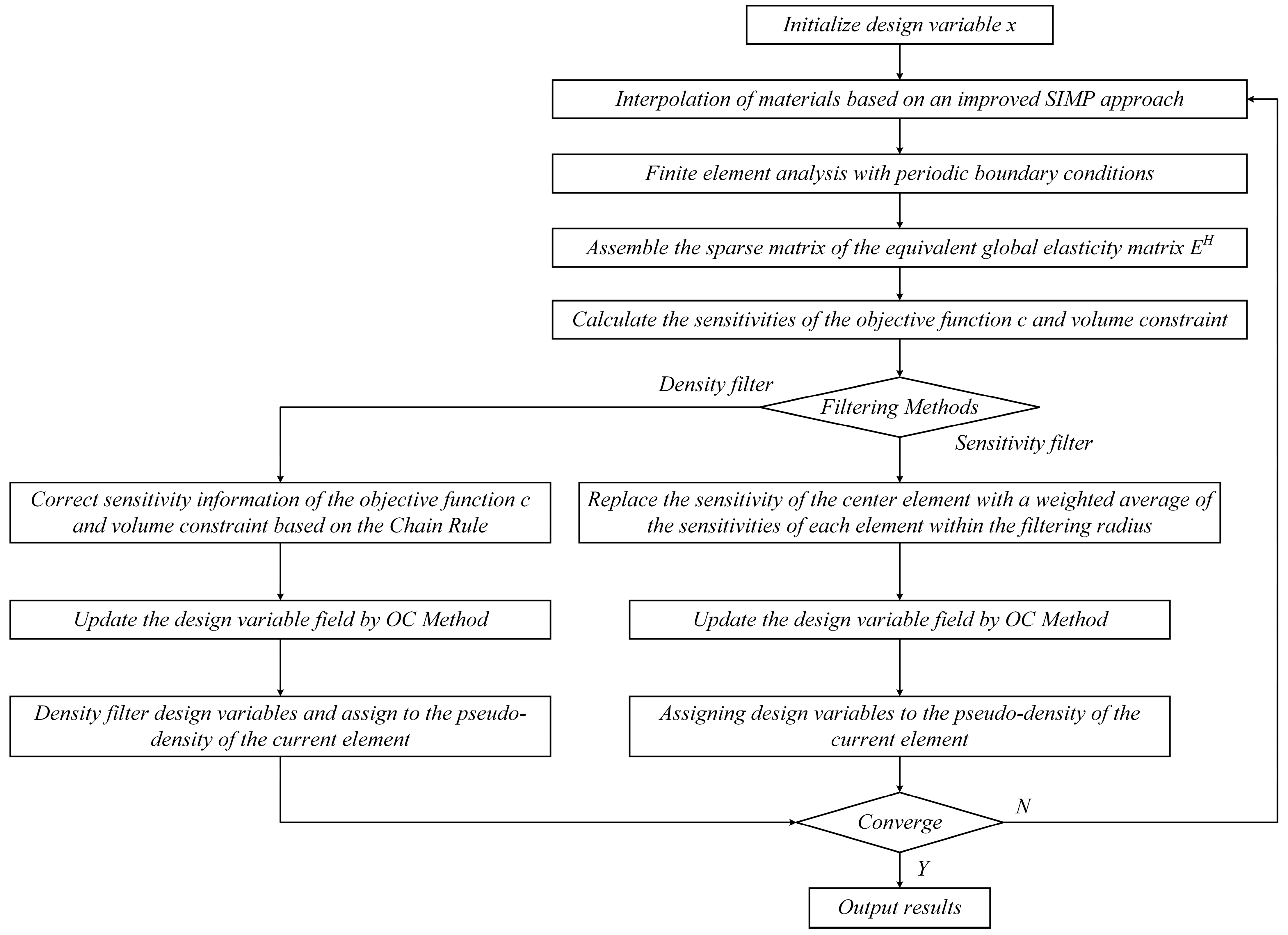
2. Numerical Process

The study focuses on the design of a structure with negative Poisson’s ratio and the maximization of its corresponding effect through optimized tools. To achieve this, we utilized the classic 88-line topology optimization algorithm [24], while the material interpolation model was an improved version of the Solid Isotropic Material with Penalization (SIMP) method [25], a well-established density-based approach. The Optimality Criteria (OC) method [26] was the chosen optimization strategy, and the algorithm incorporated two filtering methods, namely density and sensitivity filters [24]. MATLAB R2018b was utilized as the software platform throughout the entire development process.

The numerical process of simulating structures exhibiting negative Poisson’s ratio is depicted in Figure 1. The global design variable, denoted as the pseudo-density field, was initialized, and material interpolation was performed based on an improved SIMP model. Finite element analysis was then conducted after establishing periodic boundary conditions, and the overall effective elastic stiffness matrix of the current structure was obtained using the energy homogenization method. The objective function, denoted as c, and the sensitivity of the volume constraint were subsequently calculated.

In the case of density filtering, the objective function and sensitivity of the volume constraint would be corrected using the chain rule, and the optimal design would be obtained through the OC method. The design variable field would then be updated, and density filtering would be performed before assigning a pseudo-density to each element. If the sensitivity filter was selected, the sensitivity of each element within the filtering radius would be replaced by the weighted average of the sensitivity values, and the OC method would be used to update the design variable field. The new design variable field would become the current pseudo-density field, and the process would be checked for convergence. If convergence was achieved, the output would be generated, and the design would be plotted. Otherwise, the above steps would be repeated.

The process enhances the compactness of the algorithm based on the 88-line method and aims to extract the finite element analysis process from the loop. The use of the energy homogenization method to obtain the equivalent constitutive parameters greatly simplifies the process. Furthermore, the approach enables the generation of structures exhibiting negative Poisson’s ratio, which has significant practical applications.

3. Energy Homogenization

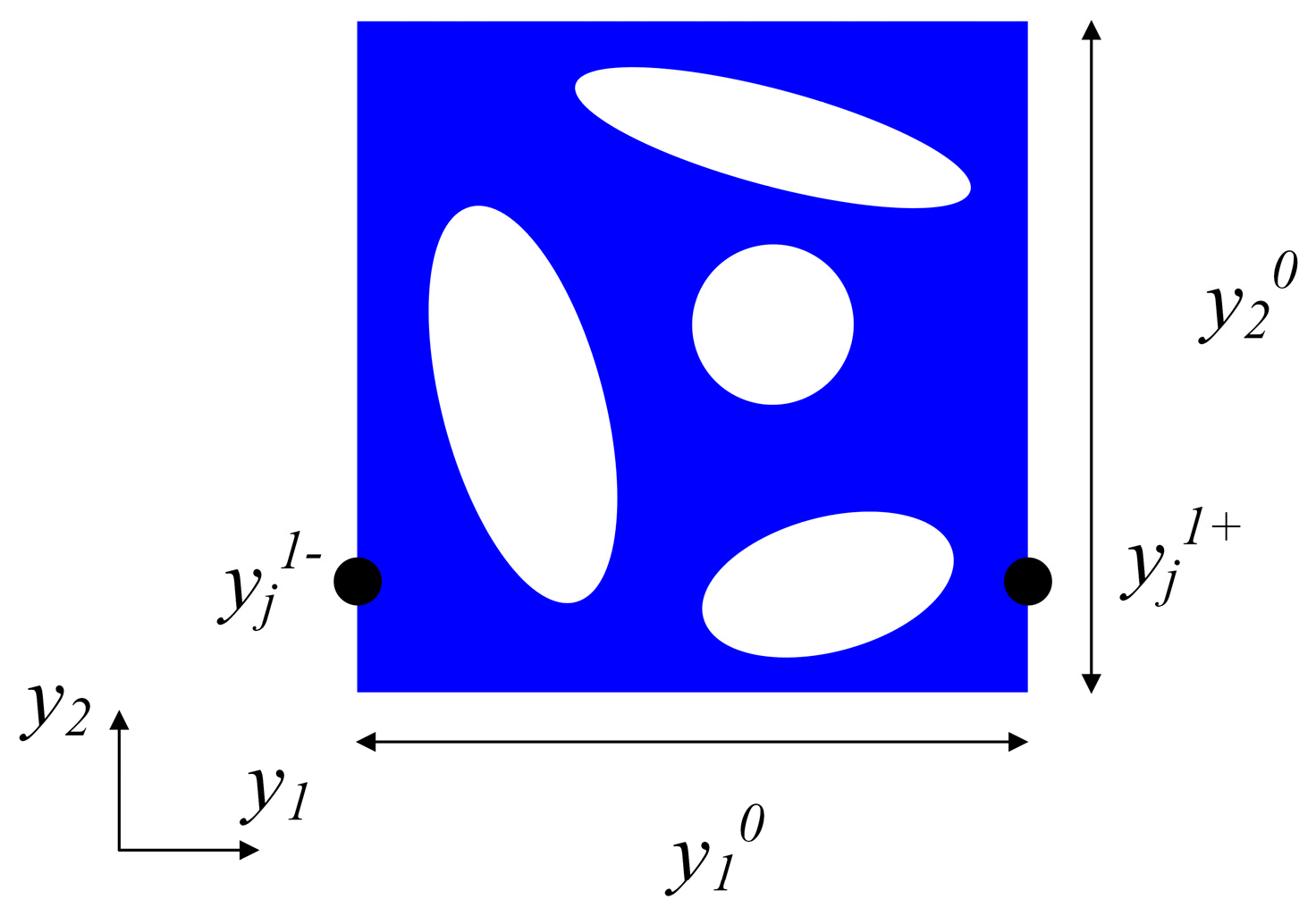
3.1. Periodic Boundary Conditions (PBC)

The equation for energy homogenization under periodic boundary conditions is typically expressed as follows:

$${\int }_Y^{}{E}_{ijpq}{\epsilon }_{pq}^{\ast \left(kl\right)}\frac{\partial v_i}{\partial y_j}dY={\int }_Y^{}{E}_{ijpq}{\epsilon }_{pq}^{0\left(kl\right)}\frac{\partial v_i}{\partial y_j}dY.$$

(1)

By solving the single-cell equilibrium problem under the unit strain ${\epsilon }_{pq}^{0\left(kl\right)}$, the strain field ${\epsilon }_{pq}^{A\left(kl\right)}$ in Equation (1) can be obtained. Under the assumption of periodicity, the displacement field of the cell under the given strain ${\epsilon }_{pq}^{0\left(kl\right)}$ can be written as the sum of the macroscopic displacement field and the periodic fluctuation field $u_i^{*}$:

$$u_i={\epsilon }_{ij}^0{y}_j+u_i^{*}$$

(2)

In fact, Equation (2) cannot be directly applied to the boundary because the periodic fluctuation term $u_i^{*}$ is unknown. Therefore, the above expression needs to be transformed into an explicit constraint between two nodes on the relative surface of the single cell. For a two-dimensional single cell, as shown in Figure 2, a pair of relative boundary displacements can be formulated as

$$\left\{\begin{array}{c}{u}_i^{k+}={\epsilon }_{ij}^0{y}_j^{k+}+u_i^{*}\\ u_i^{k-}={\epsilon }_{ij}^0{y}_j^{k-}+u_i^{*}\end{array}\right.$$

(3)

where the superscripts “k+” and “k−” denote two opposite parallel boundary surfaces perpendicular to the k^th direction (k = 1, 2, 3). Thus, the periodic term $u_i^{*}$ can be obtained from the difference in displacements between the two nodes:

$$u_i^{k+}-u_i^{k-}={\epsilon }_{ij}^0\left(y_j^{k+}-y_j^{k-}\right)={\epsilon }_{ij}^0{\Delta y}_j^k.$$

(4)

For any given parallelepiped cell, ${\Delta y}_j^k$ is constant. For the single cell shown in Figure 2, it can be easily obtained that

$$\begin{gathered} \Delta y_1^1=y_1^1,\Delta y_2^1=0 \\ \Delta y_2^2=y_2^0,\Delta y_1^2=0, \end{gathered}$$

(5)

and when ${\epsilon }_{ij}^0$ is given, the right-hand side of the equation becomes a constant, denoted as $w_j^k$:

$$\begin{gathered} u_i^{k+}-u_i^{k-}=w_i^k \\ {w}_i^k={\epsilon }_{ij}^0{\Delta y}_j^k. \end{gathered}$$

(6)

This particular form of boundary condition is readily applicable to the finite element model through the imposition of constraints upon the corresponding node displacements. Additionally, it simultaneously fulfills the imperatives of periodicity and continuity in the context of displacement based finite element analysis.

3.2. The Numerical Solution of the Equation for Energy Homogenization

In instances where both the geometry and loading exhibit symmetry, the use of periodic boundary conditions can be substituted with regular boundary conditions, as exemplified in the case studies discussed in this paper. Nevertheless, in the interest of preserving the generality of the derivation, periodic boundary conditions have been employed. With regard to the finite element solution outlined in Equation (6), it is pertinent to note that an analytical solution has been employed, which entails the elimination of redundant unknowns, rather than resorting to numerical approaches such as penalty methods or Lagrange multipliers.

The global displacement vector $U$ is divided into four parts: ${\bar{U}}_1$ represents the prescribed displacement values, $U_2$ represents the unknowns corresponding to internal nodes, and $U_3$ and $U_4$ represent the unknowns corresponding to nodes on the single-cell relative boundary, satisfying $U_4=U_3+\bar{W}$, which is not independent, as mentioned before, where $\bar{W}$ is a known constant calculated from Equation (6) with the given ${\epsilon }^{0\left(kl\right)}$. Figure 3 uses the 3 × 3 grid partition of a single cell as an example to illustrate the naming convention of $U$. When solving PBC problems, at least one node must be fixed to avoid rigid body motion. For example, if node A is fixed, nodes B, C, and D will apply three unit test strain fields. After this treatment, the equilibrium equation of finite element analysis $KU=F$ can be expanded into

$$\left(\begin{array}{cc}\begin{array}{cc}{K}_{11}& K_{12}\\ K_{21}& K_{22}\end{array}& \begin{array}{cc}{K}_{13}& K_{14}\\ K_{23}& K_{24}\end{array}\\ \begin{array}{cc}{K}_{31}& K_{32}\\ K_{41}& K_{42}\end{array}& \begin{array}{cc}{K}_{33}& K_{34}\\ K_{43}& K_{44}\end{array}\end{array}\right)\left(\begin{array}{c}\begin{array}{c}{\bar{U}}_1\\ U_2\end{array}\\ \begin{array}{c}{U}_3\\ U_4\end{array}\end{array}\right)=\left(\begin{array}{c}\begin{array}{c}{F}_1\\ F_2\end{array}\\ \begin{array}{c}{F}_3\\ F_4\end{array}\end{array}\right)$$

(7)

where $F_1$ is an unknown vector, defined as the reaction force at the nodes with prescribed displacement, such that the internal nodes of the structure are in equilibrium, thus $F_2=0$. Due to the periodicity assumption, it follows that $F_3+F_4=0$. It should be noted that K is symmetric, i.e., $K_{ij}=K_{ji}$. By eliminating the first row, adding the third and fourth rows, and using $U_4=U_3+\bar{W}$, Equation (7) can be simplified to

$$\left(\begin{array}{cc}{K}_{22}& K_{23}+K_{24}\\ sym.& K_{33}+K_{34}+K_{43}+K_{44}\end{array}\right)\left(\begin{array}{c}{U}_3\\ U_4\end{array}\right)=-\left(\begin{array}{c}{K}_{21}\\ K_{31}+K_{41}\end{array}\right){\bar{U}}_1-\left(\begin{array}{c}{K}_{24}\\ K_{34}+K_{44}\end{array}\right)\bar{W}$$

(8)

which can be easily solved to obtain $U$ and the overall displacement field.

4. Multi-Scale Negative Poisson’s Ratio Structural Optimization Model

The optimization problem addressed in this paper can be formulated as follows,

$$\begin{gathered} \begin{array}{c}min\\ \rho \end{array}:c\left(E_{ijkl}^H\left(\rho \right)\right) \\ s.t.{:KU}^{A\left(kl\right)}=F^{\left(kl\right)},k,l=1,\dots ,d \\ {\sum }_{e=1}^N\frac{v_e{\rho }_e}{\left|Y\right|}\le \vartheta \\ 0\le {\rho }_e\le 1,e=1,\dots ,N \end{gathered}$$

(9)

where $K$ is the global stiffness matrix, and $U^{A\left(kl\right)}$ and $F^{\left(kl\right)}$ are the global displacement and external force vectors, respectively; for example, $\left(kl\right)$. d denotes the spatial dimension, $v_e$ represents the element volume, and $\vartheta$ is the upper limit for the volume fraction. The objective function $c\left(E_{ijkl}^H\left(\rho \right)\right)$ is a function of the homogenized stiffness matrix. For the two-dimensional case, the maximization of the structure’s effective bulk modulus can be expressed as the minimization of c, as follows:

$$c=-(E_{1111}+E_{1122}+E_{2211}+E_{2222}).$$

(10)

Similarly, the maximization of the structure’s effective shear modulus can be expressed as the minimization of c, as follows:

$$c=-E_{1212}.$$

(11)

The objective function for the study of the negative Poisson’s ratio effect in this paper can be expressed as follows:

$$c=E_{1122}-{\beta }^l\left(E_{1111}+E_{2222}\right).$$

(12)

4.1. Material Interpolation Model Based on an Improved SIMP Method

The single cell is discretized into N finite elements, based on which we define the global density design variable $\rho \in {\mathbb{R}}^N$ and obtain the global pseudo-density field through processing. The value of the pseudo-density field ranges from 0 to 1, where 0 indicates the removal of the element and 1 indicates its preservation. This concept is also the most important feature of the SIMP model. In this paper, we adopt an improved SIMP method, in which the elastic modulus $E_e$ of the element is defined as

$$E_e\left({\rho }_e\right)=E_{min}+{\rho }_e^p\left(E_0-E_{min}\right)$$

(13)

where $E_0$ is the elastic modulus of the solid material, and $E_{min}$ is the elastic modulus of the pseudo-material that tends to infinitely approach 0. The introduction of pseudo-materials to replace voids in traditional SIMP methods has been widely proven to effectively prevent the singularity of the stiffness matrix. Additionally, the variable $p$ is introduced as a penalty factor, which can be adjusted to obtain an optimization image with clearer boundaries, also known as a black-and-white solution in academia.

4.2. Sensitivity Analysis and Optimization via the OC Method

After the determination of the global displacement field, the optimization problem outlined in Equation (9) can be effectively solved. To accomplish this, the heuristic algorithm known as the Optimality Criteria method (OC method) is applied. Typically, the density field update criterion is expressed as follows when utilizing the OC method:

$${\rho }_e^{new}=\left\{\begin{array}{c}max\left(0,{\rho }_e-m\right),\hspace{1em}\hspace{1em}{\rho }_e{B}_e^{\eta }\le max(0,{\rho }_e-m)\\ min\left(1,{\rho }_e+m\right),\hspace{1em}\hspace{1em}{\rho }_e{B}_e^{\eta }\ge min(1,{\rho }_e+m)\\ {\rho }_e{B}_e^{\eta },\hspace{1em}\hspace{1em}otherwise\end{array}\right.$$

(14)

where $m$ is the number of movement steps and must be a positive value, $\eta$ is the numerical damping coefficient, and $B_e$ is obtained from the optimal conditions:

$$B_e=\frac{-\frac{\partial c}{\partial {\rho }_e}}{\lambda \frac{\partial V}{\partial {\rho }_e}}.$$

(15)

The Lagrange multiplier $\lambda$ is chosen through bisection, which enforces the constraint on the integral of the structural volume. The sensitivity of the objective function, i.e., the numerator term $\frac{\partial c}{\partial {\rho }_e}$, is calculated using the adjoint method:

$$\frac{\partial E_{ijkl}^H}{\partial {\rho }_e}=\frac{1}{\left|Y\right|}p{\rho }_e^{p-1}(E_0-E_{min}){\left({\mathbf{u}}_e^{\left(Aij\right)}\right)}^T{\mathbf{k}}_0{\mathbf{u}}_e^{A\left(kl\right)}$$

(16)

where k is the stiffness matrix of the element, and in this paper’s example, the material’s elastic modulus is set to 1, so k is the unit matrix. Additionally, under the condition of a uniform grid, where the design domain’s length and width are integer values, the element volume in this example is 1, which yields $\frac{\partial V}{\partial {\rho }_e}=1$. To ensure the existence of the solution to the optimization problem in Equation (9) and to prevent the chessboard and grid-dependent problems of the SIMP model, two filtering schemes, sensitivity and density filtering, are available in this paper’s example and will be discussed in detail in the following section.

Although the OC method is a classic method, it is challenging to apply it to solving the problem of negative Poisson’s ratio. According to the generalized Hooke’s law equation, it can be easily determined that

$$\mu =\frac{E_{1122}}{E_{1111}}.$$

(17)

However, directly using the above form as the objective function c will result in a singular homogenized elastic matrix, which makes it impossible to perform the calculation. The simulation results are shown in Figure 4, indicating that the optimization failed to converge and the graph failed to form a clear topological structure.

To generate structures with negative Poisson’s ratio, the primary approach is to add additional constraints such as volume modulus or anisotropy, which is clearly not suitable for the single-constraint OC method. Alternatively, known configurations with negative Poisson’s ratio can be stacked directly, but without using optimization techniques, the potential of the material cannot be fully utilized. There have been a series of attempts in the academic community, mainly focused on the implementation of multiple constraints, such as Yin and Yang, who developed the OC method specifically for this purpose [27]. Svanberg used the method of moving asymptotes (MMA) [28], Wang et al. implemented a new self-developed optimization algorithm [29], and Wang et al. [30] and Allaire et al. [31] used PDE-driven level set optimization to update the geometric shape until the desired solution was reached.

This paper adheres to the single constraint principle of the OC method and proposes a relaxed definition of negative Poisson’s ratio as the objective, with the following form:

$$c=E_{1122}-{\beta }^l\left(E_{1111}+E_{2222}\right),\hspace{1em}\hspace{1em}\beta \in (0,1)$$

(18)

where $\beta$ is a constant value, set to 0.8 in this study, and the exponent $l$ is the current iteration number. The design of this objective function will increase the transverse and longitudinal stiffness of the structure at the beginning of the iteration and then minimize $E_{1122}$ as the iteration progresses and $l$ increases, thereby constructing a material with negative Poisson’s ratio.

Since the objective function of negative Poisson’s ratio structures will have both positive and negative sensitivities, this paper modifies the typical OC method by removing the numerical damping coefficient $\eta$, and the density field update rule is given by the following formula:

$${\rho }_e^{new}=\left\{\begin{array}{c}max\left(0,{\rho }_e-m\right),\hspace{1em}\hspace{1em}{\rho }_e{B}_e\le max(0,{\rho }_e-m)\\ min\left(1,{\rho }_e+m\right),\hspace{1em}\hspace{1em}{\rho }_e{B}_e\ge min(1,{\rho }_e+m)\\ {\rho }_e{B}_e,\hspace{1em}\hspace{1em}otherwise\end{array}\right..$$

(19)

In order to maintain the stability of the algorithm, the step size needs to be kept as small as possible, and in this study, a value of 0.1 is used.

4.3. Density Filtering and Sensitivity Filtering

As previously mentioned, two types of filters are available in this method for density or sensitivity filtering, which can eliminate the checkerboard effect and produce smooth and clear optimized results for manufacturing. If density filtering is selected, the objective function c and sensitivity information for volume constraint are first modified according to the chain rule. Then, the OC method is used to update the design variable field, and the filtered density is assigned to the element pseudo-density after density filtering. If sensitivity filtering is chosen, the process is simpler. The sensitivity is filtered by taking the weighted average of the sensitivities of neighboring elements within a specified filtering radius, and then the OC method is used to update the design variable field, which becomes the current pseudo-density field. The results are checked for convergence, and if so, they are output and plotted. If not, the above steps are repeated.

As a commonly used method in image processing, filtering aims to enhance the smoothness of the original function by convolving the function with a filter function (also known as a convolution kernel). In topology optimization, this method is also applicable, where the weight coefficient matrix, namely the convolution kernel, is denoted as

$$H_{ei}=max(0,r_{min}-∆(e,i\left)\right)$$

(20)

with $r_{min}$ represents the filter radius and $∆(e,i)$ denotes the distance between the current traversed element and the center of the convolution kernel. It can be deduced from Equation (4) that the weight factor is inversely proportional to the distance from the center. The sensitivity of the central element is replaced by the weighted average of all elements, and the new density field, obtained by traversing the weight matrix throughout the entire density field, serves as the initial value for the next iteration.

5. Implementation and Validation of Negative Poisson’s Ratio Lattice Structure

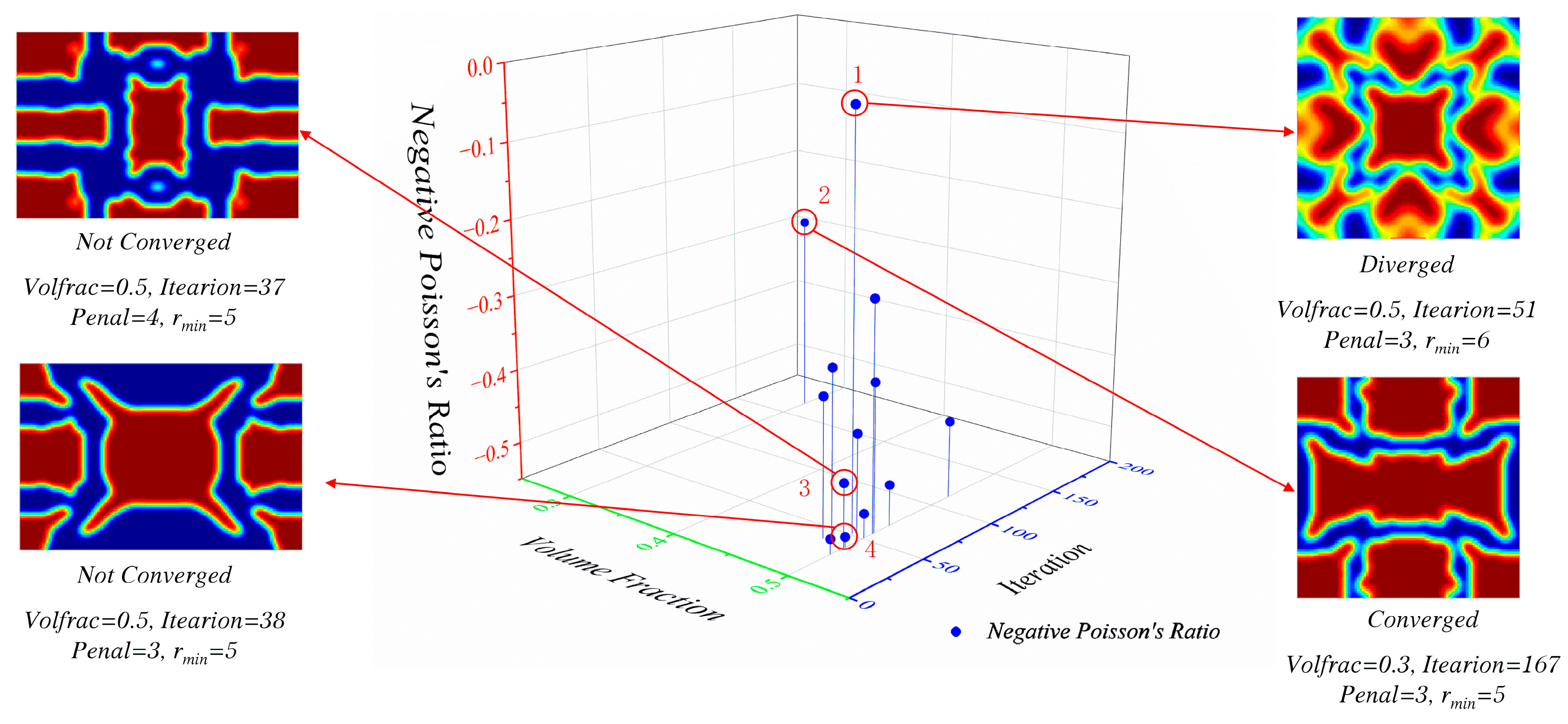
5.1. Analysis of Optimization Results and Iterative Process

Various single-cell optimization results were obtained under different sensitivity filtering radii, penalty factors, and volume fractions, and these results were plotted as a three-dimensional scatter plot, as depicted in Figure 5. The porous structure distribution was mainly affected by the penalty factor, where a large penalty factor resulted in slower flexibility changes, more iterations, and longer calculation times but better manufacturability. Moreover, a lower scatter point indicates a more pronounced negative Poisson’s ratio effect. Figure 6 portrays the iteration process of the objective function and the microstructure evolution during optimization. The historical curve indicates that although the maximum optimization step was set at 113, the primary topological configuration was essentially established at around 20 steps, highlighting the effectiveness of the method.

Figure 7 depicts the performance of negative Poisson’s ratio under different parameter combinations, along with the fluctuations in tolerance, namely sensitivity filtering radii, penalty factors, and volume fractions. It is observed that a well-formulated objective function can effectively guide the Poisson’s ratio of the structure to decrease rapidly, from around 0.3 to between −0.4 and −0.6 within the first 50 iterations, followed by a slow convergence. Simultaneously, the tolerance drops quickly and then oscillates around 0.1, as shown in Figure 7a–f. Some examples have undergone a second search, as depicted in Figure 7i. Examples that experience convergence difficulties often exhibit repeated tolerance oscillations, as observed in Figure 7a,b, which is attributed to the OC method’s simplicity and lack of robustness. To overcome this type of oscillation, which may impede convergence and decrease computational efficiency, other more robust optimizers such as MMA can be utilized. Examples that fail to converge generally employ sensitivity filtering methods or have improper parameter adjustments. Failure to converge is often manifested as an oscillation between two topological configurations at around 30 to 40 iterations, without a clear boundary evolution. Each iteration takes around 1.5 s, with a maximum total time of no more than 300 s (as shown in Figure 7d). Successful convergence examples were compared with commercial finite element software, revealing similar optimization processes that evolve the fundamental force transmission path, thereby verifying the method’s correctness and compactness.

The evolution results of 100 × 100 elements and their corresponding iteration steps, Poisson’s ratio, constrained volume fraction, and elastic matrix are summarized in

Table 1. Optimization results of a 100 × 100 unit under different parameters.

Pattern	Iteration Numbers	Volume Fraction	Poisson’s Ratio	Equivalent Elastic $\mathbf{Matrix} {\mathit{E}}^{\mathit{H}}$
	167	0.3	−0.2772	$\left(\begin{array}{ccc}0.0635& -0.0176& 0\\ -0.0176& 0.0096& 0\\ 0& 0& 0.0006\end{array}\right)$
	113	0.5	−0.4480	$\left(\begin{array}{ccc}0.0759& -0.0340& 0\\ -0.0340& 0.0759& 0\\ 0& 0& 0.0047\end{array}\right)$
	45	0.5	−0.3352	$\left(\begin{array}{ccc}0.0759& -0.0340& 0\\ -0.0340& 0.0549& 0\\ 0& 0& 0.0066\end{array}\right)$
	58	0.5	−0.3550	$\left(\begin{array}{ccc}0.0938& -0.0333& 0\\ -0.0333& 0.0938& 0\\ 0& 0& 0.0071\end{array}\right)$
	51	0.5	−0.5183	$\left(\begin{array}{ccc}0.0791& -0.0410& 0\\ -0.0410& 0.0791& 0\\ 0& 0& 0.0046\end{array}\right)$
*	51	0.5	−0.0173	$\left(\begin{array}{ccc}0.0347& -0.0006& 0\\ -0.0006& 0.0347& 0\\ 0& 0& 0.0036\end{array}\right)$

* A typical example of convergence failure.

. The evolution results of 150 × 100 elements and their corresponding iteration steps, Poisson’s ratio, constrained volume fraction, and elastic matrix are summarized in

Table 2. Optimization results of a 120 × 100 unit under different parameters.

Pattern	Iteration Numbers	Volume Fraction	Poisson’s Ratio	Equivalent Elastic $\mathbf{Matrix} {\mathit{E}}^{\mathit{H}}$
	46	0.5	−0.4109	$\left(\begin{array}{ccc}0.1173& -0.0482& 0\\ -0.0482& 0.0469& 0\\ 0& 0& 0.0050\end{array}\right)$
	57	0.5	−0.2498	$\left(\begin{array}{ccc}0.1605& -0.0401& 0\\ -0.0401& 0.0196& 0\\ 0& 0& 0.0028\end{array}\right)$
	37	0.5	−0.4665	$\left(\begin{array}{ccc}0.1194& -0.0557& 0\\ -0.0557& 0.0757& 0\\ 0& 0& 0.0051\end{array}\right)$
	69	0.5	−0.4963	$\left(\begin{array}{ccc}0.1096& -0.0544& 0\\ -0.0544& 0.0764& 0\\ 0& 0& 0.0072\end{array}\right)$
	28	0.5	−0.5301	$\left(\begin{array}{ccc}0.1047& -0.0555& 0\\ -0.0555& 0.0984& 0\\ 0& 0& 0.0073\end{array}\right)$
	38	0.5	−0.5367	$\left(\begin{array}{ccc}0.0790& -0.0424& 0\\ -0.0424& 0.0622& 0\\ 0& 0& 0.0024\end{array}\right)$

. By observing the Poisson’s ratio optimization results, it can be seen that the negative Poisson’s ratio effect is evident in both cases, with a maximum of −0.5183 for 100 × 100 elements and 150 × 100 elements. The last row of Table 1 is a typical example of convergence failure, which indicates that successful cases generally have clear manufacturable boundaries and significant negative Poisson’s ratio results. Accurate optimization parameter tuning is usually required; otherwise, such ambiguous boundaries and a Poisson’s ratio approaching zero may occur. Furthermore, it is common for prosperous instances to showcase intriguing traits, such as re-entrant or chiral characteristics, as evidenced by rows 6 and 3 of Table 2. These two kinds of distortions have been extensively established in previous research as the two configurations that attain the most negative Poisson’s ratios. Moreover, there exist configurations that blend both concave and chiral traits, as demonstrated in rows 2, 4, and 5 of Table 2. Nevertheless, the Poisson’s ratios achieved by topological optimization transcend the limits of conventional forward design.

It should be noted that the optimization process is based on the calculation results of the strain field, and thus the shape of the evolution of negative Poisson’s ratio has no direct relationship with the elastic modulus of the solid material. Therefore, the elastic modulus of the material is assigned as 1. However, the effective elastic modulus $E^H$ is directly related to the material’s elastic modulus, and thus $E^H$ here can only represent the equivalent situation of materials with an elastic modulus of 1, which has no practical significance. In experiments, the material’s elastic modulus should be obtained by nano-indentation on the sample, and the calculation of the homogenization matrix would be meaningful for the equivalent constitutive parameters.

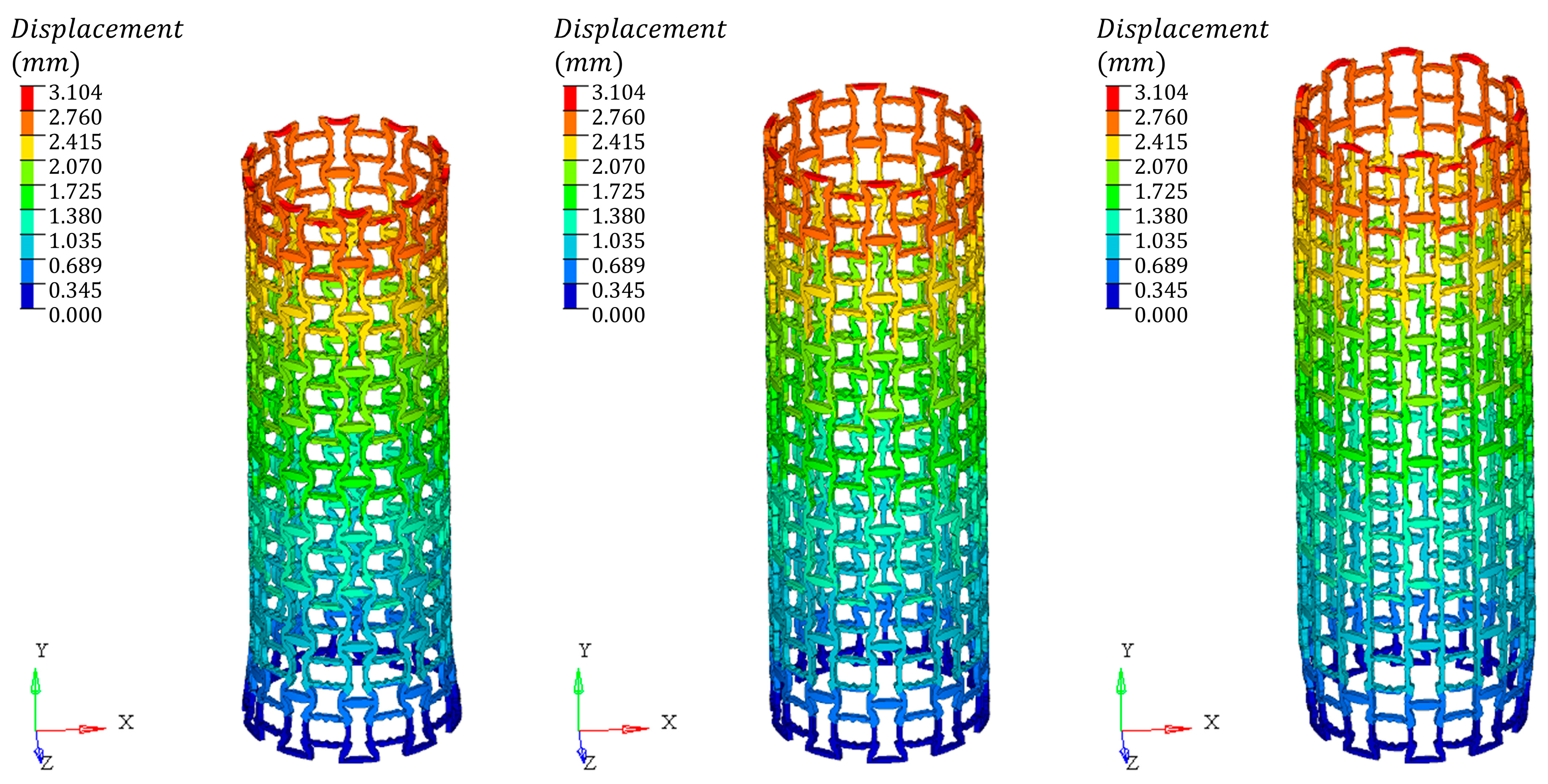
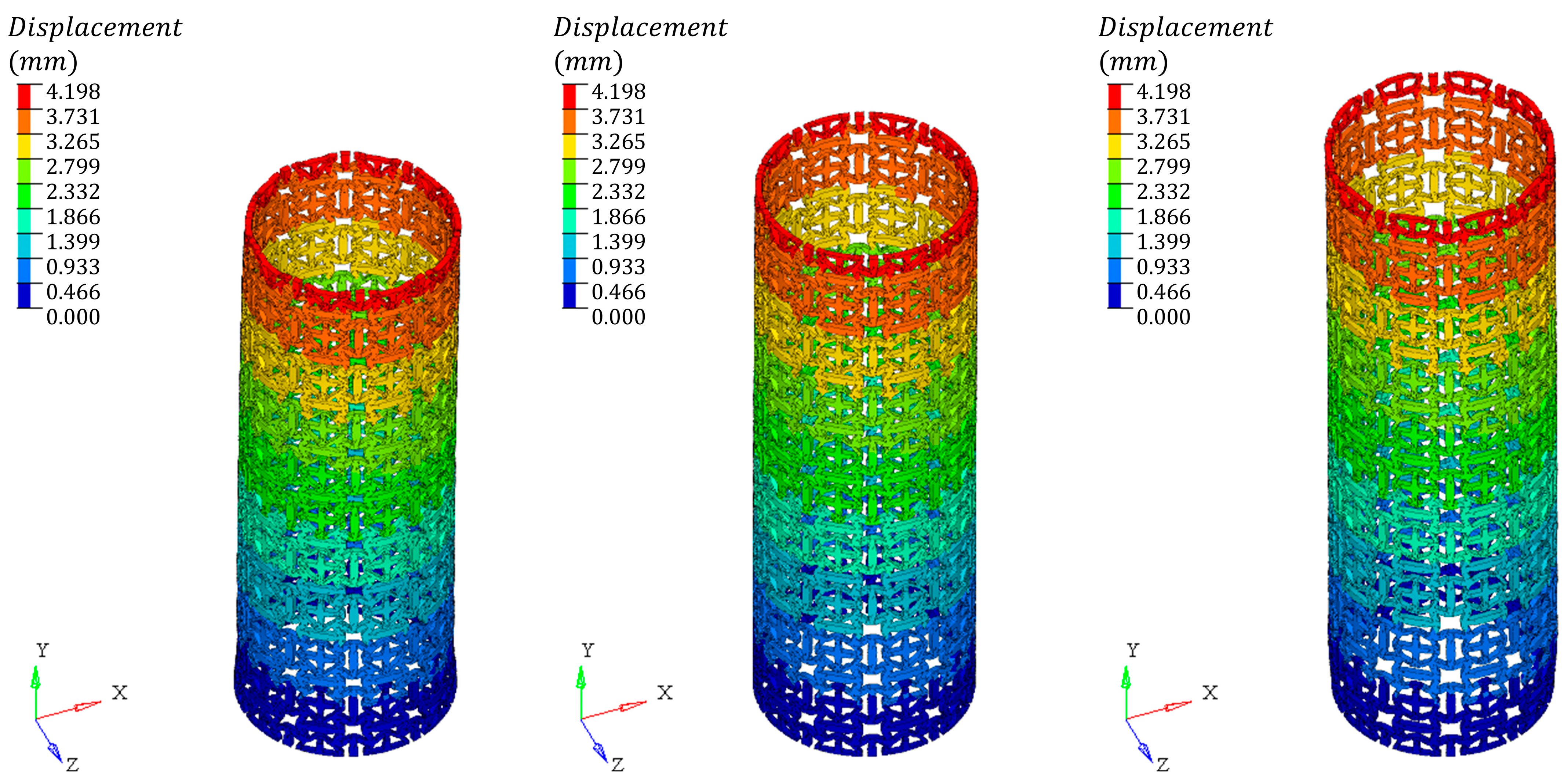
5.2. Finite Element Simulation Verification

Four types of cells with significant negative Poisson’s ratio effects were selected for finite element analysis. The optimized boundary shape of the cells was drawn in CAD in sizes of 5 mm × 5 mm and 5 mm × 7.5 mm and further imported into UG 11.0 to generate stacked tubular cell models using surface sheet metal functions. The overall size of the models was approximately 5 mm, and the modeling process is shown in Figure 8a. SHELL elements with a thickness of 0.5 mm were used for the cells, and a tetrahedral–hexahedral hybrid mesh was applied. The four models were, respectively, divided into 205,110 nodes and 215,914 elements, 128,410 nodes and 109,440 elements, 243,256 nodes and 308,190 elements, and 253,253 nodes and 285,200 elements. A mesh inspection showed good quality without significant warping or skewness, with a minimum Jacobian value of no less than 0.7 and a maximum aspect ratio no higher than 5.

To establish tension and compression conditions, a uniform axial force of 50 N was applied to all nodes on the top end face, while the freedom of all nodes on the bottom end face was constrained. The material properties were determined by importing the tensile curve of the 316L standard specimen prepared by selective laser melting into the finite element analysis software Hypermesh, as shown in Figure 8b. The material was found to be a typical elastic–plastic material with linear strain hardening behavior and an elastic modulus E of 196,000 MPa, Poisson’s ratio μ of 0.3, a yield stress of 205 MPa, and a limit stress of 515 MPa at 60% plastic deformation. To input the material density, the Archimedes drainage method was used to measure the density η of the 316L cube specimen prepared by selective laser melting. The specimen was polished and cleaned with ultrasonic water-free ethanol and the mass was measured using a high-precision balance. The density η was calculated as follows:

$$\eta =\frac{m_1\times {\rho }_0}{m_1-m_2}\times \frac{1}{{\rho }_1}\times 100\mathrm{\%}$$

(21)

where $m_1$ is the mass of the specimen exposed to air, $m_2$ is the mass of the specimen immersed in water, and ${\rho }_0$ is the density of deionized water, which is 998.2 kg/m³. The average of six experiments yielded a specimen density $\eta$ of 99.6%; thus, the density can be approximated by the theoretical value of 7.98 × 10⁻⁹ g/mm³ for 316L.

The finite element analysis results shown in Figure 9, Figure 10, Figure 11, and Figure 12, respectively, demonstrate the deformation behavior of four types of negative Poisson’s ratio lattice structures under both tensile and compressive loading conditions. Among them, the axial strain in Figure 9 is 0.031, the axial strain in Figure 10 is 0.087, the axial strain in Figure 11 is 0.065, and the axial strain in Figure 12 is 0.042. It is evident that the tensile–compressive behavior of the negative Poisson’s ratio has been achieved, with the compressed models exhibiting radial contraction on the left and the stretched models exhibiting radial expansion on the right. Such unique expansive deformation performance can be further applied in structures requiring self-expansion, such as vascular stents, or as a deformation compensation method for zero thermal expansion structures, with significant potential for practical applications. Of note, the structures represented by Figure 9 and Figure 10 exhibit significant deformation imbalance under large deformation. Regardless of compression or tension, the deformation at the ends is always greater than that in the middle, which is colloquially known as the “dog bone phenomenon” in the unfolding of heart stents, which may cause undue damage to the arterial wall. Conversely, in Figure 11 and Figure 12, it is evident that the tubular structures maintain uniform deformation even under large deformation. This performance is particularly prominent in Figure 12 and holds great promise for practical applications.

Since the tensile curve contains failure information, the failure nodes could be selected by observing the static analysis results, as shown in Figure 13. The failure nodes were mainly distributed at the weak connections of the rod, but no obvious stress concentration was observed, which could indirectly verify the rationality of the design method. Based on the static linear analysis, the structure shown in Figure 12 was perturbed to analyze its first buckling mode, as shown in Figure 14. It could be seen that the buckling of this lattice structure is mainly characterized by the inward folding of the end face. Unlike conventional modal analysis, for the modal analysis of instability, only the first-order vibration mode is observed. This is because the structure is considered to have failed once instability occurs for the first time.

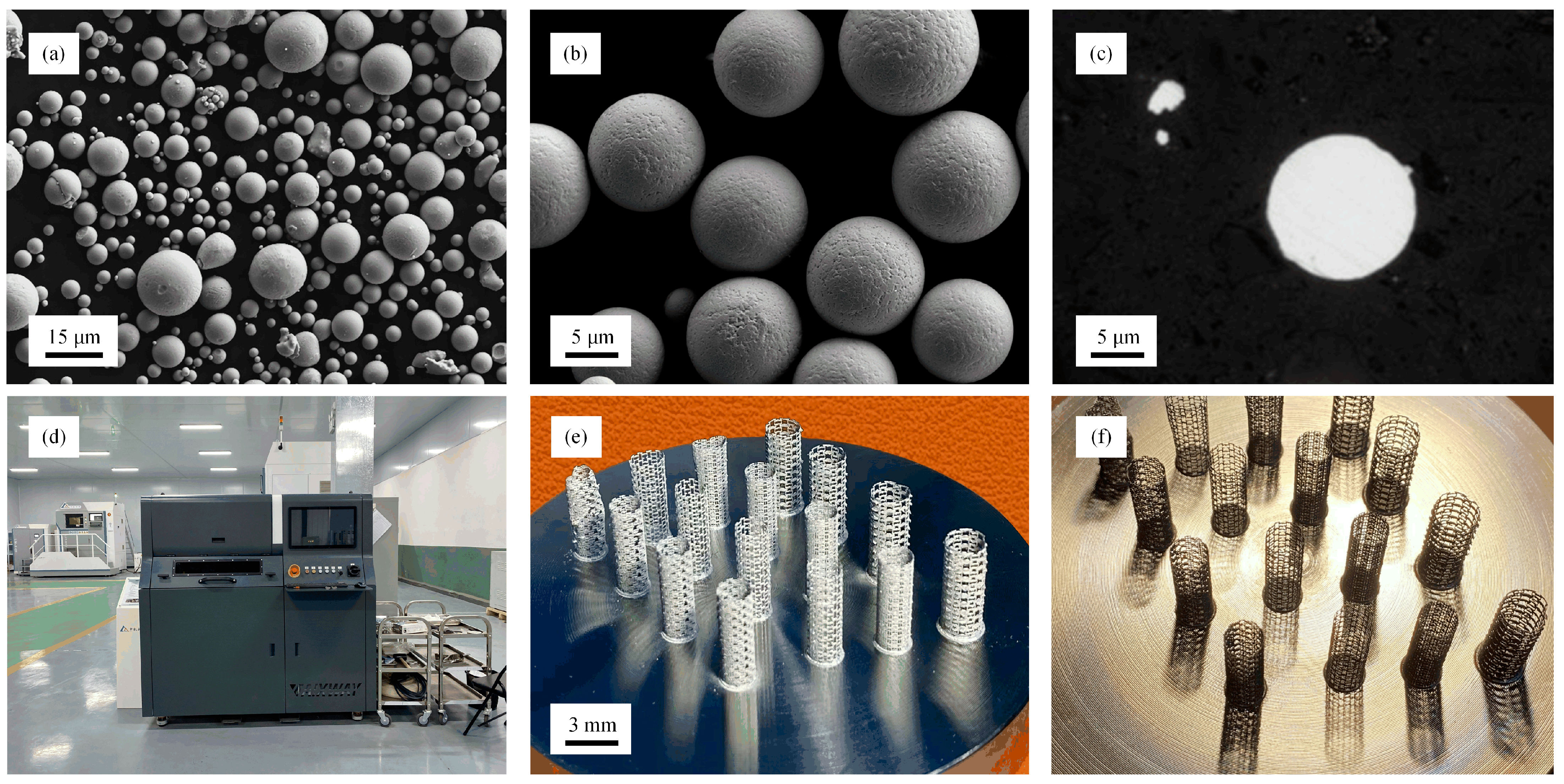
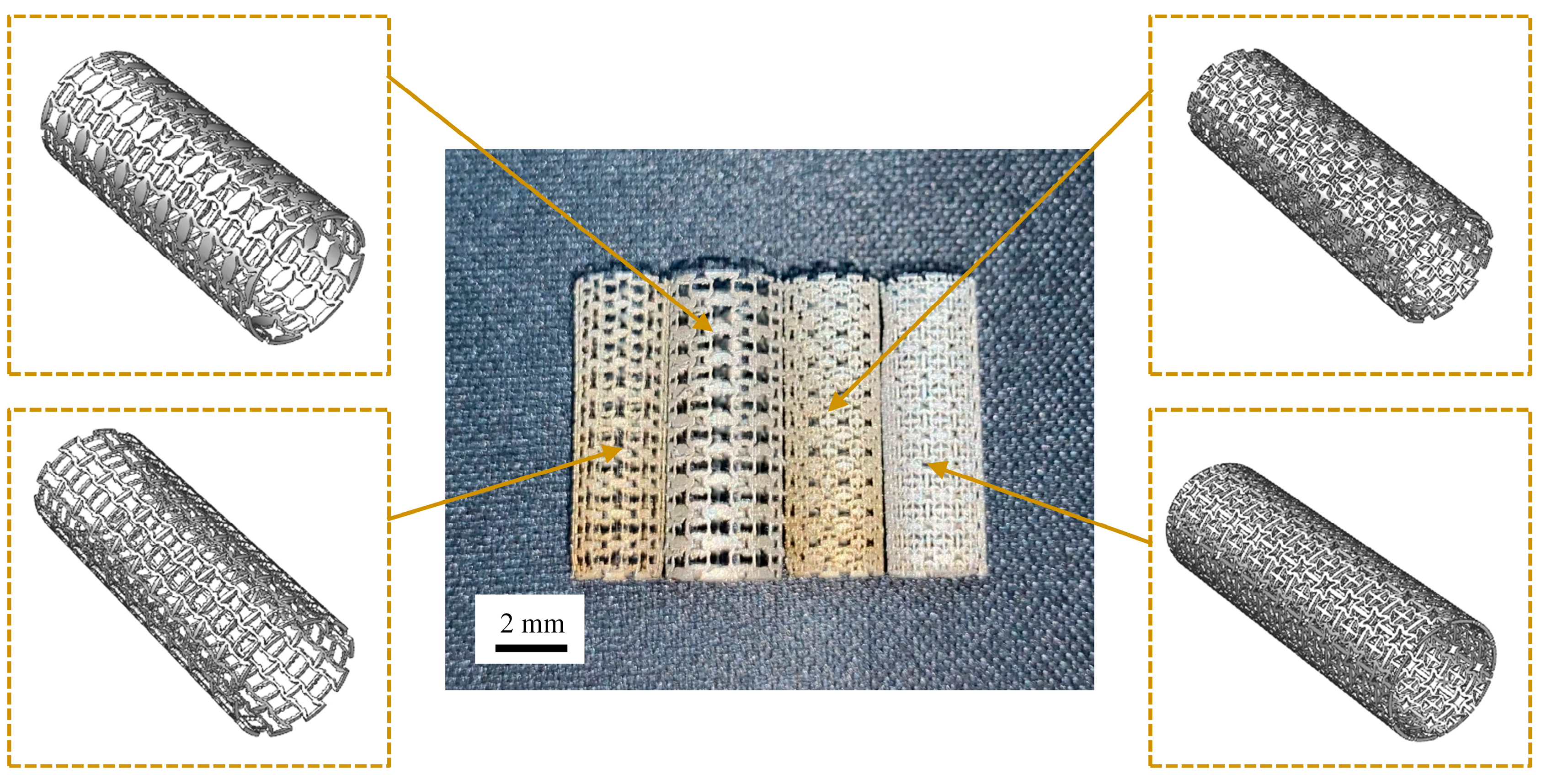
5.3. Microscale Laser Additive Manufacturing

The four tubular structures previously mentioned were fabricated as small-scale samples utilizing a microscale selective laser melting (SLM) process and 316L stainless steel powder. The success of printing and the performance of components in SLM are directly influenced by the quality of the powder used [32]. The factors that affect powder quality include powder sphericity, surface morphology, particle size distribution, and alloy element content. To achieve high relative density and mechanical properties in powder bed 3D printing, good powder flowability is essential, which is impacted by several factors such as sphericity, surface defects, and humidity. In a study by Sun et al. [33], the “sphericity factor” of powders was found to decrease as printing times increased, resulting in increased inter-particle friction and decreased powder flowability. To minimize friction between powder particles and achieve optimal flowability, highly spherical, smooth, and dry powders were necessary. Furthermore, the particle size distribution of the powder significantly affects the printed component’s relative density, surface roughness, and mechanical properties. Matching the powder size distribution reasonably can effectively improve the quality of the printed components. Attar et al. [34] found that specimens printed with nearly spherical mixed powders had significantly improved relative density and compression elongation compared to those printed with irregular powders when using MTT SLM250 HL equipment to prepare TiB-reinforced titanium-based composites. This is because, under loading conditions, stress is easily concentrated at the sharp interfaces between reinforcement particles and the matrix, forming cracks and causing the particle reinforcement effect to fail. Nearly spherical particles have smoother interfaces with the matrix and are less prone to stress concentration, resulting in higher strength and elongation. Powder particle size distribution is also closely related to laser absorption, material flow in the melt pool, and heat transfer in the powder bed. A study by Lee and Zhang [35] found that coarse-particle powders have more significant fluctuations in the melt pool edge shape than small-particle powders under laser irradiation, resulting in an irregular melt pool and a rough surface of the printed components. The phenomenon of melt pool “balling” may even occur during the printing process, leading to cracking and printing failure.

Furthermore, suitable pre-treatment methods and process parameters can enhance the quality of SLM-manufactured 316L stainless steel components [36]. Reference [37] suggested that the use of appropriate laser power and scanning speed can ensure the manufacturing of high-density 316L stainless steel parts while concurrently mitigating the occurrence of microstructural flaws.

The utilized process parameters included a powder layer thickness of 0.01 mm, a laser power of 35 W, an inner filling scanning speed of 1000 mm/s, an outer contour scanning speed of 80 mm/s, a laser timing half-period of 11,490/64 μs, and a laser timing pulse length of 6400/64 μs. The substrate material employed was 45# steel, while the powder material utilized was 316L stainless steel powder generated by gas atomization. The scanning electron microscopy (SEM) micrographs of the powder at various magnifications are presented in Figure 15a,b, displaying the sound sphericity of the powder particles. The cross-sectional SEM micrograph of the powder is shown in Figure 15c, which exhibits excellent compactness. This observation further corroborates the previously measured 99.6% compactness value. The median particle diameter D₅₀ was determined to be 10.05 μm, and the volume average diameter was 10.09 μm, satisfying the requirements of microscale printing. The chemical composition of 316L stainless steel powder is shown in

Table 3. The chemical composition of 316L stainless steel powder.

Composition	C	Si	Mn	P	S	Cr	Ni	Mo	Fe
Requirements of GB	≤0.03	≤1.00	≤2.00	≤0.035	≤0.03	16.0–18.0	10.0–14.0	2.0–3.0	Bal.
Measured contents	-	0.525	1.2	0.025	-	16.9	10.6	2.4	Bal.

. The experimental apparatus employed was the Precision-100 microscale selective laser melting equipment, jointly developed by the China Academy of Machinery Science and Technology and the Fraunhofer Institute for Laser Technology in Germany. The device also marks the first microscale selective laser melting equipment in China, as shown in Figure 15d.

Table 4. Aixway Precision-100 microscale 3D printer device parameters.

Parameters	Values
Building volume (Ø × H)	100 × 100 mm
Layer thickness	1–15 μm
Laser type	200 W Yb-fiber laser
Focus diameter	<25 μm
Scanning speed	max. 3 m/s
Surface roughness	min. Sa 1 μm
Powder size distribution	2–10 µm
Accuracy	<30 µm
Shielding gases	Nitrogen, argon

lists the device parameters. The prepared samples are depicted in Figure 15e and were completed in approximately 12 h. The printing outcomes, as depicted in Figure 15f, exhibit commendable transparency, along with a height of 5 mm. Additionally, the printed structure manifests a precise reconstruction of the design features, well-defined contours, rapid printing velocity, and a complete absence of any auxiliary supports, as shown in Figure 16.

5.4. Quasi-Static Compression

The experimental verification of the collapse and negative Poisson’s ratio effect was performed on a TCD-C-2000N high-precision spring tester. A cylindrical loading head was used to push the sample from the top surface in the height direction (i.e., axial direction). The loading force was set to 50 N, and the loading speed was set to 1 mm/min, which also meant a strain rate of 1.04 to ensure quasi-static loading conditions. To ensure the elastic stage was fully recorded, the maximum deformation of the loading head was first set to 0.3 mm, i.e., an axial strain of 0.06, and then continued to compress until the collapse occurred.

The motion was recorded using a high-resolution industrial camera (IDS Imaging Development Systems GmbH) at a rate of approximately 60 frames per second. Load–time and displacement–time curves were output to obtain the load–displacement curve, with a sampling frequency of 10 Hz.

Based on the finite element analysis results from earlier, the Poisson’s ratio of −0.4480 design with the best stability was selected. Photos of the initial state and the end of the elastic stage were taken with 50% transparency and overlaid to ensure that the left and right edges of the loading head and the test bench were aligned. The red dashed box in Figure 17a shows the initial and final states of the elastic stage deformation of the tubular structure. It can be seen that under axial compression, the tubular structure underwent radial contraction, which is consistent with the results shown in Figure 12. The negative Poisson’s ratio effect and the accuracy of the finite element analysis have been fully verified. Observing the sample in Figure 17b, its end deformation form is in complete agreement with the first buckling mode shape shown in Figure 13, manifested as inward folding, which validates the correctness of the buckling analysis on the lateral side. Furthermore, the collapse of the structure occurred at a load of approximately 40 N, indicating that its strength is lower compared to forged steel.

6. Conclusions

• Based on the energy homogenization method and SIMP topology optimization method, a relaxed objective function was proposed and the damping in the optimization criterion was removed to achieve negative Poisson’s ratio lattice cells;
• Optimization calculations yield multiple sets of negative Poisson’s ratio unit cells, with the lowest Poisson’s ratio achieving −0.5367, and an equivalent elastic matrix was derived. The iterative process’s efficiency is comparable to that of commercial software, with a maximum iteration time of 300 s, enabling the prompt identification of fundamental configurations;
• The validity of the proposed method was verified through the finite element analysis of four tubular structures, revealing distinct auxetic deformation patterns and inward folding buckling forms;
• Tubular samples of 5 mm made of 316L stainless steel were successfully fabricated using the microscale selective laser melting, with adequate printing precision and sound feature reproduction. The process demonstrated that a set of parameters, comprising a powder layer thickness of 0.01 mm, a laser power of 35 W, an inner filling scanning speed of 1000 mm/s, and an outer contour scanning speed of 80 mm/s, can enable the successful additive manufacturing of a metallic coronary stent according to the prescribed scale of application. Quasi-static compression experiments showed negative Poisson’s ratio effects and buckling forms that align with finite element analysis results, verifying the method’s correctness.
• Quasi-static compression experiments showed negative Poisson’s ratio effects and buckling forms that align with finite element analysis results, verifying the method’s correctness.

Although the algorithm proposed in this paper is characterized by its compactness and simplicity, it has proven to be less robust than desired. In light of this, future studies may consider incorporating other optimizers, such as MMA or GCMMA, in order to enhance the algorithm’s resilience. Additionally, the conclusions derived from the 2D image optimization method could potentially be extended to 3D structures. Furthermore, by introducing aggregate functions, the single-objective single-constraint optimization method may be extended to multi-objective topology optimization, thus broadening the scope of this approach and unlocking its potential in various fields, including but not limited to coronary stents, esophageal stents, helmets, protective equipment, bullets, and beyond.

References

1. Kolpakov, A.G. Determination of the Average Characteristics of Elastic Frameworks. J. Appl. Math. Mech. 1985, 49, 739–745. [Google Scholar] [CrossRef]
2. Saxena, K.K.; Das, R.; Calius, E.P. Three Decades of Auxetics Research—Materials with Negative Poisson’s Ratio: A Review. Adv. Eng. Mater. 2016, 18, 1847–1870. [Google Scholar] [CrossRef]
3. Vasil’ev, V.V.; Lurie, S.A. Generalized theory of elasticity. Mech. Sol. 2015, 50, 379–388. [Google Scholar] [CrossRef]
4. Lakes, R. Foam Structures with a Negative Poissons Ratio. Science 1987, 235, 1038–1040. [Google Scholar] [CrossRef] [PubMed]
5. Mizzi, L.; Attard, D.; Gatt, R.; Farrugia, P.S.; Grima, J.N. An analytical and finite element study on the mechanical properties of irregular hexachiral honeycombs. Smart Mater. Struct. 2018, 27, 11. [Google Scholar] [CrossRef]
6. Mizzi, L.; Attard, D.; Gatt, R.; Pozniak, A.A.; Wojciechowski, K.W.; Grima, J.N. Influence of translational disorder on the mechanical properties of hexachiral honeycomb systems. Compos. Part B Eng. 2015, 80, 84–91. [Google Scholar] [CrossRef]
7. Pozniak, A.A.; Wojciechowski, K.W. Poisson’s ratio of rectangular anti-chiral structures with size dispersion of circular nodes. Phys. Status Solidi B Basic Solid State Phys. 2014, 251, 367–374. [Google Scholar] [CrossRef]
8. Idczak, E.; Strek, T. Minimization of Poisson’s ratio in anti-tetra-chiral two-phase structure. IOP Conf. Ser. Mater. Sci. Eng. 2017, 248, 012006. [Google Scholar] [CrossRef]
9. Zhang, H.K.; Luo, Y.J.; Kang, Z. Bi-material microstructural design of chiral auxetic metamaterials using topology optimization. Compos. Struct. 2018, 195, 232–248. [Google Scholar] [CrossRef]
10. Zarrinmehr, S.; Ettehad, M.; Kalantar, N.; Borhani, A.; Sueda, S.; Akleman, E. Interlocked archimedean spirals for conversion of planar rigid panels into locally flexible panels with stiffness control. Comput. Graph. 2017, 66, 93–102. [Google Scholar] [CrossRef]
11. Novak, N.; Vesenjak, M.; Ren, Z. Auxetic Cellular Materials—A Review. Strojniski Vestn. J. Mech. Eng. 2016, 62, 485–493. [Google Scholar] [CrossRef]
12. Ha, C.S.; Plesha, M.E.; Lakes, R.S. Chiral three-dimensional lattices with tunable Poisson’s ratio. Smart Mater. Struct. 2016, 25, 6. [Google Scholar] [CrossRef]
13. Duan, S.Y.; Wen, W.B.; Fang, D.N. A predictive micropolar continuum model for a novel three-dimensional chiral lattice with size effect and tension-twist coupling behavior. J. Mech. Phys. Solids 2018, 121, 23–46. [Google Scholar] [CrossRef]
14. Clausen, A.; Wang, F.W.; Jensen, J.S.; Sigmund, O.; Lewis, J.A. Topology Optimized Architectures with Programmable Poisson’s Ratio over Large Deformations. Adv. Mater. 2015, 27, 5523–5527. [Google Scholar] [CrossRef] [PubMed]
15. Wang, F.W. Systematic design of 3D auxetic lattice materials with programmable Poisson’s ratio for finite strains. J. Mech. Phys. Solids 2018, 114, 303–318. [Google Scholar] [CrossRef]
16. McCaw, J.C.S.; Cuan-Urquizo, E. Curved-Layered Additive Manufacturing of non-planar, parametric lattice structures. Mater. Des. 2018, 160, 949–963. [Google Scholar] [CrossRef]
17. Wang, T.; Wang, L.M.; Ma, Z.D.; Hulbert, G.M. Elastic analysis of auxetic cellular structure consisting of re-entrant hexagonal cells using a strain-based expansion homogenization method. Mater. Des. 2018, 160, 284–293. [Google Scholar] [CrossRef]
18. Beharic, A.; Egui, R.R.; Yang, L. Drop-weight impact characteristics of additively manufactured sandwich structures with different cellular designs. Mater. Des. 2018, 145, 122–134. [Google Scholar] [CrossRef]
19. Yuan, S.Q.; Shen, F.; Bai, J.M.; Chua, C.K.; Wei, J.; Zhou, K. 3D soft auxetic lattice structures fabricated by selective laser sintering: TPU powder evaluation and process optimization. Mater. Des. 2017, 120, 317–327. [Google Scholar] [CrossRef]
20. Ingrole, A.; Hao, A.; Liang, R. Design and modeling of auxetic and hybrid honeycomb structures for in-plane property enhancement. Mater. Des. 2017, 117, 72–83. [Google Scholar] [CrossRef]
21. Hou, S.Y.; Li, T.T.; Jia, Z.; Wang, L.F. Mechanical properties of sandwich composites with 3d-printed auxetic and non-auxetic lattice cores under low velocity impact. Mater. Des. 2018, 160, 1305–1321. [Google Scholar] [CrossRef]
22. Li, T.T.; Chen, Y.Y.; Hu, X.Y.; Li, Y.B.; Wang, L.F. Exploiting negative Poisson’s ratio to design 3D-printed composites with enhanced mechanical properties. Mater. Des. 2018, 142, 247–258. [Google Scholar] [CrossRef]
23. Xiong, J.P.; Gu, D.D.; Chen, H.Y.; Dai, D.H.; Shi, Q.M. Structural optimization of re-entrant negative Poisson’s ratio structure fabricated by selective laser melting. Mater. Des. 2017, 120, 307–316. [Google Scholar] [CrossRef]
24. Andreassen, E.; Clausen, A.; Schevenels, M.; Lazarov, B.S.; Sigmund, O. Efficient topology optimization in MATLAB using 88 lines of code. Struct. Multidiscip. Optim. 2011, 43, 1–16. [Google Scholar] [CrossRef]
25. Zhang, S.; Li, H.; Huang, Y. An improved multi-objective topology optimization model based on SIMP method for continuum structures including self-weight. Struct. Multidiscip. Optim. 2021, 63, 211–230. [Google Scholar] [CrossRef]
26. Bendse, M.; Sigmund, O. Topology Optimization: Theory, Method and Applications; Springer Science & Business Media: Berlin, Germany, 2003. [Google Scholar]
27. Yin, L.Z.; Yang, W. Optimality criteria method for topology optimization under multiple constraints. Comput. Struct. 2001, 79, 1839–1850. [Google Scholar] [CrossRef]
28. Svanberg, K. The Method of Moving Asymptotes—A New Method for Structural Optimization. Int. J. Numer. Methods Eng. 1987, 24, 359–373. [Google Scholar] [CrossRef]
29. Wang, Y.Q.; Luo, Z.; Zhang, N.; Kang, Z. Topological shape optimization of microstructural metamaterials using a level set method. Comput. Mater. Sci. 2014, 87, 178–186. [Google Scholar] [CrossRef]
30. Wang, M.Y.; Wang, X.M.; Guo, D.M. A level set method for structural topology optimization. Comput. Meth. Appl. Mech. Eng. 2003, 192, 227–246. [Google Scholar] [CrossRef]
31. Allaire, G.; Jouve, F.; Toader, A.M. Structural optimization using sensitivity analysis and a level-set method. J. Comput. Phys. 2004, 194, 363–393. [Google Scholar] [CrossRef]
32. Hu, Q.P.; Wang, M.H.; Chen, Y.B.; Liu, H.L.; Si, Z. The Effect of MC-Type Carbides on the Microstructure and Wear Behavior of S390 High-Speed Steel Produced via Spark Plasma Sintering. Metals 2022, 12, 2168. [Google Scholar] [CrossRef]
33. Sun, Y.Y.; Gulizia, S.; Oh, C.H.; Doblin, C.; Yang, Y.F.; Qian, M. Manipulation and Characterization of a Novel Titanium Powder Precursor for Additive Manufacturing Applications. JOM 2015, 67, 564–572. [Google Scholar] [CrossRef]
34. Attar, H.; Prashanth, K.G.; Zhang, L.C.; Calin, M.; Okulov, I.V.; Scudino, S.; Yang, C.; Eckert, J. Effect of Powder Particle Shape on the Properties of In Situ Ti-TiB Composite Materials Produced by Selective Laser Melting. J. Mater. Sci. Technol. 2015, 31, 1001–1005. [Google Scholar] [CrossRef]
35. Lee, Y.S.; Zhang, W. Mesoscopic simulation of heat transfer and fluid flow in laser Powder bed additive manufacturing. In Proceedings of the 26th Solid Freeform Fabrication Symposium, Austin, TX, USA, 10–12 August 2015. [Google Scholar]
36. Yang, D.C.; Kan, X.F.; Gao, P.F.; Zhao, Y.; Yin, Y.J.; Zhao, Z.Z.; Sun, J.Q. Influence of porosity on mechanical and corrosion properties of SLM 316L stainless steel. Appl. Phys. A Mater. Sci. Process. 2022, 128, 9. [Google Scholar] [CrossRef]
37. Ara, I.; Azarmi, F.; Tangpong, X.W. Microstructure Analysis of High-Density 316L Stainless Steel Manufactured by Selective Laser Melting Process. Metallogr. Microstruct. Anal. 2021, 10, 754–767. [Google Scholar] [CrossRef]
Figure 1. Flowchart of the numerical process to simulate structures with negative Poisson’s ratio.
Machines 11 00519 g001
Figure 2. The unit cell displacement field under the energy homogenization method.
Machines 11 00519 g002
Figure 3. The nomenclature for the macroscopic displacement field U in the case of a unit cell partitioned into a 3 × 3 array of elements.
Machines 11 00519 g003
Figure 4. Optimization result by directly treating the Poisson’s ratio in quotient form as the objective function.
Machines 11 00519 g004
Figure 5. Single-cell optimization results under different sensitivity filtering radii, penalty factors, and volume fractions.
Machines 11 00519 g005
Figure 6. A typical iterative process and tolerance fluctuation.
Machines 11 00519 g006
Figure 7. Iterative performance and tolerance variation under various parameter combinations, with the lowest Poisson’s ratio achieving (a) −0.3550; (b) −0.3352; (c) −0.5301; (d) −0.4665; (e) −0.4109; (f) −0.2772; (g) −0.5183; (h) −0.4963; (i) −0.5367.
Machines 11 00519 g007
Figure 8. (a) The finite element validation process for a typical unit cell based on a tubular structure. (b) The tensile curve for the standard 316L specimen.
Machines 11 00519 g008
Figure 9. The finite element analysis results of the compression and tension of a lattice structure designed with a Poisson’s ratio of −0.2772.
Machines 11 00519 g009
Figure 10. The finite element analysis results of the compression and tension of a lattice structure designed with a Poisson’s ratio of −0.5367.
Machines 11 00519 g010
Figure 11. The finite element analysis results of the compression and tension of a lattice structure designed with a Poisson’s ratio of −0.3550.
Machines 11 00519 g011
Figure 12. The finite element analysis results of the compression and tension of a lattice structure designed with a Poisson’s ratio of −0.4480.
Machines 11 00519 g012
Figure 13. The finite element analysis of the failure nodes in a tubular lattice structure.
Machines 11 00519 g013
Figure 14. The first buckling mode of tubular lattice structures.
Machines 11 00519 g014
Figure 15. (a) The SEM micrograph of the 316L powder; (b) the SEM micrograph of the surface morphology of the 316L powder; (c) the cross-sectional SEM micrograph of the 316L powder; (d) Aixway Precision-100 microscale 3D printer; (e) the 5 mm sample fabricated by the microscale SLM process; (f) the transparency of the samples fabricated by the microscale SLM process.
Machines 11 00519 g015
Figure 16. Precise reconstruction of the design features through the microscale SLM process.
Machines 11 00519 g016
Figure 17. (a) The initial and final state photos of quasi-static elastic compression overlaid with 50% transparency; (b) the specimen after buckling failure.
Machines 11 00519 g017