A 3D Reduced Common Mode Voltage PWM Algorithm for a Five-Phase Six-Leg Inverter

Abstract

Neutral point voltage control converters (NPVCC) are being considered for AC drive applications, where their additional degree of freedom can be used for different purposes, such as fault tolerance or common mode voltage (CMV) reduction. For every PWM-driven converter, the CMV is an issue that must be considered since it can lead to shaft voltages between rotor and stator windings, generating bearing currents that accelerate bearing degradation, and can also produce a high level of electromagnetic interference (EMI). In light of these considerations, in this paper a three-dimensional reduced common mode voltage PWM (3D RCMV-PWM) technique is proposed which effectively reduces CMV in five-phase six-leg NPVCCs. The mathematical description of both the converter and the modulation technique, in space-vector and carrier-based approaches, is included. Furthermore, the simulation and experimental analysis validate the CMV reduction capability in addition to the good behaviour in terms of the efficiency and harmonic distortion of the proposed RCMV-PWM algorithm.

1. Introduction

Multiphase electric drive systems are attracting more and more attention due to their superior characteristics when compared to traditional three-phase systems. Among these advantages, lower torque ripple, higher power density, reduced current per phase and inherent fault tolerance capability are highlighted [1,2]. In this sense, despite the proposal of several multiphase topologies, star-connected structures with an odd number of phases are preferred. More precisely, five-phase technology has been extensively used, since it provides a good trade-off between system complexity and fault tolerance [3,4]. Furthermore, the fault tolerance capability has led to the use of multiphase systems in motor drive applications in which safety is a critical requirement as in electric vehicles and more electric aircraft [5,6,7].

In addition to the traditional voltage source inverter (VSI), neutral point voltage control converters (NPVCC) have been proposed for motor drive applications, where the three-phase four-leg converter stands out [8,9,10]. Likewise, multilevel NPVCCs [11] and multiphase NPVCCs, as in [12] where a pole-phase modulated induction motor is driven by using three three-phase four-leg inverters, have been also considered for motor drive applications. Similarly, a five-phase six-leg variation (Figure 1), intended for switching power amplifiers for magnetic levitation bearing systems, is explored in [13,14].

The control over the neutral point voltage (N in Figure 1) releases the constraint that the sum of the stator currents is zero. Consequently, this converter has the ability to control unbalanced loads. Although this converter has some disadvantages, such as the need for the machine to have access to the neutral point, it also has significant advantages. For example, the control over the neutral point voltage offers an extra degree of freedom that can be used for different purposes, such as fault tolerance [15] and common mode voltage (CMV) reduction [16,17].

CMV is a serious concern when speaking about system reliability. This voltage is an unavoidable consequence in pulse-width modulated (PWM) power converters. In addition to damaging the electric machine bearings [18], the CMV produces undesirable electromagnetic interferences [19] and leakage currents that flow through the machine, destroying the stator winding insulation [20]. These damages are mainly caused due to the high $\raisebox{1ex}{$dv$}\!\left/ \!\raisebox{-1ex}{$dt$}\right.$ caused by the inverter commutations on the machine terminals, in addition to the high voltage amplitude of CMV [21]. Furthermore, these effects are expected to worsen as the use of WBG devices becomes more common [20].

Generating sinewaves using high-frequency PWM can lead to bearing damage caused by common-mode voltage (CMV) from the inverter. Specifically, the unbalanced phase voltages produced by the PWM algorithm driving the power devices result in CMV profiles with abrupt edges. Due to the parasitic capacitances and the high $\raisebox{1ex}{$dv$}\!\left/ \!\raisebox{-1ex}{$dt$}\right.$ values, a replica of the CMV forms appears in the shaft. This may exceed the dielectric breakdown voltage of the lubrication film inside the bearing, resulting in arcing discharge sparks between the bearing races in the form of ringing current pulses. This leads to pitting and fluting. Furthermore, these fast-switching CMV shapes also degrade the stator windings and can cause significant electromagnetic interferences (EMI). The entire process of generating CMV is explained in detail in [22].

In order to overcome these harmful effects, PWM algorithms provide a flexible and cost-effective solution. In this context, several reduced common mode voltage modulation techniques (RCMV-PWM) have been proposed, with the most well-known being AZS-PWM, NS-PWM, and RS-PWM. In addition to these algorithms, which were initially proposed for three-phase converters, other techniques have been proposed that reduce CMV in converters with control over the neutral point [23,24]. For instance, the authors of [16] propose a carrier-based modulation technique to eliminate the common-mode leakage current in transformerless photovoltaic systems. Similarly, ref. [25] takes advantage of the neutral point connection to mitigate the load neutral point voltage by means of a new space-vector-based modulation technique. On the other hand, ref. [26] proposes a modulation technique to suppress the CMV in hybrid grids. Moreover, the proposed modulation results in a marked reduction in the DC grid voltage oscillation. In [23], the well-known near-state PWM (NS-PWM) modulation, first proposed for three-phase inverters in [27], is extended to three-phase four-leg inverters. Likewise, the only three-dimensional space-vector (3D SV-PWM) for a five-phase six-leg converter is proposed in [28].

To fill this gap in the literature, this work proposes a three-dimensional RCMV-PWM (3D RCMV-PWM), based on the well known NS-PWM, to be applied in five-phase six-leg motor drive systems. The authors have chosen to follow the principles of the NS-PWM technique because, unlike AZS-PWM, it does not reverse the polarity of the current within a single commutation period. Additionally, it has a greater linear range than those algorithms based on RS-PWM. Most importantly, NS-PWM techniques are discontinuous, which allows reducing the switching losses of the converter. This is where NS-PWM is superior to AZS-PWM and RS-PWM. In this sense, the technical challenge of operating the suggested PWM method for a five-phase six-leg inverter is to reduce the common-mode voltage without worsening other features of the complete system, such as efficiency.

For that purpose, the proposed converter and CMV are first introduced in Section 2 and Section 3. Secondly, the 3D RCMV-PWM is explained in detail in Section 4. Then, the CMV of the proposed modulation is analysed thoroughly by simulation in Section 5. Lastly, experimental results are given in Section 6. In this section, the CMV reduction is verified, and the efficiency and total harmonic distortion parameters are discussed for five-phase six-leg converters.

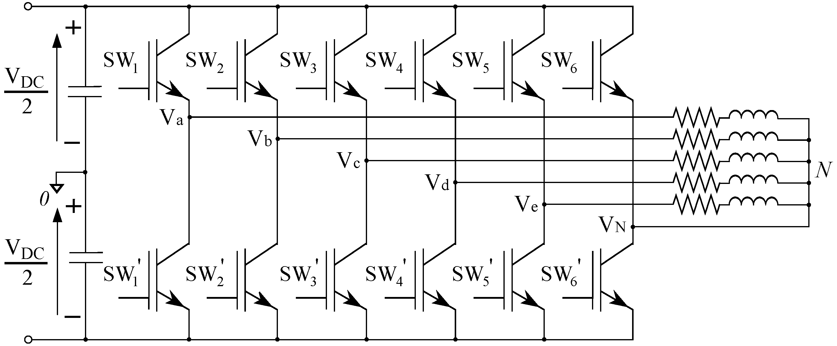
2. Five-Phase Six-Leg Vector Definition

Due to the control over the neutral point voltage, the space vector of a five-phase six-leg inverter is three-dimensional. Thus, the transition from $abcde$ coordinates to $\alpha \beta$xy$\gamma$ coordinates is expressed as

$$\left[V_{\alpha }{V}_{\beta }{V}_x{V}_y{V}_{\gamma }\right]=C_T\left[V_{aN}{V}_{bN}{V}_{cN}{V}_{dN}{V}_{eN}\right],$$

(1)

where $V_{iN}$ ($i\in a,b,c,d,e$) are the $abcde$ axis phase-to-neutral voltages (Figure 1):

$$\left[\begin{array}{c}{V}_{aN}\\ V_{bN}\\ V_{cN}\\ V_{dN}\\ V_{eN}\end{array}\right]=\left[\begin{array}{cccccc}1& 0& 0& 0& 0& -1\\ 0& 1& 0& 0& 0& -1\\ 0& 0& 1& 0& 0& -1\\ 0& 0& 0& 1& 0& -1\\ 0& 0& 0& 0& 1& -1\end{array}\right]\left[\begin{array}{c}{V}_{a0}\\ V_{b0}\\ V_{c0}\\ V_{d0}\\ V_{e0}\\ V_{N0}\end{array}\right],$$

(2)

where phase voltages are equal to $V_{i0}=(2S{W}_j-1)\raisebox{1ex}{$V_{DC}$}\!\left/ \!\raisebox{-1ex}{$2$}\right.$ and $S{W}_j$ ($j\in [1-6]$) equals 1 when the switch is active and 0 when the switch is inactive; $V_k$ ($k\in \alpha ,\beta ,x,y,\gamma$) are the voltage vector components and $C_T$ is the Clarke transformation matrix given by [28]:

$$C_T=\frac{2}{5}\left[\begin{array}{ccccc}1& cos\left({\displaystyle \frac{2\pi }{5}}\right)& cos\left({\displaystyle \frac{4\pi }{5}}\right)& cos\left({\displaystyle \frac{6\pi }{5}}\right)& cos\left({\displaystyle \frac{8\pi }{5}}\right)\\ 0& sin\left({\displaystyle \frac{2\pi }{5}}\right)& sin\left({\displaystyle \frac{4\pi }{5}}\right)& sin\left({\displaystyle \frac{6\pi }{5}}\right)& sin\left({\displaystyle \frac{8\pi }{5}}\right)\\ 1& cos\left({\displaystyle \frac{4\pi }{5}}\right)& cos\left({\displaystyle \frac{8\pi }{5}}\right)& cos\left({\displaystyle \frac{12\pi }{5}}\right)& cos\left({\displaystyle \frac{16\pi }{5}}\right)\\ 0& sin\left({\displaystyle \frac{4\pi }{5}}\right)& sin\left({\displaystyle \frac{8\pi }{5}}\right)& sin\left({\displaystyle \frac{12\pi }{5}}\right)& sin\left({\displaystyle \frac{16\pi }{5}}\right)\\ 0.5& 0.5& 0.5& 0.5& 0.5\end{array}\right].$$

(3)

The vector space of five-phase systems consists of two subspaces: $\alpha \beta$ and $xy$. When adding the sixth leg capable of defining the neutral point voltage, it is necessary to add a third dimension ($\gamma$) to each of these subspaces. Thus, the three-dimensional subspaces $\alpha \beta \gamma$ and $xy\gamma$ are defined. The vector space of a five-phase converter has the shape of a decagon, so adding a third dimension gives a decagonal prism. From here on, the $\alpha \beta \gamma$ decagonal prism will be taken as a reference. In this sense, Figure 2 shows the $\alpha \beta \gamma$ prism decomposed according to the values obtained by the $\gamma$ variable. This Figure shows all the vectors that make up the vector space, whose names are given by converting the first five-leg switching states, treated as a binary number, to decimals. The sixth branch switching state equals P (positive) when its value is 1 and N (negative) when its value is 0.

3. CMV Definition and Figures of Merit

The CMV can be defined as the mean value of the voltage difference between each phase and the reference point. Accordingly, the CMV equation for a five-phase six-leg converter has been derived from [23]:

$$v_{CMV}={\displaystyle \frac{v_{a0}+v_{b0}+v_{c0}+v_{d0}+v_{e0}+v_{N0}}{6}}.$$

(4)

In this way, it is possible to relate the converter switching states to the different CMV levels:

$$v_{CMV}=V_{DC}{\displaystyle \frac{S{W}_1+S{W}_2+S{W}_3+S{W}_4+S{W}_5+S{W}_6-3}{6}}.$$

(5)

For a better understanding,

Table 1. CMV levels of five-phase six-leg converter.

Switching-Vector	CMV Level
31P	$V_{DC}/2$
31N, 30P, 29P, 27P, 23P, 15P	$V_{DC}/3$
30N, 29N, 28P, 27N, 26P, 25P, 23N, 22P	$V_{DC}/6$
21P, 19P, 15N, 14P, 13P, 11P, 7P
28N, 26N, 25N, 24P, 22N, 21N, 20P, 19N
18P, 17P, 14N, 13N, 12P, 11N, 10P, 9P	0
7N, 6P, 5P, 3P
24N, 20N, 18N, 17N, 16P, 12N, 10N, 9N	$-V_{DC}/6$
8P, 6N, 5N, 4P, 3N, 2P, 1P
16N, 8N, 4N, 2N, 1N, 0P	$-V_{DC}/3$
0N	$-V_{DC}/2$

lists all possible switching states together with the CMV values they produce. Based on these values, it is possible to anticipate the CMV waveform that each modulation will generate. Thereby, the CMV waveform generated by the 3D SV-PWM algorithm is depicted in Figure 3a. This CMV waveform can be defined efficiently by four parameters: peak-to-peak amplitude, largest voltage step, number of voltage levels and number of transitions. These CMV-related characteristics can be easily compared by means of the following `the lower the better’ figures of merit (Figure 3b) [29]:

• ${\Delta }_P$∈ [0, 1]—Peak-to-peak value of waveform, relative to $V_{DC}$.
• ${\Delta }_S$∈ [0, ${\Delta }_P$]—Height of largest CMV step, also relative to $V_{DC}$.
• $N_L$—Number of different levels per $T_{sw}$.
• $N_T$—Number of transitions (step shifts) per $T_{sw}$.

4. Reduced CMV Modulation Algorithm

The five-phase six-leg inverter has five degrees of freedom and, consequently, at least the same number of vectors must be used every commutation period ($T_{sw}$) in order to control all of them. Nonetheless, since zero vectors generate the greatest CMV amplitude, it is preferable not to use them when considering CMV reduction. Consequently, the presented modulation employs six active vectors in each $T_{sw}$, which are adjacent to the reference vector (${\overrightarrow{V}}_{ref}$). In order to generate ${\overrightarrow{V}}_{ref}$ correctly, it is mandatory to select the most appropriate active vectors at any given moment. To do that, the implementation of the 3D RCMV-PWM algorithm needs three main steps.

4.1. Space Vector Selection

• Sector and hexahedron identification: Since the five independent variables are controllable, it is possible to generate the desired voltage vectors in both $\alpha \beta \gamma$ and $xy\gamma$ spaces. First, the $\alpha \beta \gamma$ decagonal prism is divided into ten triangular prisms or sectors, which are the three-dimensional equivalent to traditional SV-PWM algorithm sectors. In turn, each of these prisms are subdivided into six hexahedrons according to phase-to-neutral voltage polarity. Therefore, ${\overrightarrow{V}}_{ref}$ can be at any given moment in any of the six hexahedrons shown in Figure 4. Further information on the above phase-to-neutral voltage polarity and the corresponding hexahedrons is given in Appendix A. Despite prisms and sectors being equivalent, 3D SV-PWM sectors are rotated $\raisebox{1ex}{$\pi $}\!\left/ \!\raisebox{-1ex}{$20$}\right.$ rads in 3D RCMV-PWM, as occurs in three-phase NS-PWM. For example, when ${\overrightarrow{V}}_{ref}$ lays in sector 1, six long vectors from sectors 9, 10, 1, 2 and 3 are selected (Figure 5). Generally speaking, to complete the vector sequence, $n-2$, $n-1$, n, $n+1$ and $n+2$ sectors must be considered, where n is the sector number ($n\in 1-10$).
• Vector selection: From this step onwards, sector I and sector II will be used as examples since the space vector selection is the same in all odd/even sectors. Six active vectors must be selected per commutation period ($T_{sw}$) to control $\alpha ,\beta$, x, y and $\gamma$. When it comes to choosing these active vectors, certain requirements must be met:

  (a)

  Optimum switching sequence: only one switch changes its state in each transition.

  (b)

  Reduced CMV: vectors that generate similar CMV levels are used.

  (c)

  Valid for handling unbalanced loads: takes advantage of the neutral leg.

  Since this modulation is intended for machines with sinusoidally distributed windings, the vector applied in $xy\gamma$ space must be zero so the output current harmonics are reduced (Figure 5b). Consequently, for the choice of active vectors, only $\alpha \beta \gamma$ space is considered. Once the vectors have been chosen, they are applied for a specific time so that, on average, the voltage applied in $xy\gamma$ space is zero, as explained in the third step.
  Discarding small vectors, there are ten medium and ten large active vectors adjacent to ${\overrightarrow{V}}_{ref}$ that fulfil these requirements. Amongst all of them, only two vector sequence meet the specified requirements. On the one hand, considering sector I, vector sequence A correspond to 19P, 17P, 25P, 25N, 24N and 28N (Figure 5 and Figure 6a), while sequence B is composed by 19N, 17N, 25N, 25P, 24P and 28P. On the other hand, in sector II vector sequence A is 17P, 25P, 24P, 24N, 28N and 12N (Figure 6b) and sequence B is 17N, 25N, 24N, 48P, 28P and 12P. Active vectors on the rest of even/odd sectors are chosen in the same manner. Vector sequence A of sector I and sector II and the corresponding CMV waveform are shown in Figure 6.
• Active vector application time calculation: This last step consists of resolving a system of equations defined by the volt-second principle. The active vector application time can be calculated by projecting the reference vector onto the chosen active vectors. As six active vectors are involved, the same number of linearly independent equations are needed to solve the equation system. First, five equations are given by the projections of active vectors onto $\alpha$, $\beta$, x, y and $\gamma$ axis; the sixth equation is obtained when forcing the sum of all duty cycles to 1 (6).

  $$\begin{array}{cc}\hfill {\overrightarrow{V}}_{re{f}_{\alpha \beta }}& =d_1{\overrightarrow{V}}_{1_{\alpha \beta }}+d_2{\overrightarrow{V}}_{2_{\alpha \beta }}+d_3{\overrightarrow{V}}_{3_{\alpha \beta }}...\hfill \\ \hfill & +d_4{\overrightarrow{V}}_{4_{\alpha \beta }}+d_5{\overrightarrow{V}}_{5_{\alpha \beta }}+d_6{\overrightarrow{V}}_{6_{\alpha \beta }}.\hfill \\ \hfill {\overrightarrow{V}}_{re{f}_{xy}}& =d_1{\overrightarrow{V}}_{1_{xy}}+d_2{\overrightarrow{V}}_{2_{xy}}+d_3{\overrightarrow{V}}_{3_{xy}}...\hfill \\ \hfill & +d_4{\overrightarrow{V}}_{4_{xy}}+d_5{\overrightarrow{V}}_{5_{xy}}+d_6{\overrightarrow{V}}_{6_{xy}}.\hfill \\ \hfill 1& =d_1+d_2+d_3+d_4+d_5+d_6.\hfill \end{array}$$

  (6)
  The application time calculation has to take into consideration the following restriction to apply no voltage in $xy\gamma$ space:

  $$\begin{array}{cc}\hfill & {\overrightarrow{V}}_{re{f}_{xy}}=d_1{\overrightarrow{V}}_{1_{xy}}+d_2{\overrightarrow{V}}_{2_{xy}}+d_3{\overrightarrow{V}}_{3_{xy}}...\hfill \\ \hfill & +d_4{\overrightarrow{V}}_{4_{xy}}+d_5{\overrightarrow{V}}_{5_{xy}}+d_6{\overrightarrow{V}}_{6_{xy}}=0.\hfill \end{array}$$

  (7)
  Equations (6) and (7) can be expressed in matrix form as shown in (8). The solution of this equation system ensures that the desired ${\overrightarrow{V}}_{ref}$ is applied in $\alpha \beta \gamma$ while, on average, the vector applied in $xy\gamma$ is zero. Finally, only the vector matrix needs to be changed in each sector to calculate the corresponding duty cycles. For simplicity, the matrices for each sector, when sequence A is used, are given in Appendix B.

  $$\left[\begin{array}{c}{d}_1\\ d_2\\ d_3\\ d_4\\ d_5\\ d_6\end{array}\right]=\frac{1}{V_{DC}}{\left[\begin{array}{cccccc}{V}_{1_{\alpha }}& V_{2_{\alpha }}& V_{3_{\alpha }}& V_{4_{\alpha }}& V_{5_{\alpha }}& V_{6_{\alpha }}\\ V_{1_{\beta }}& V_{2_{\beta }}& V_{3_{\beta }}& V_{4_{\beta }}& V_{5_{\beta }}& V_{6_{\beta }}\\ V_{1_x}& V_{2_x}& V_{3_x}& V_{4_x}& V_{5_x}& V_{6_x}\\ V_{1_y}& V_{2_y}& V_{3_y}& V_{4_y}& V_{5_y}& V_{6_y}\\ V_{1_{\gamma }}& V_{2_{\gamma }}& V_{3_{\gamma }}& V_{4_{\gamma }}& V_{5_{\gamma }}& V_{6_{\gamma }}\\ 1& 1& 1& 1& 1& 1\end{array}\right]}^{-1}\left[\begin{array}{c}{V}_{\alpha }\\ V_{\beta }\\ 0\\ 0\\ v_{\gamma }\\ 1\end{array}\right].$$

  (8)

4.2. Carrier-Based Approach

In a carrier-based approach, switch pulses are obtained from the comparison between reference and carrier signals (Figure 7). The 3D RCMV-PWM reference signals are obtained by adding the corresponding zero sequence signal (ZSS) [30]. The position of the reference vector must be known at all times in order to be able to apply the appropriate ZSS as well as the appropriate carrier signal ($V_c$ or $-V_c$,

Table 2. Carrier signal selection.

Sector	Phases—Legs
	A	B	C	D	E	N
1	$V_c$	$-V_c$	$-V_c$	$V_c$	$V_c$	$V_c$
2	$V_c$	$-V_c$	$-V_c$	$V_c$	$V_c$	$V_c$
3	$V_c$	$V_c$	$-V_c$	$-V_c$	$V_c$	$V_c$
4	$V_c$	$V_c$	$-V_c$	$-V_c$	$V_c$	$V_c$
5	$V_c$	$V_c$	$V_c$	$-V_c$	$-V_c$	$V_c$
6	$V_c$	$V_c$	$V_c$	$-V_c$	$-V_c$	$V_c$
7	$-V_c$	$V_c$	$V_c$	$V_c$	$-V_c$	$V_c$
8	$-V_c$	$V_c$	$V_c$	$V_c$	$-V_c$	$V_c$
9	$-V_c$	$-V_c$	$V_c$	$V_c$	$V_c$	$V_c$
10	$-V_c$	$-V_c$	$V_c$	$V_c$	$V_c$	$V_c$

) to each of the modulation signals. Ultimately, the linear range of the 3D RCMV-PWM algorithm is not as wide as 3D SV-PWM and corresponds to $0.87\le m\le 1.05$. Despite the modulation being valid for the whole linear range, the CMV is only reduced within the $0.87\le m\le 1.05$ range.

5. 3D RCMV-PWM Algorithm Simulation Analysis

To estimate the CMV reduction, a complete five-phase six-leg PMSM model was developed in Matlab/Simulink, adapted from [31]. This simulation model (Figure 8) is composed of a double control loop (speed–torque) based on a reference speed input. The electric machine is a concentrated-winding PMSM, since the proposed 3D RCMV-PWM algorithm does not generate any voltage in the $xy\gamma$ space and, therefore, the effect of the third harmonic is neglected. The mathematical behaviour of the electric drive is calculated based on the following stator voltage equation:

$$\mathbf{V}=\mathbf{RI}+\mathbf{L}{\displaystyle \frac{d\mathbf{I}}{dt}}+{\displaystyle \frac{d{\mathbf{\Psi }}_{PM}}{dt}},$$

(9)

where $\mathbf{V}$ and $\mathbf{I}$ are 5D vectors whose elements ($v_j$ and $i_j$, $j\in [1,2,\dots ,5]$) are the per-phase voltages and currents, respectively. Similarly, $\mathbf{R}$ and $\mathbf{L}$ are $5\times 5$ matrices that specify the values of the stator resistances and inductances. For matrix $\mathbf{L}$, $L_{ij}$ ($i,j\in [1,2,\dots ,5]$) shows the self-inductances ($i=j$) and mutual inductances ($i\ne j$) between phases i and j. ${\mathbf{\Psi }}_{PM}$ stands for the 5D flux linkage vector generated due to the permanent magnets. Finally, some of the motor characteristics are included in

Table 3. Parameters of the simulated PMSM.

Parameter	Symbol	Value	Unit
Rated power	$P_{nom}$	1.51	kW
Rated torque	$T_{nom}$	12.1	Nm
Rated speed	${\omega }_{nom}$	1200	RPM
Pole-pair number	$N_p$	9	−
Stator resistance	$R_s$	1.5	$\Omega$
Stator self-inductance	$L_s$	9.6	mH
PM flux linkage	${\mathsf{\Psi }}_{PM}$	0.13	Wb
HVDC grid voltage	$V_{DC}$	270	V
Switching frequency	$f_{sw}$	10	kHz

. On the other hand, the converter includes a semiconductor thermal and loss model based on the International Rectifier AUIRGPS4067D1 IGBT. The switching period corresponds to the inverse of the switching frequency and, in these simulations, amounts to 0.1 ms.

To perform the simulations, different operating points were used. Specifically, a speed of 1200 rpm was set—the nominal speed—and three different loads were simulated at this speed: 50%, 75% and 100% of the rated torque (12.5 Nm). Figure 9 shows the phase currents and $I_q$ and $I_d$ currents used to control the machine at the different operating points. It is worth noting that in all these operating points, due to the high speed, the 3D RCMV-PWM technique is used. It can be seen that as the load increases, the THD is significantly better. As for the switching losses, these always remain below those obtained with the 3D SV-PWM modulation. In fact, the proposed technique reduces losses by 32.57% at full load. However, the weakness of discontinuous RCMV modulation techniques, i.e., the increase in THD, is also visible.

Table 4. Simulation results ($\omega =1200$ rpm).

Torque	3D SV-PWM			3D RCM-PWM
	0.5${\mathbf{T}}_{\mathbf{nom}}$	0.75${\mathbf{T}}_{\mathbf{nom}}$	${\mathbf{T}}_{\mathbf{nom}}$	0.5${\mathbf{T}}_{\mathbf{nom}}$	0.75${\mathbf{T}}_{\mathbf{nom}}$	${\mathbf{T}}_{\mathbf{nom}}$
THD [%]	5.08	3.36	2.38	9.04	6.33	4.18
Switching losses [W]	38.89	59.19	77.27	26.41	43.5	52.10
Conduction losses [W]	4.82	7.35	9.83	4.90	7.46	9.95

shows the full comparison between the modulations studied at the specified operating points.

As for the CMV, Figure 10 shows the CMV waveform for 3D SV-PWM and 3D RCMV-PWM at same load conditions ($\omega$ = 1200 rpm and T = $T_{nom}$). As expected from the mathematical analysis of the modulation and the CMV, 3D SV-PWM CMV consists of seven voltage levels and a 3D RCMV-PWM waveform of only three voltage levels, one of them being $v_{CMV}$ = 0. Each of the figures show the CMV during Sector 1. In all cases, it can be seen how the width of the different voltage levels varies and, in some cases, two transitions occur almost instantaneously. This is because, as ${\overrightarrow{V}}_{ref}$ rotates, the application time of each applied vector changes and, in turn, the width of the CMV levels.

In order to study the waveforms shown in Figure 11a,b in more detail, it is also useful to measure the normalised energy of the frequency domain harmonics during a complete period of the modulating signal (Figure 11c,d). These figures show how the CMV fundamental harmonic is greatly reduced with the proposed modulation. Indeed, the amplitudes of the biggest harmonics are 39.13% and 11.47% when using 3D SV-PWM and 3D RCMV-PWM, respectively. The following formula is proposed in [20] to define the normalised energy of the CMV harmonics:

$$E_{norm\left(CMV\right)}\approx \sum _{h=1}^{\infty }{\left[{\displaystyle \frac{x\left(h\right)}{\raisebox{1ex}{$V_{DC}$}\!\left/ \!\raisebox{-1ex}{$2$}\right.}}\right]}^2,$$

(10)

where $x_h$ is the CMV $hth$ harmonic amplitude.

Moreover, the common mode currents (CMC) are shown in Figure 12c,d. The CMC that is produced by each CMV waveform was modelled using a 10 nF parasitic capacitor, which simulates the motor’s parasitic capacitance [29]. From Figure 12c,d it is clear how for each CMV transition a current spike is generated. Thus, the more transitions there are, the more current spikes will occur per switching period. On the other hand, the amplitude of these spikes is equal in both modulation techniques, their amplitude being 0.18 A. As with the CMV, the energy produced by the harmonics of the CMC is also calculated as follows:

$$E\left(i_C\right)\approx \sum _{i=1}^{\infty }{\left[z\left(i\right)\right]}^2$$

(11)

CMV and CMC energy results are shown in

Table 5. Five-phase six-leg inverter CMV energy.

Modulation Technique	Normalised Energy	Leakage Current Energy
3D SV-PWM	0.559	0.014
3D RCMV-PWM	0.124	0.011

. To sum up, the CMV normalised energy is reduced by up to 77.81%, while the CMC normalised energy is reduced by up to 21.43% when 3D RCMV-PWM is used.

6. Experimental Setup and Results

In order to validate the proposed modulation, a five-phase six-leg inverter was built; its main components are shown in Figure 13. The DC voltage source is an AMREL SPS600-10-K0E3 and is regulated to 110 V. The five-phase six-leg inverter is composed of two three-phase two-level VSIs. Each converter includes an SK15GDT4ET IGBT module, an SKHI71 driver and a DC bus capacitor of 2 mF per converter. Finally, the power inverter is switched at 16 kHz ($T_{sw}$ = $6.25\times {10}^{-5}$ s) and feeds an RL load of 10 $\Omega$ and 10 mH per phase.

This load was chosen since, at high speeds, electric machines produce a high back electromotive force that must be compensated for by the voltage generated by the inverter. Thus, the modulation index that must be applied is higher as the speed increases. For this reason, for the experimentation, an RL-type load (R = 10 $\Omega$ and L = 10 mH) was used. An R > L type load allows the modulation of the converter with high modulation indexes and, this way, it is possible to emulate the behaviour of a machine at high speeds. On the other hand, the 3D RCMV-PWM technique was implemented using MATLAB/Simulink in an OPAL-RT OP4510 simulation platform, which is composed of a PC cluster and a programmable FPGA.

In this section, the CMV reduction is first validated experimentally and, then, the five-phase six-leg performance is analysed in terms of efficiency and harmonic distortion. For that purpose, both 3D SV-PWM and 3D RCMV-PWM algorithms have been implemented for comparison purposes.

6.1. CMV Reduction Validation

As stated before, four figures of merit have been defined to compare the CMV waveforms: ${\Delta }_P$, ${\Delta }_S$, $N_L$ and $N_T$. The CMV waveforms obtained experimentally are shown in Figure 14 for each of the modulations. Regarding the 3D RCMV-PWM algorithm, only three levels are generated ($N_L$ = 3), which are $V_{DC}/6$, 0 and $-V_{DC}/6$. This means a reduction in ${\Delta }_P$ from 1 to $\raisebox{1ex}{$1$}\!\left/ \!\raisebox{-1ex}{$3$}\right.$ and a reduction in voltage levels from 7 to 3 when compared with 3D SV-PWM. Likewise, fewer CMV level transitions are applied with the proposed technique, reducing them from 12 to 10. As the step between two consecutive voltage levels depends on the number of branches of the converter, ${\Delta }_S$ does not change with the proposed modulation and remains at 1/6.

6.2. Efficiency Analysis and Harmonic Behaviour

Regarding efficiency, 3D RCMV-PWM shows an improvement when compared with 3D SV-PWM, mainly due to the reduction in switching losses. The efficiency of both algorithms has been measured using a wattmeter, obtaining the result shown in

Table 6. Five-phase six-leg inverter: efficiency and harmonics.

Inverter Topology	Modulation Algorithm	Efficiency [%]	Fundamental [A]	THD [%]	3th Harmonic [%]	5th Harmonic [%]	7th Harmonic [%]
Five-phase six-leg	3D SV-PWM	94.69	3.18	2.22	2.20	0.24	0.32
	3D RCMV-PWM	95.19	3.25	2.98	2.92	0.41	0.22

. This loss reduction is a consequence of the fact that the 3D RCMV-PWM technique belongs to the group of discontinuous modulations and, therefore, one of the branches does not commute at each $T_{sw}$. Indeed, this condition also explains the somewhat higher total harmonic distortion (THD) of 3D RCMV-PWM modulations when compared with the 3D SV-PWM algorithm. The 3D RCMV-PWM phase currents are shown in Figure 15. In this figure, in addition to phase currents, the neutral current is also shown. The average value of the neutral leg current is close to zero and has a peak-to-peak current amplitude of 2.28 A. The 3D SV-PWM currents are not displayed since they are very similar to those of 3D RCMV-PWM. Nonetheless, low-order harmonics of both PWM techniques are presented in Table 6.

7. Conclusions

Common mode voltage is a problem that severely affects electric motors. Therefore, a modulation technique for the six-branch NPVCC is proposed in this paper to reduce the common mode voltage and, consequently, its effects. To verify the validity of the proposed RCMV modulation, a Matlab/Simulink model of a PMSM motor was employed. Using this model, the 3D SV-PWM and 3D RCMV-PWM techniques were compared at different operating points defined by the applied load. Additionally, experimental validation was also performed at static operating points using an RL-type load. The 3D RCMV-PWM modulation makes use of the additional degrees of freedom of the six-branch NPVCC to reduce both the voltage levels (up to 57%) and the number of CMV transitions (up to 17%) when compared with traditional 3D SV-PWM. Similarly, it has been demonstrated by simulation that the proposed technique reduces the number of CMC peaks, resulting in a flat CMC harmonic spectrum. In addition, the reduction in CMV and CMC helps to reduce EMI levels. All of this is achieved in addition to maintaining a high inverter efficiency and even slightly increasing the efficiency (0.5% for the measured operating point, Table 6), without penalising the THD to that achieved with 3D SV-PWM. Therefore, the 3D RCMV-PWM technique has proven to be a convincing choice when reducing the CMV is the main objective, even more so if the target application demands high efficiency. Although the modulation is valid for the whole linear range when using the carrier-based approach, the CMV reduction occurs over a limited range. This technique must be combined with other RCMV-PWM techniques to achieve a reduced CMV over the entire linear range. Nonetheless, the proposed technique is valid for electric vehicles, where the base speed (${\omega }_{base}$) is approximately one third of the maximum speed. At speeds above ${\omega }_{base}$, the engine works within field-weakening region and, in such cases, the modulation index is kept at maximum [32].

References

1. Liu, H.; Wang, D.; Yi, X.; Meng, F. Torque Ripple Suppression Under Open-Phase Fault Conditions in a Five-Phase Induction Motor with Harmonic Injection. IEEE J. Emerg. Sel. Top. Power Electron. 2021, 9, 274–288. [Google Scholar] [CrossRef]
2. Chikondra, B.; Muduli, U.R.; Behera, R.K. An Improved Open-Phase Fault-Tolerant DTC Technique for Five-Phase Induction Motor Drive Based on Virtual Vectors Assessment. IEEE Trans. Ind. Electron. 2021, 68, 4598–4609. [Google Scholar] [CrossRef]
3. Iqbal, A.; Rahman, K.; Abdallah, A.A.; Moin Ahmed, S.K.; Abdellah, K. Current Control of a Five-phase Voltage Source Inverter. In Proceedings of the International Conference on Power Electronics and Their Applications (ICPEA), Djelfa, Algeria, 17–18 November 2013. [Google Scholar]
4. Prieto, B. Design and Analysis of Fractional-Slot Concentrated-Winding Multiphase Fault-Tolerant Permanent Magnet Synchronous Machines. Ph.D. Thesis, Tecnum Universidad de Navarra, San Sebastian, Spain, 2015. [Google Scholar]
5. Tong, M.; Hua, W.; Su, P.; Cheng, M.; Meng, J. Investigation of a Vector-Controlled Five-Phase Flux-Switching Permanent-Magnet Machine Drive System. IEEE Trans. Magn. 2016, 52, 1–5. [Google Scholar] [CrossRef]
6. Riveros, J.A.; Barrero, F.; Levi, E.; Durán, M.J.; Toral, S.; Jones, M. Variable-Speed Five-Phase Induction Motor Drive Based on Predictive Torque Control. IEEE Trans. Ind. Electron. 2013, 60, 2957–2968. [Google Scholar] [CrossRef]
7. Kumar, M.S.; Revankar, S.T. Development scheme and key technology of an electric vehicle: An overview. Renew. Sustain. Energy Rev. 2017, 70, 1266–1285. [Google Scholar] [CrossRef]
8. Li, A.; Gao, Z.; Jiang, D.; Kong, W.; Jia, S.; Qu, R. Three-phase four-leg drive for DC-biased sinusoidal current vernier reluctance machine. In Proceedings of the 2018 IEEE Applied Power Electronics Conference and Exposition (APEC), San Antonio, TX, USA, 4–8 March 2018; pp. 1236–1241. [Google Scholar] [CrossRef]
9. Li, A.; Jiang, D.; Gao, Z.; Kong, W.; Jia, S.; Qu, R. Three-Phase Four-Leg Drive for DC-Biased Sinusoidal Current Vernier Reluctance Machine. IEEE Trans. Ind. Appl. 2019, 55, 2758–2769. [Google Scholar] [CrossRef]
10. Tang, H.; Li, W.; Li, J.; Gao, H.; Wu, Z.; Shen, X. Calculation and Analysis of the Electromagnetic Field and Temperature Field of the PMSM Based on Fault-Tolerant Control of Four-Leg Inverters. IEEE Trans. Energy Convers. 2020, 35, 2141–2151. [Google Scholar] [CrossRef]
11. Reddy, B.P.; Meraj, M.; Iqbal, A.; Keerthipati, S.; Al-Hitmi, M. A Single DC Source-Based Three-Level Inverter Topology for a Four-Pole Open-End Winding Nine-Phase PPMIM Drives. IEEE Trans. Ind. Electron. 2021, 68, 2750–2759. [Google Scholar] [CrossRef]
12. Reddy, B.P.; Iqbal, A.; Keerthipati, S.; Al-Hitmi, M.; Hasan, A.; Mehrjerdi, H.; Paraprath, A.; Shakoor, A. Performance Enhancement of PPMIM Drives by Using Three 3-Phase Four-Leg Inverters. IEEE Trans. Ind. Appl. 2021, 57, 2516–2526. [Google Scholar] [CrossRef]
13. Zhou, J.; Deng, Z.; Liu, C.; Li, K.; He, J. Current ripple analysis of five-phase six-leg switching power amplifiers for magnetic bearing with one-cycle control. In Proceedings of the 2016 19th International Conference on Electrical Machines and Systems (ICEMS), Chiba, Japan, 13–16 November 2016; pp. 1–6. [Google Scholar]
14. Liu, C.; Deng, Z.; Li, K.; Zhou, J. One-cycle decoupling control method of multi-leg switching power amplifier for magnetic bearing system. IET Electr. Power Appl. 2019, 13, 1204–1211. [Google Scholar] [CrossRef]
15. Zhou, X.; Sun, J.; Li, H.; Lu, M.; Zeng, F. PMSM Open-Phase Fault-Tolerant Control Strategy Based on Four-Leg Inverter. IEEE Trans. Power Electron. 2020, 35, 2799–2808. [Google Scholar] [CrossRef]
16. Guo, X.; He, R.; Jian, J.; Lu, Z.; Sun, X.; Guerrero, J.M. Leakage Current Elimination of Four-Leg Inverter for Transformerless Three-Phase PV Systems. IEEE Trans. Power Electron. 2016, 31, 1841–1846. [Google Scholar] [CrossRef]
17. Xu, Y.; Wang, Z.; Li, C.; He, J. Common-Mode Voltage Reduction and Fault-Tolerant Operation of Four-Leg CSI-Fed Motor Drives. IEEE Trans. Power Electron. 2021, 36, 8570–8574. [Google Scholar] [CrossRef]
18. Plazenet, T.; Boileau, T.; Caironi, C.; Nahid-Mobarakeh, B. A Comprehensive Study on Shaft Voltages and Bearing Currents in Rotating Machines. IEEE Trans. Ind. Appl. 2018, 54, 3749–3759. [Google Scholar] [CrossRef]
19. Shen, Z.; Jiang, D.; Zou, T.; Qu, R. Dual-Segment Three-Phase PMSM with Dual Inverters for Leakage Current and Common-Mode EMI Reduction. IEEE Trans. Power Electron. 2019, 34, 5606–5619. [Google Scholar] [CrossRef]
20. Acosta-Cambranis, F.; Zaragoza, J.; Romeral, L.; Berbel, N. Comparative Analysis of SVM Techniques for a Five-Phase VSI Based on SiC Devices. Energies 2020, 13, 6581. [Google Scholar] [CrossRef]
21. Acosta-Cambranis, F.; Zaragoza, J.; Romeral, L.; Berbel, N. New Modulation Strategy for Five-Phase High-Frequency VSI Based on Sigma?Delta Modulators. IEEE Trans. Power Electron. 2022, 37, 3943–3953. [Google Scholar] [CrossRef]
22. Robles, E.; Fernandez, M.; Andreu, J.; Ibarra, E.; Ugalde, U. Advanced power inverter topologies and modulation techniques for common-mode voltage elimination in electric motor drive systems. Renew. Sustain. Energy Rev. 2021, 140, 110746. [Google Scholar] [CrossRef]
23. Zhang, M.; Atkinson, D.J.; Ji, B.; Armstrong, M.; Ma, M. A Near-State Three-Dimensional Space Vector Modulation for a Three-Phase Four-Leg Voltage Source Inverter. IEEE Trans. Power Electron. 2014, 29, 5715–5726. [Google Scholar] [CrossRef]
24. Hou, C.C.; Wang, P.W.; Chen, C.C.; Chang, C.W. Common Mode Voltage Reduction in Four-Leg Inverter with Multicarrier PWM Scheme. In Proceedings of the 2019 10th International Conference on Power Electronics and ECCE Asia (ICPE 2019—ECCE Asia), Busan, Republic of Korea, 27–31 May 2019; pp. 3223–3228. [Google Scholar] [CrossRef]
25. Liu, Z.; Liu, J.; Li, J. Modeling, Analysis, and Mitigation of Load Neutral Point Voltage for Three-Phase Four-Leg Inverter. IEEE Trans. Ind. Electron. 2013, 60, 2010–2021. [Google Scholar] [CrossRef]
26. Zhu, R.; Buticchi, G.; Liserre, M. Investigation on Common-Mode Voltage Suppression in Smart Transformer-Fed Distributed Hybrid Grids. IEEE Trans. Power Electron. 2018, 33, 8438–8448. [Google Scholar] [CrossRef]
27. Un, E.; Hava, A.M. A Near State PWM Method with Reduced Switching Frequency And Reduced Common Mode Voltage For Three-Phase Voltage Source Inverters. In Proceedings of the 2007 IEEE International Electric Machines Drives Conference, Antalya, Turkey, 3–5 May 2007; Volume 1, pp. 235–240. [Google Scholar] [CrossRef]
28. Zheng, P.; Wang, P.; Sui, Y.; Tong, C.; Wu, F.; Li, T. Near-Five-Vector SVPWM Algorithm for Five-Phase Six-Leg Inverters under Unbalanced Load Conditions. J. Power Electron. 2014, 14, 61–73. [Google Scholar] [CrossRef]
29. Robles, E.; Fernandez, M.; Andreu, J.; Ibarra, E.; Zaragoza, J.; Ugalde, U. Common-mode voltage mitigation in multiphase electric motor drive systems. Renew. Sustain. Energy Rev. 2022, 157, 111971. [Google Scholar] [CrossRef]
30. Un, E.; Hava, A.M. A Near-State PWM Method With Reduced Switching Losses and Reduced Common-Mode Voltage for Three-Phase Voltage Source Inverters. IEEE Trans. Ind. Appl. 2009, 45, 782–793. [Google Scholar] [CrossRef]
31. Fernandez, M.; Sierra-Gonzalez, A.; Robles, E.; Kortabarria, I.; Ibarra, E.; Martin, J.L. New Modulation Technique to Mitigate Common Mode Voltage Effects in Star-Connected Five-Phase AC Drives. Energies 2020, 13, 607. [Google Scholar] [CrossRef]
32. Krings, A.; Monissen, C. Review and Trends in Electric Traction Motors for Battery Electric and Hybrid Vehicles. In Proceedings of the International Conference on Electrical Machines (ICEM), Gothenburg, Sweden, 23–26 August 2020; Volume 1, pp. 1807–1813. [Google Scholar]
Figure 1. Five-phase six-leg inverter topology.
Machines 11 00532 g001
Figure 2. Decomposition of 3D α β γ vector space.
Machines 11 00532 g002
Figure 3. Generated CMV waveform when using 3D SV-PWM. (a) The 3D SV-PWM pulse sequence (sector 1 and hexahedron 1); (b) CMV waveform.
Machines 11 00532 g003
Figure 4. First sector hexahedrons. (a) Hexahedron 1; (b) Hexahedron 2; (c) Hexahedron 3; (d) Hexahedron 4; (e) Hexahedron 5; (f) Hexahedron 6.
Machines 11 00532 g004
Figure 5. Applied vectors in sector I (upper view). (a) α β space; (b) xy space.
Machines 11 00532 g005
Figure 6. Generated CMV for each vector pattern. (a) Sector I 3D RCMV-PWM pattern; (b) Sector II 3D RCMV-PWM pattern.
Machines 11 00532 g006
Figure 7. Carrier-based approach to 3D RCMV-PWM.
Machines 11 00532 g007
Figure 8. Block diagram of the simulation model.
Machines 11 00532 g008
Figure 9. Machine currents generated by 3D RCMV-PWM for simulated operation points. (a) Phase currents (T = 0.5 T n o m ); (b) I q current (T = 0.5 T n o m ); (c) I d current (T = 0.5 T n o m ); (d) phase currents (T = 0.75 T n o m ); (e) I q current (T = 0.75 T n o m ); (f) I d current (T = 0.75 T n o m ); (g) phase currents (T = T n o m ); (h) I q current (T = T n o m ); (i) I d current (T = T n o m ).
Machines 11 00532 g009
Figure 10. CMV waveforms ( ω = 1200 rpm and T = T n o m ). (a) 3D SV-PWM; (b) 3D RCMV-PWM.
Machines 11 00532 g010
Figure 11. Simulated CMV waveform harmonics. (a) The 3D SV-PWM CMV waveform; (b) 3D RCMV-PWM CMV waveform; (c) 3D SV-PWM CMV harmonics; and (d) 3D RCMV-PWM CMV harmonics.
Machines 11 00532 g011
Figure 12. Simulated CMV leakage current. (a) The 3D SV-PWM CMV waveform; (b) 3D RCMV-PWM CMV waveform; (c) 3D SV-PWM CMC; and (d) 3D RCMV-PWM CMC.
Machines 11 00532 g012
Figure 13. Experimental platform.
Machines 11 00532 g013
Figure 14. The 3D SV-PWM and 3D RCMV-PWM CMV waveforms.
Machines 11 00532 g014
Figure 15. Phase and neutral leg currents with 3D RCMV-PWM.
Machines 11 00532 g015