
Research into Dynamic Error Optimization Method of Impeller Blade Machining Based on Digital–Twin Technology

Abstract
:1. Introduction
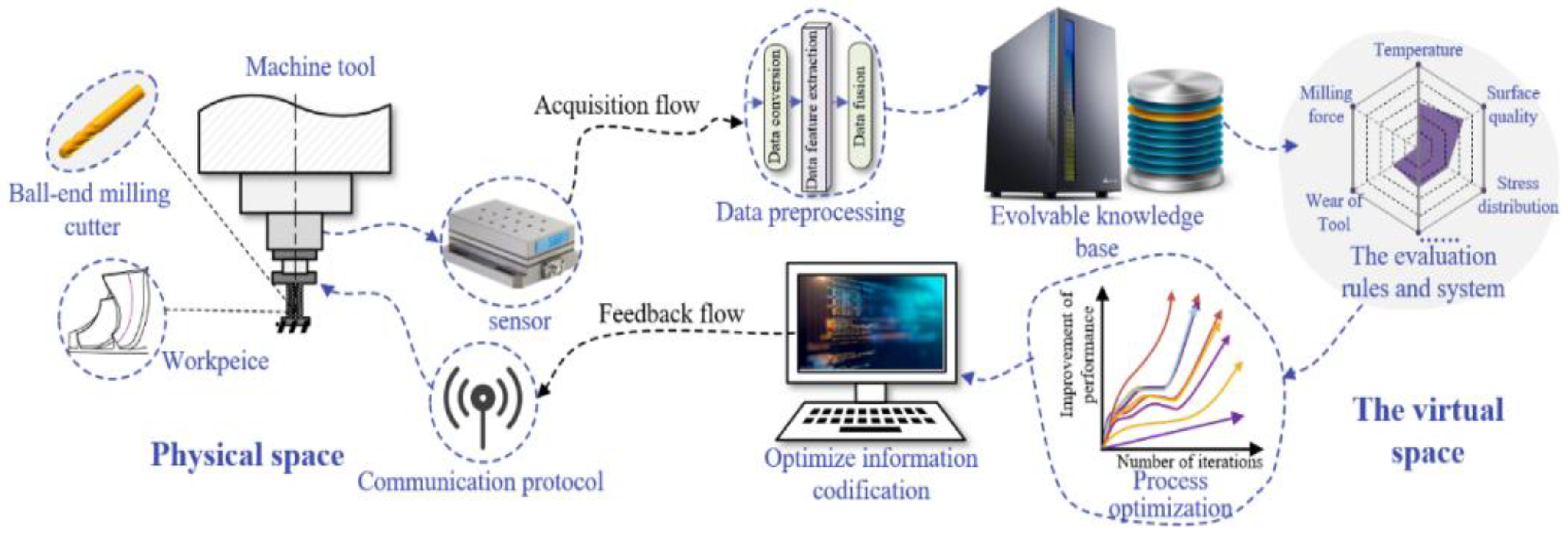
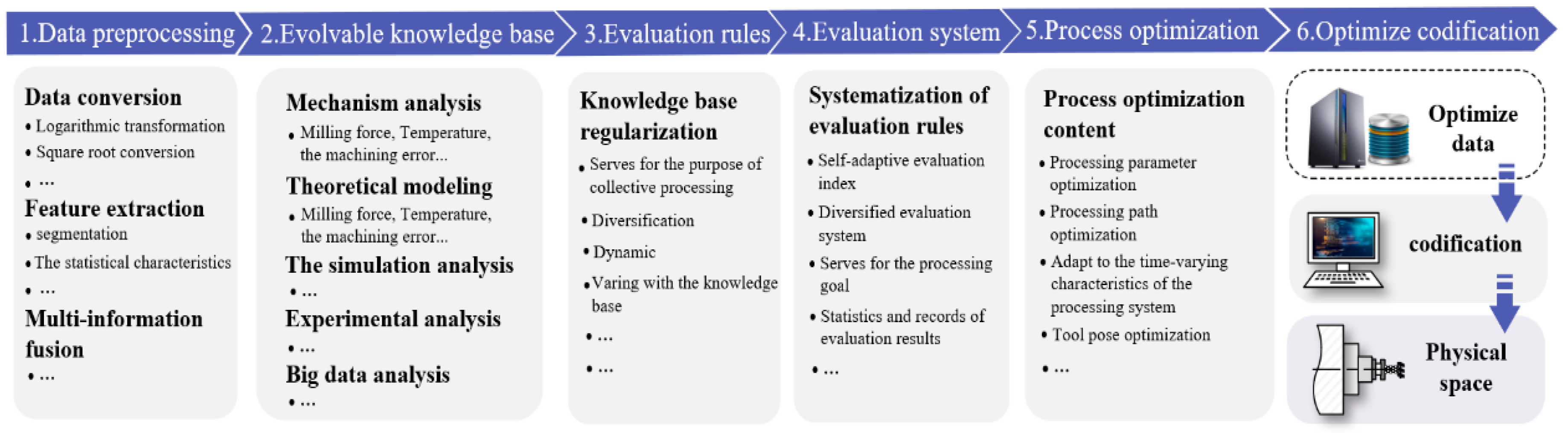
2. Digital–Twin Model Based on Specific Processing Technology
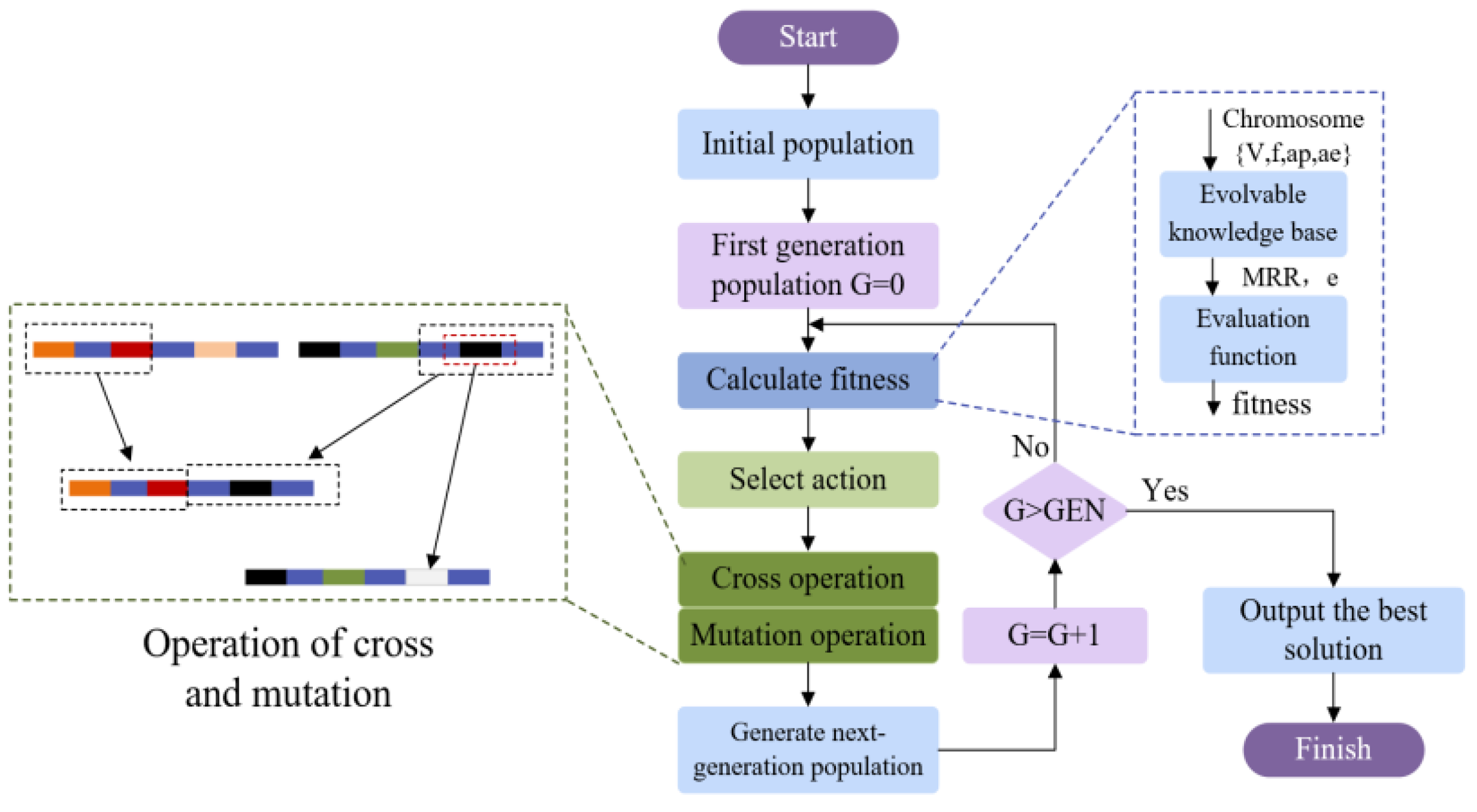
2.1. Digital–Twin Optimization Model Based on Specific Processing Technology
- (1)
- Data preprocessing module
- (2)
- Evolvable knowledge base module
- (3)
- Process evaluation rule module
- (4)
- The process evaluation system module
- (5)
- The process optimization module
- (6)
- Optimize the information digitization module
2.2. TC4 Impeller Blade Machining Digital–Twin Model
3. Digital–Twin Model Evolvable Knowledge Base Module
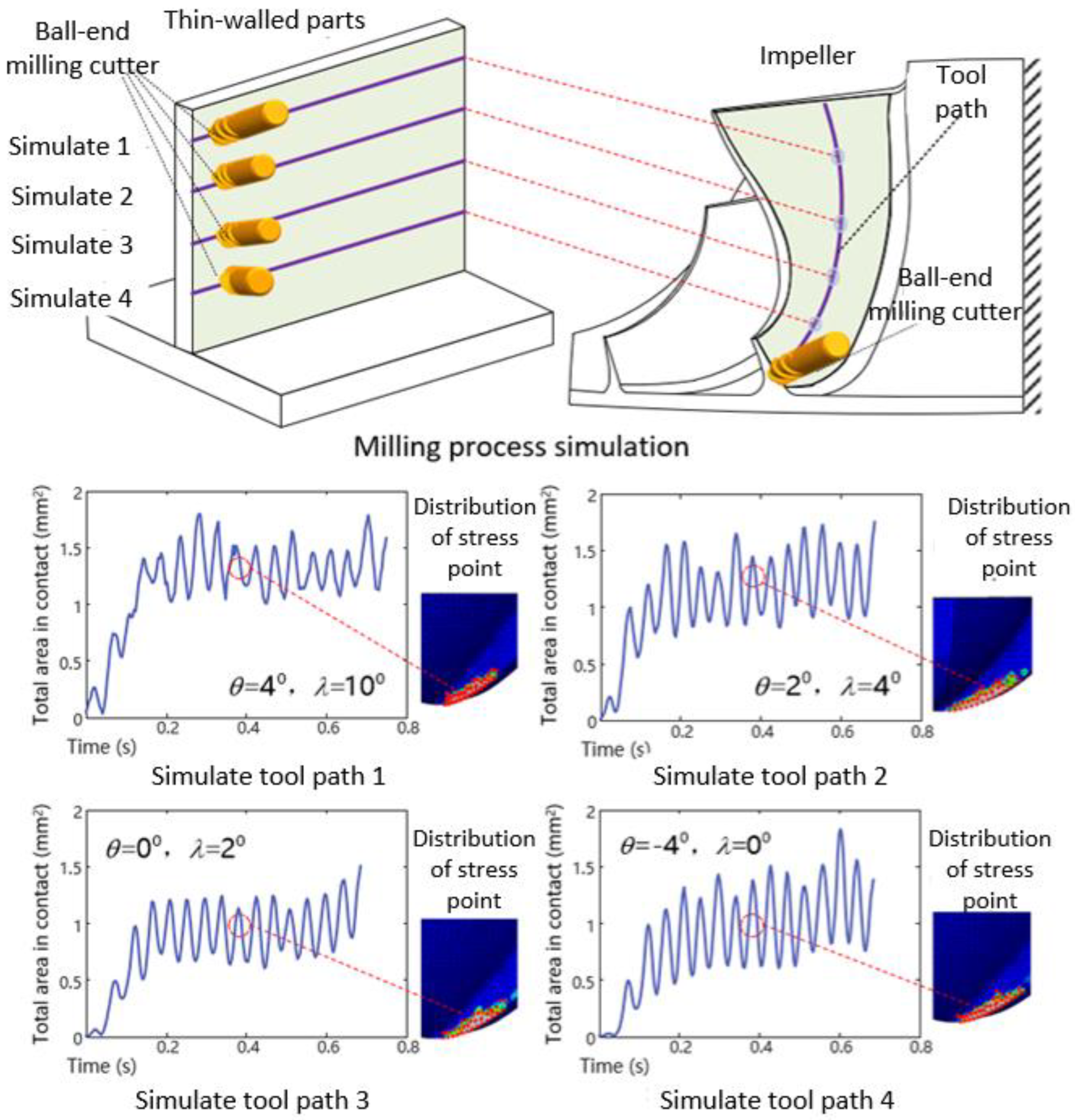
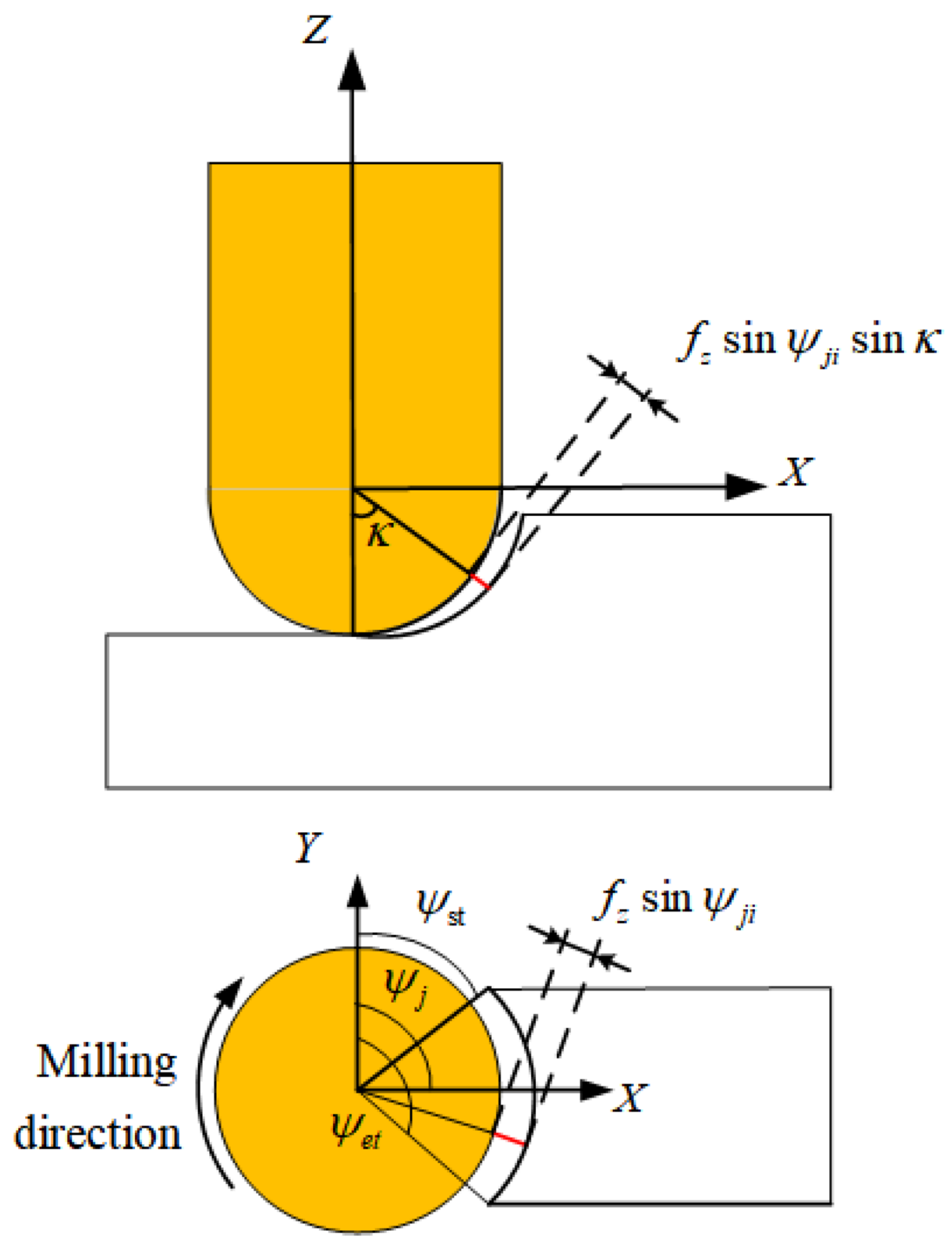
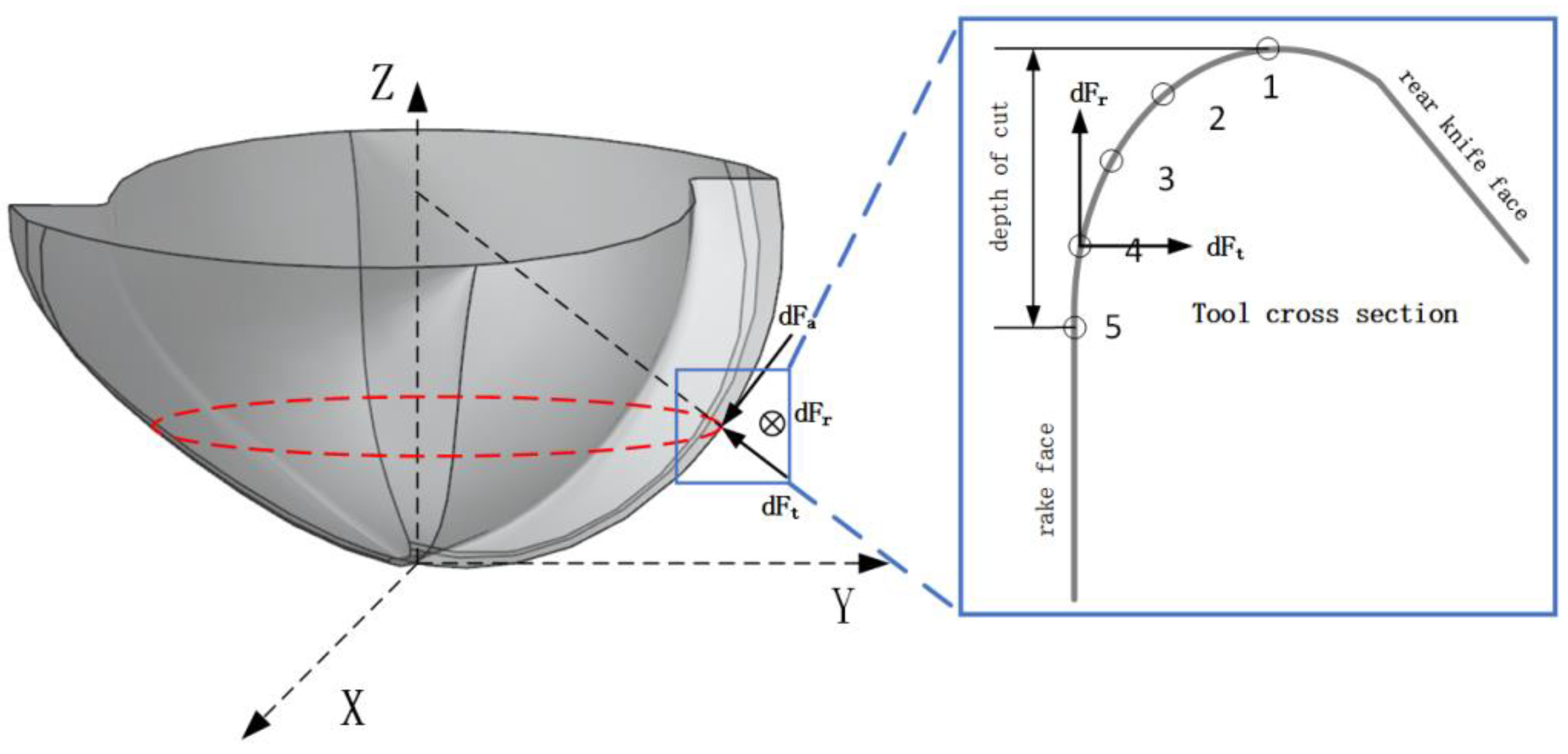
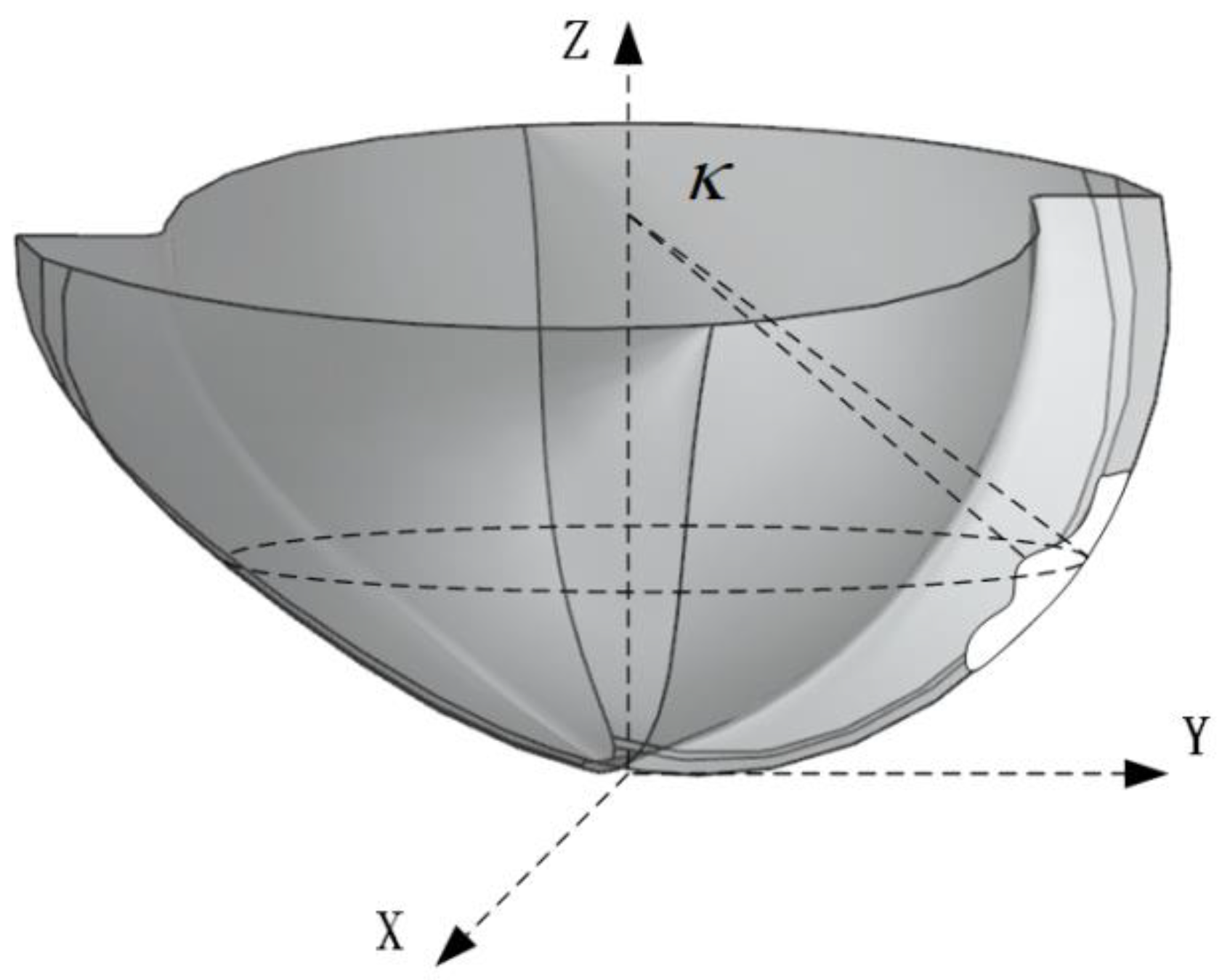
3.1. Solution of Tool–Workpiece Cutting Contact Relationship
3.2. Revised Model of Unreformed Cutting Thickness under Tool Wear Conditions
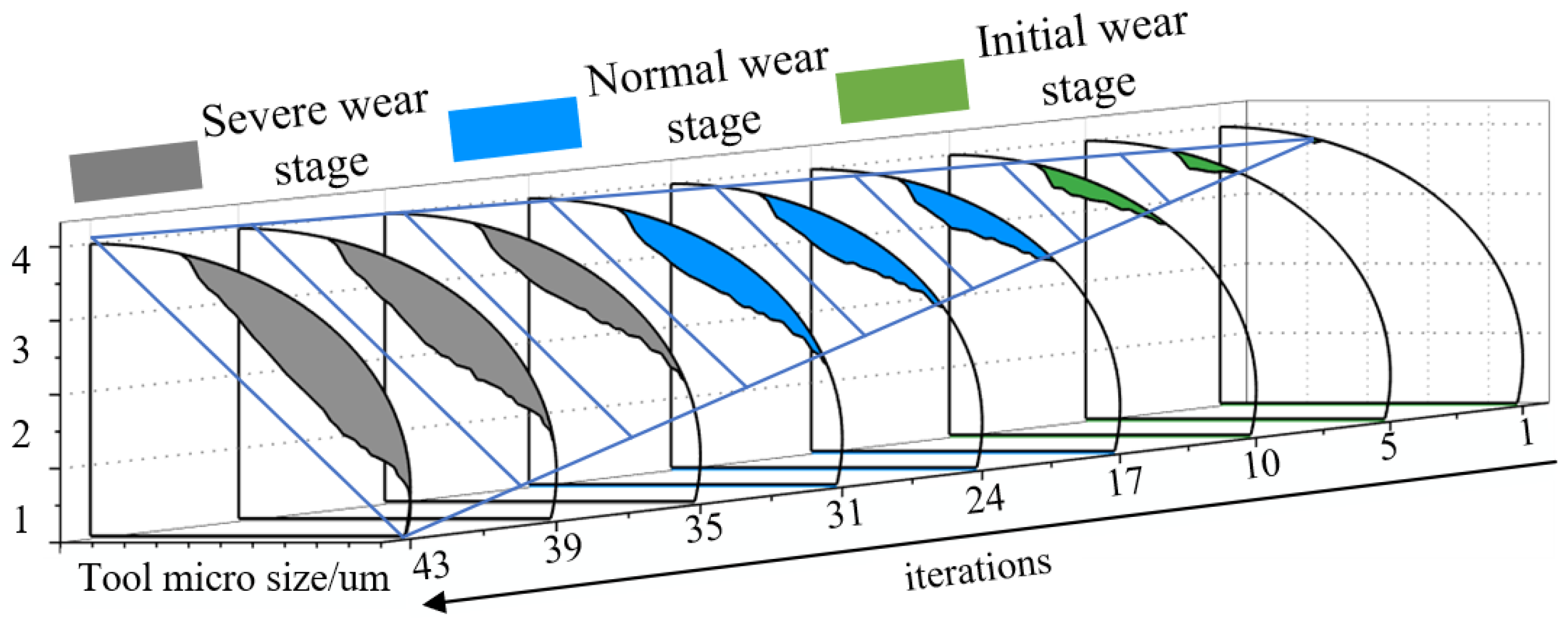
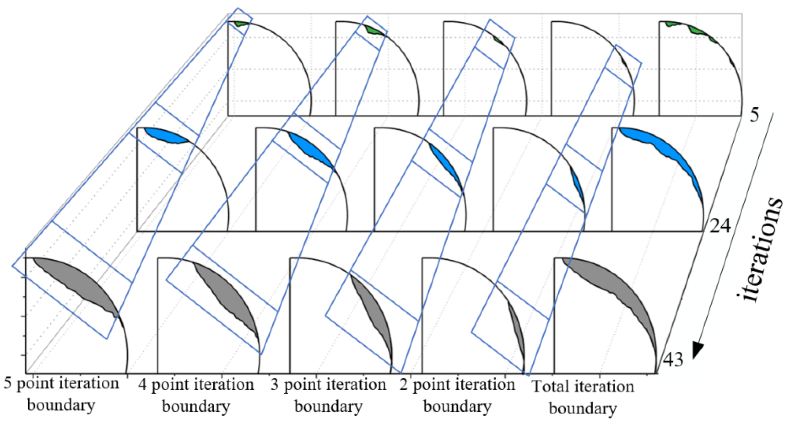
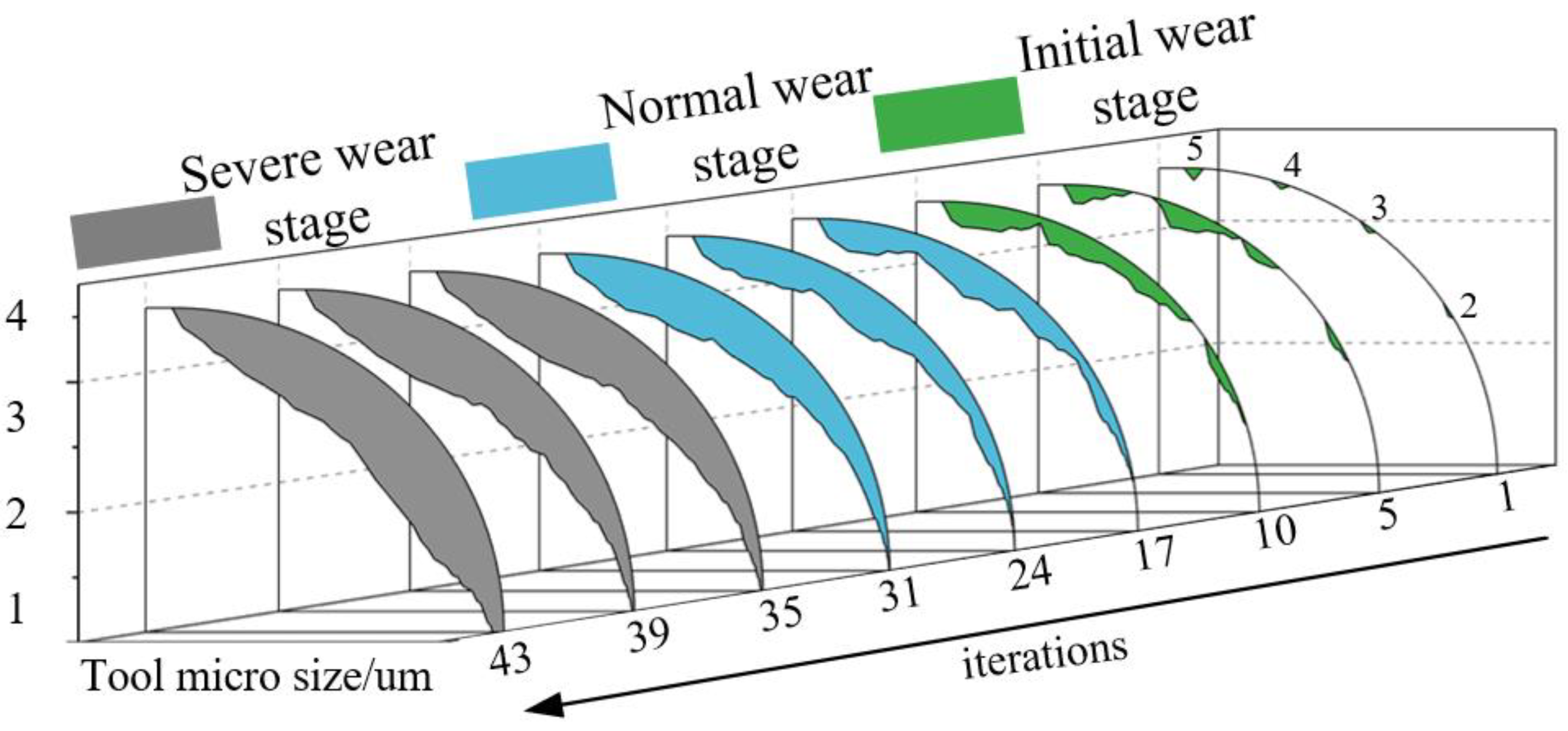
3.2.1. Construction of an Evolutionary Knowledge Base Model Based on Tool Wear Prediction Model
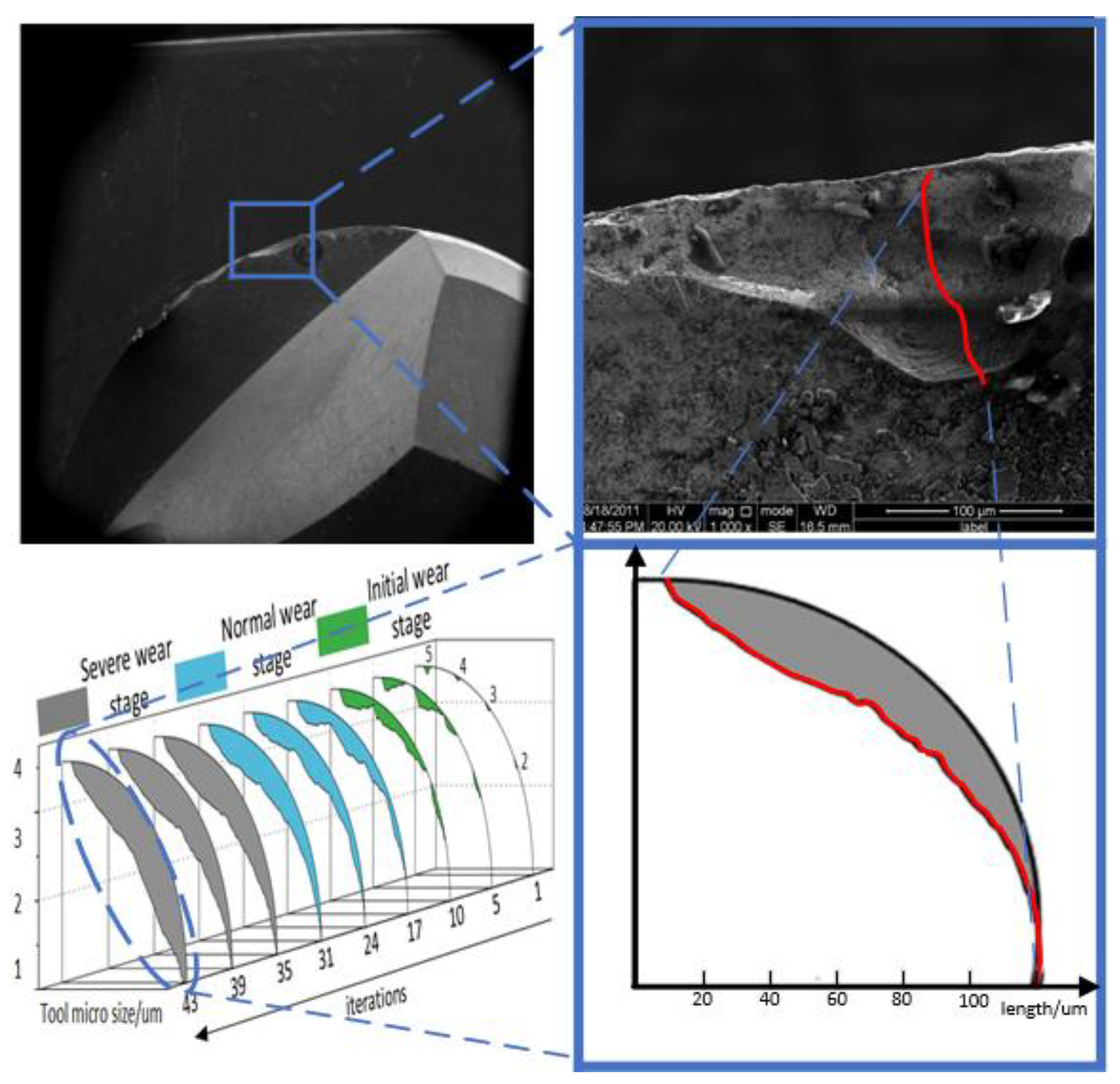
3.2.2. Analysis
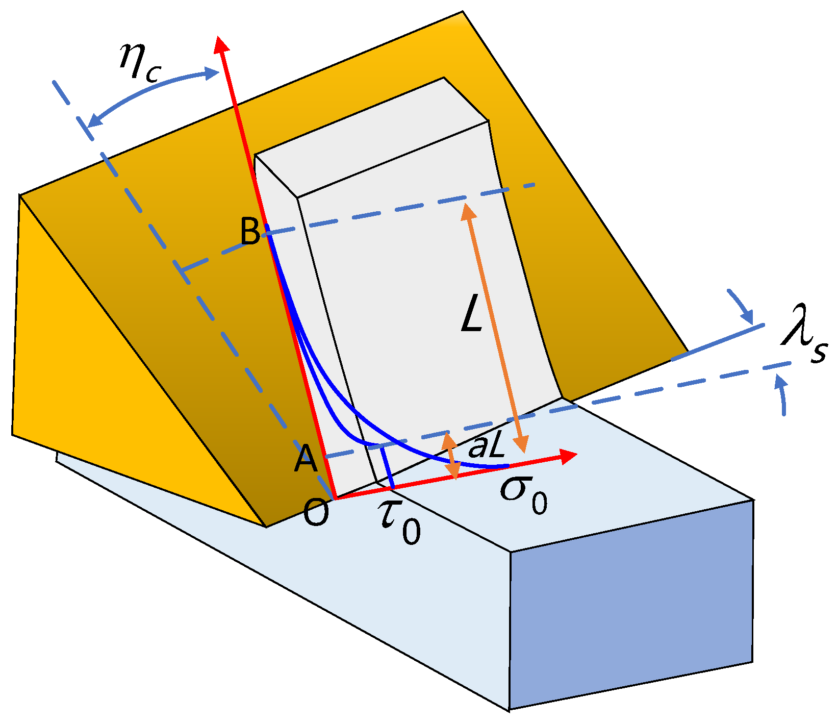
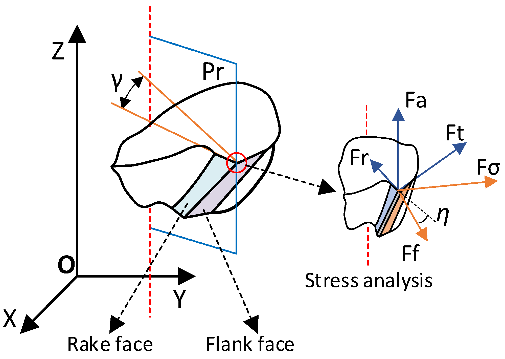
3.3. Milling Force Prediction Model Based on Tool–Chip Contact Relationship
4. Digital–Twin Model Optimization Module
4.1. Parameter Optimization Evaluation Rules
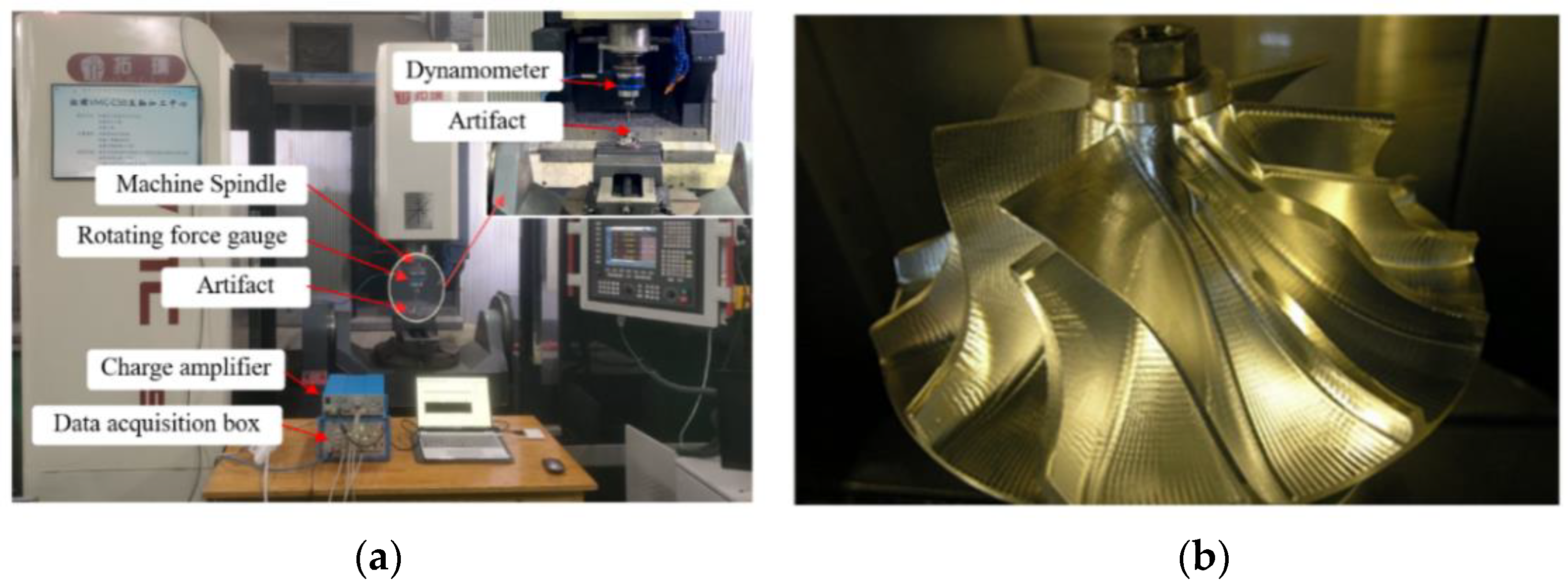
4.2. Digital–Twin Model Test Verification and Analysis
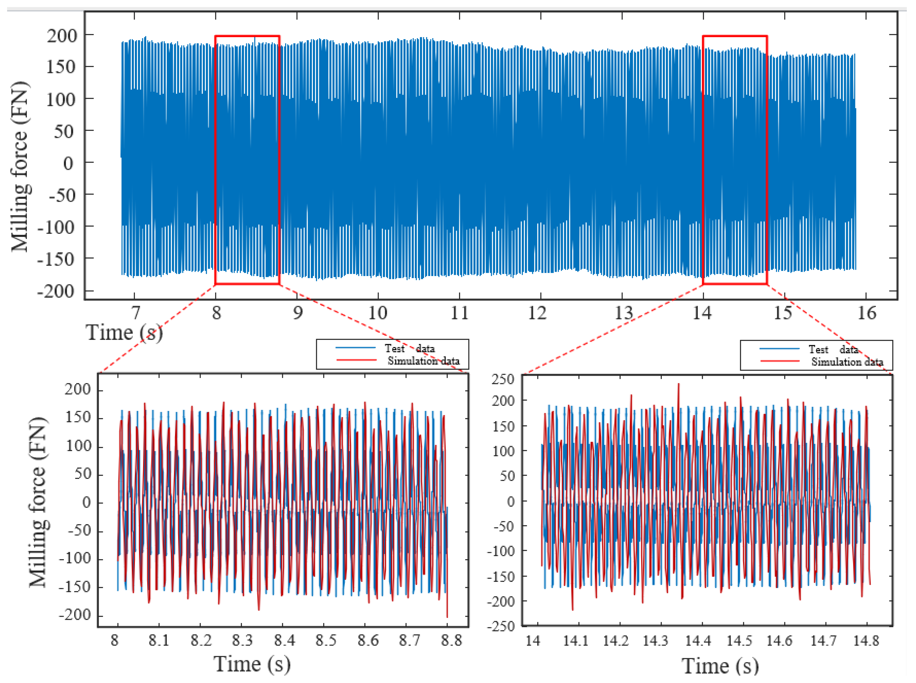
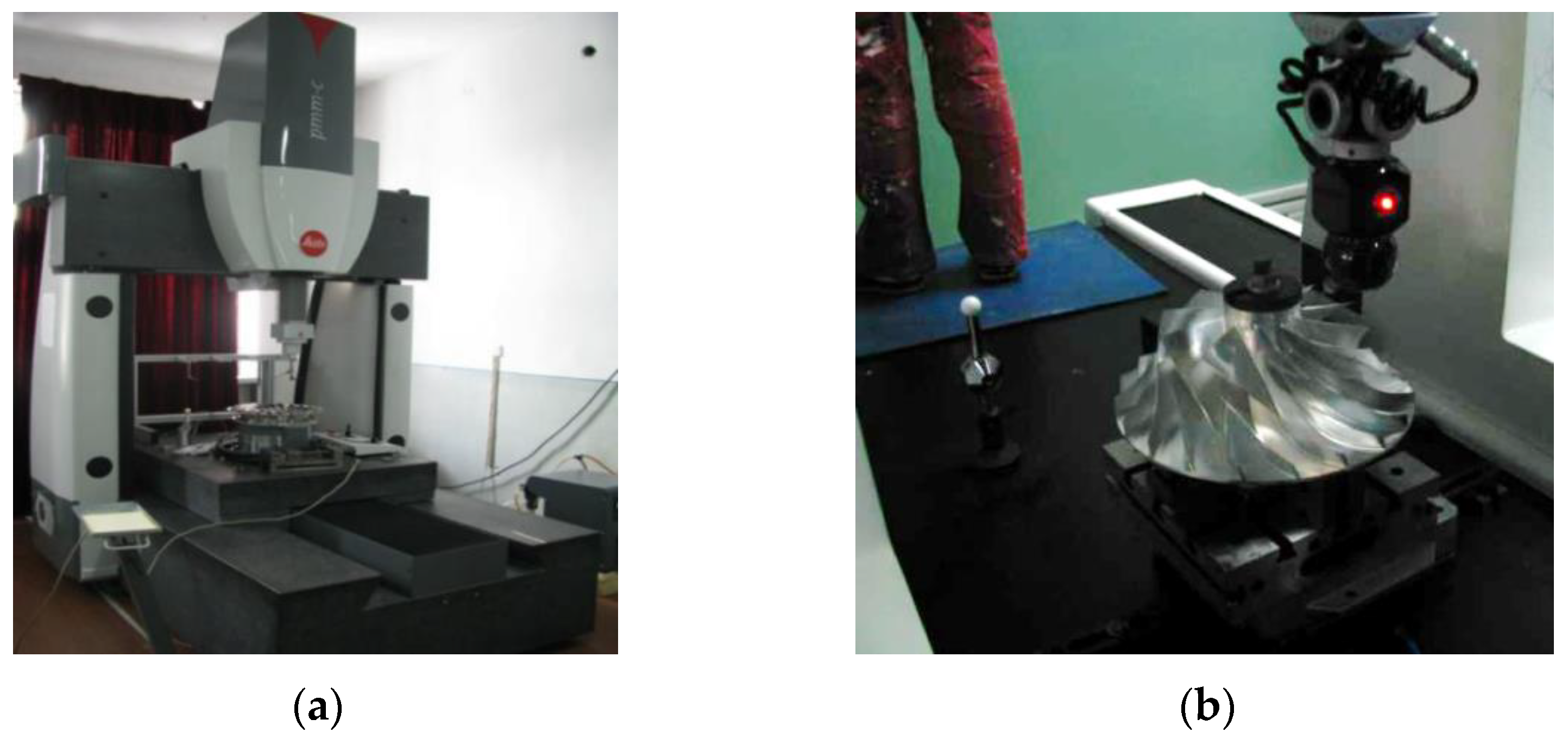
4.2.1. Digital–Twin Model Control Test
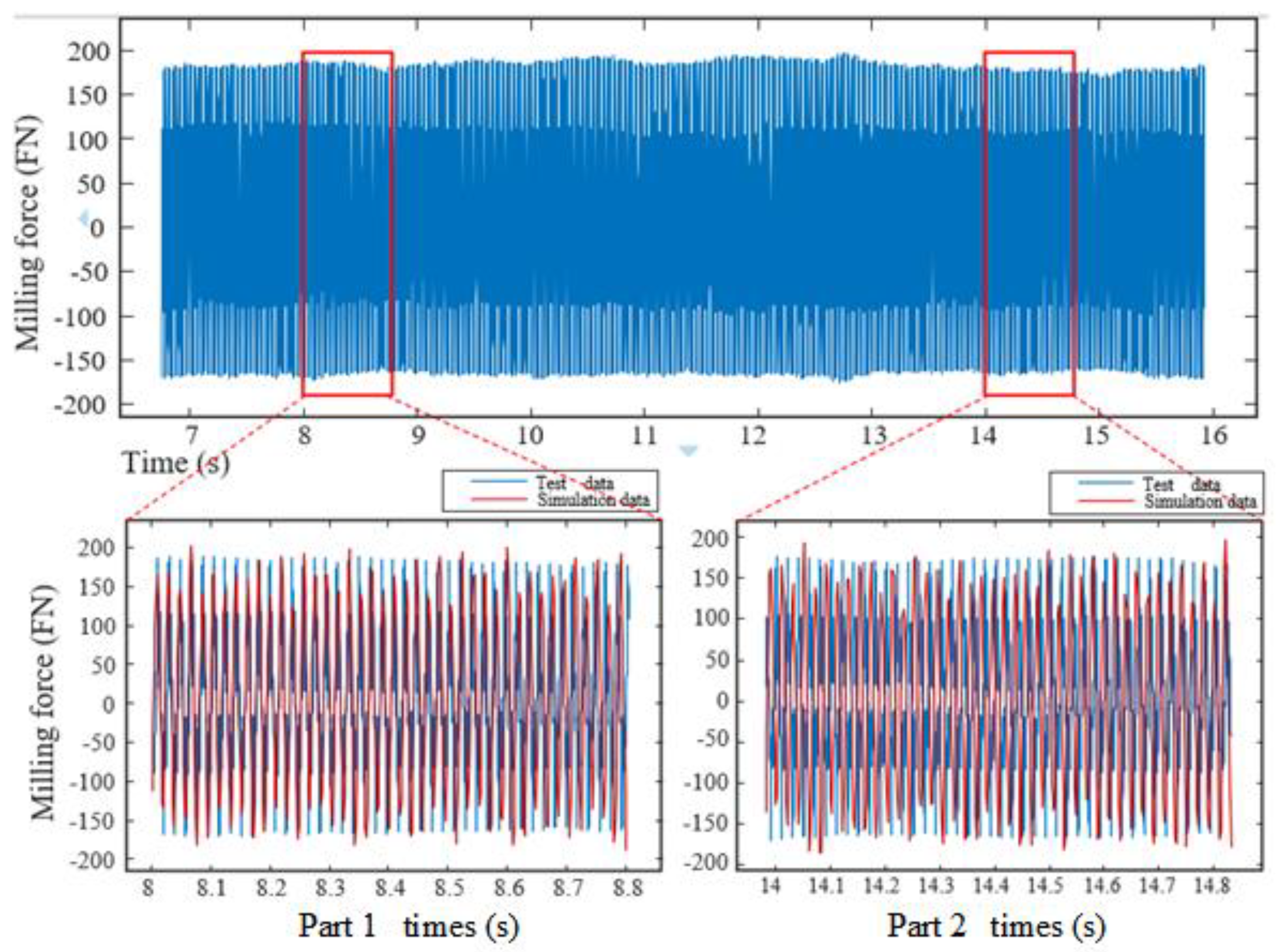
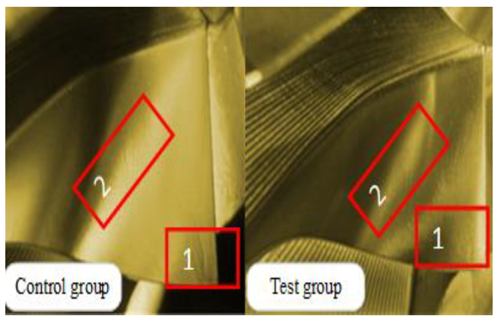
4.2.2. Experiments of the Digital–Twin Model Experimental Group
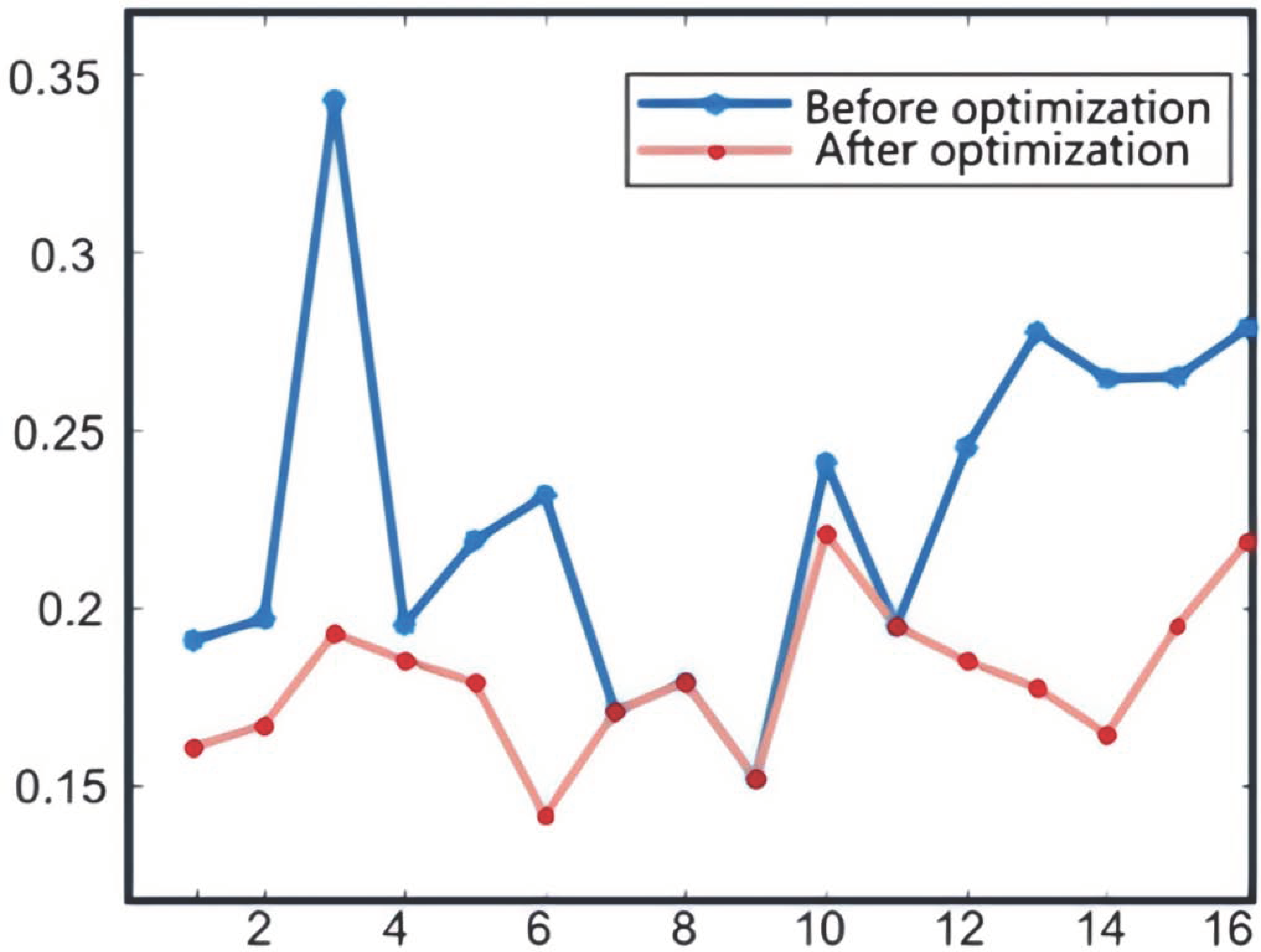
4.2.3. Discussion on Measurement Data of Impeller Blade Profile Error
5. Conclusions
- A digital–twin model based on the complex process of impeller blades was proposed. This model achieves the iterative feedback optimization of machining parameters for impeller blades. A TC4 digital–twin model has been established for specific machining process levels, achieving the data optimization of complex machining processes for impeller blades.
- Based on the digital–twin model, this article constructs an evolutionary knowledge base for impeller blade machining. Through secondary development, point cloud data are extracted from ABAQUS to construct a knowledge base, accurately expressing the contact relationship between tools and workpieces. At the same time, the tool wear model is established in the evolutionary knowledge base. The evolutionary knowledge base takes the spatial position information of the machine tool spindle and the angles of the turntable and swing table as real–time inputs. Based on rolling data and tool wear model, a milling force prediction model under the condition of tool wear was constructed. The prediction error of this model is less than 20%.
- Based on the coupling relationship between milling force and machining error, this article establishes an iterative model for milling force and machining error. This model achieves real–time feedback process control through data rolling and process iteration optimization based on machining quality evaluation. The digital–twin system calculates through an embedded model that the average time it takes to send out active control signals is less than 500 milliseconds. This improves the mapping accuracy of the digital–twin model.
Author Contributions
Funding
Institutional Review Board Statement
Informed Consent Statement
Data Availability Statement
Conflicts of Interest
References
- Rosen, R.; Von Wichert, G.; Lo, G.; Bettenhausen, K.D. About The Importance of Autonomy and digital–twins for the Future of Manufacturing. IFAC–Pap. 2015, 48, 567–572. [Google Scholar] [CrossRef]
- Grieves, M.W. Product Lifecycle Management: The New Paradigm for Enterprises. Int. J. Prod. Dev. 2005, 2, 71. [Google Scholar] [CrossRef]
- Fei, T.; Liu, W.; Liu, J.; Liu, X. Digital–twin and Its Potential Application Exploration. Comput. Integr. Manuf. Syst. 2018, 24, 1–18. [Google Scholar] [CrossRef]
- Fei, T.; Liu, W. Five–dimension digital–twin Model and Its Ten Applications. Jisuanji Jicheng Zhizao Xitong/Comput. Integr. Manuf. Syst. 2019, 25, 1–18. [Google Scholar]
- Liu, J.; Zhao, P.; Jing, X.; Cao, X.; Sheng, S.; Zhou, H.; Liu, X.; Feng, F. Dynamic design method of digital–twin process model driven by knowledge–evolution machining features. Int. J. Prod. Res. 2021, 60, 2312–2330. [Google Scholar] [CrossRef]
- Hänel, A.; Seidel, A.; Frieß, U.; Teicher, U.; Wiemer, H.; Wang, D.; Wenkler, E.; Penter, L.; Hellmich, A.; Ihlenfeldt, S. Digital–twins for High–Tech Machining Applications—A Model–Based Analytics–Ready Approach. J. Manuf. Mater. Process. 2021, 5, 80. [Google Scholar] [CrossRef]
- Bao, J.; Guo, D.; Li, J.; Zhang, J. The Modelling and Operations for The Digital–twin in the Context of Manufacturing. Enterp. Inf. Syst. 2019, 13, 534–556. [Google Scholar] [CrossRef]
- Delbrügger, T.; Rossmann, J. Representing Adaptation Options in Experimentable Digital–Twins of Production Systems. Int. J. Comput. Integr. Manuf. 2019, 32, 352–365. [Google Scholar] [CrossRef]
- Luo, W.; Hu, T.; Zhang, C.; Wei, Y. digital–twin for CNC machine tool: Modeling and using strategy. J. Ambient. Intell. Humaniz. Comput. 2019, 10, 1129–1140. [Google Scholar] [CrossRef]
- Xuemin, S.; Jinsong, B.; Jie, L.; Yiming, Z.; Shimin, L.; Bin, Z. A digital–twin–driven approach for the assembly–commissioning of high precision products. Robot. Comput. Integr. Manuf. 2020, 61, 101839. [Google Scholar]
- Hänel, A.; Schnellhardt, T.; Wenkler, E.; Nestler, A.; Brosius, A.; Corinth, C.; Fay, A.; Ihlenfeldt, S. The development of a digital–twin for machining processes for the application in aerospace industry. Procedia CIRP 2020, 93, 1399–1404. [Google Scholar] [CrossRef]
- Liu, S.; Bao, J.; Lu, Y.; Li, J.; Lu, S.; Sun, X. digital–twin modeling method based on biomimicry for machining aerospace components. J. Manuf. Syst. 2020, 58, 180–195. [Google Scholar] [CrossRef]
- Mukherjee, T.; Debroy, T. A digital–twin for rapid qualification of 3D printed metallic components. Appl. Mater. Today 2018, 14, 59–65. [Google Scholar] [CrossRef]
- Söderberg, R.; Wärmefjord, K.; Carlson, J.S.; Lindkvist, L. Toward a digital–twin for real–time geometry assurance in individualized production. CIRP Ann. Manuf. Technol. 2017, 66, 137–140. [Google Scholar] [CrossRef]
- Glatt, M.; Sinnwell, C.; Yi, L.; Donohoe, S.; Ravani, B.; Jan, C. Aurich. Modeling and Implementation of A Digital–Twin of Material Flows Based on Physics Simulation. J. Manuf. Syst. 2021, 15, 231–245. [Google Scholar] [CrossRef]
- Zhao, L.; Fang, Y.; Lou, P.; Yan, J. Cutting Parameter Optimization for Reducing Carbon Emissions Using digital–twin. Int. J. Precis. Eng. Manuf. 2021, 22, 933–949. [Google Scholar] [CrossRef]
- Ratchev, S.; Liu, S.; Becker, A.A. Error compensation strategy in milling flexible thin–wall parts. J. Mater. Process. Technol. 2005, 162, 673–681. [Google Scholar] [CrossRef]
- Chen, W.; Xue, J.; Tang, D.; Chen, H.; Qu, S. Deformation prediction and error compensation in multilayer milling processes for thin–walled parts. Int. J. Mach. Tools Manuf. 2009, 49, 859–864. [Google Scholar] [CrossRef]
- Wang, L.; Si, H. Machining deformation prediction of thin–walled workpieces in five–axis flank milling. Int. J. Adv. Manuf. Technol. 2018, 97, 4179–4193. [Google Scholar] [CrossRef]
- Liu, C.; Li, Y.; Shen, W. A real time machining error compensation method based on dynamic features for cutting force induced elastic deformation in flank milling. Mach. Sci. Technol. 2018, 22, 766–786. [Google Scholar] [CrossRef]
- Yue, C.; Chen, Z.; Liang, S.Y.; Gao, H. Modeling machining errors for thin–walled parts according to chip thickness. Int. J. Adv. Manuf. Technol. 2019, 10, 91–100. [Google Scholar] [CrossRef]
- Chen, Z.; Yue, C.; Liang, S.Y.; Liu, X.; Li, H. Iterative from error prediction for side–milling of thin–walled parts. Int. J. Adv. Manuf. Technol. 2020, 107, 4173–4189. [Google Scholar] [CrossRef]
- Archard, F. Contact and Rubbing of Flflat Surfaces. J. Appl. Phys. 1953, 24, 981–988. [Google Scholar] [CrossRef]
- Sun, Y.; Jiang, S. Predictive modeling of chatter stability considering force–induced deformation effect in milling thin–walled parts. Int. J. Mach. Tools Manuf. 2018, 135, 38–52. [Google Scholar] [CrossRef]
- Sun, Y.; Jia, J.; Xu, J.; Chen, M.; Niu, J. Path Feedrate and Trajectory Planning for Free–Form Surface Machining: A State-of-the-Art Review. Chin. J. Aeronaut. 2022, 35, 12–29. [Google Scholar] [CrossRef]
- Sun, Y.; Zheng, M.; Jiang, S.; Zhan, D.; Wang, R. A State-of-the-Art Review on Chatter Stability in Machining Thin–Walled Parts. Machines 2023, 11, 359. [Google Scholar] [CrossRef]
- Liu, X.; Li, R.; Wu, S.; Yang, L.; Yue, C. A prediction method of milling chatter stability for complex surface mold. Int. J. Adv. Manuf. Technol. 2017, 89, 2637–2648. [Google Scholar] [CrossRef]
- Pirso, J.; Letunovit, S.; Viljus, M. Friction and wear behaviour of cemented carbides. Wear 2004, 257, 257–265. [Google Scholar] [CrossRef]
- Lancaster, J.K. The influence of substrate hardness on the formation and endurance of molybdenum disulphide films. Wear 1965, 10, 103–117. [Google Scholar] [CrossRef]
- Ge, G.; Du, Z.; Yang, J. Rapid prediction and compensation method of cutting force–induced error for thin–walled workpiece. Int. J. Adv. Manuf. Technol. 2020, 106, 5453–5462. [Google Scholar] [CrossRef]
- Lee, P.; Altinta, Y. Prediction of ball–end milling forces from orthogonal cutting data. Int. J. Mach. Tools Manuf. 1996, 36, 1059–1072. [Google Scholar] [CrossRef]
- Gradisek, J.; Kalveram, M.; Weinert, K. Mechanistic identification of specific force coefficientsfor a general end mill. Int. J. Mach. Tools Manuf. 2004, 44, 401–414. [Google Scholar] [CrossRef]
- Budak, E.; Ozlu, E. Development of a thermomechanical cutting process model for machining process simulations. CIRP Ann. Manuf. Technol. 2008, 57, 97–100. [Google Scholar] [CrossRef]
- Özlü, E.; Budak, E.; Molinari, A. Thermomechanical modeling of orthogonal cutting including the effect of stick–slide regions on the rake face. In Proceedings of the 10th CIRP International Workshop on Modeling of Machining Operations, Reggio Calabria, Italy, 27–28 August 2007; University of Calabria: Arcavacata, Italy, 2007. [Google Scholar]


| Parameter | Numerical Value | Parameter | Numerical Value |
|---|---|---|---|
| Density (kg/m3) | 14,500 | Hardness/HA | 1154 |
| Elasticity modulus/GPa | 640 | Heatconductivity coefficient (W/m·K) | 75.4 |
| Yield strength/MPa | 2600 | Poisson’s ratio | 0.22 |
| Side rake angle/° | 4 | Helix angle/° | 30 |
| Number of cutting edges | 2 | Rake angle/° | 2 |
| Parameter | Numerical Value | Parameter | Numerical Values |
|---|---|---|---|
| Speed rad/min | 15,000 | The x–axis is the travel of the table/mm | 1050 |
| Spindle power/KW | 11 | The y–axis is the travel of the table/mm | 560 |
| Maximum feed speed 25 m/min | 2600 | The z–axis is the travel of the table/mm | 450 |
| Positioning accuracy/mm | 0.005 | The a–axis is the travel of the table/° | −25°/100° |
| Cooling method | Oil cooled | The c–axis is the travel of the table/° | N*360° |
| Parameter | Numerical Value | Parameter | Numerical Values |
|---|---|---|---|
| Speed rad/min | 15,000 | The x–axis is the travel of the table | 1050 mm |
| Spindle power(KW) | 11 | The y–axis is the travel of the table | 560 |
| Maximum feed speed 25 m/min | 2600 | The z–axis is the travel of the table | 450 |
| Positioning accuracy is 0.005 mm | 4° | The a–axis is the travel of the table | −25°/100° |
| Cooling method | Oil cooled | The c–axis is the travel of the table | N*360° |
| Data/Prediction Error | Peak Error | Amplitude Error | Maximum Peak Error | Maximum Amplitude Error |
|---|---|---|---|---|
| Control group 1 | 7.34% | 5.57% | 13.21% | 14.69% |
| Test group 1 | 7.39% | 5.59% | 11.5% | 11.48% |
| Control group 2 | 8.21% | 6.65% | 18.62% | 18.32% |
| Test group 2 | 7.9% | 6.75% | 12.5% | 13.77% |
| Name | Deviation | Refer–X | Refer–Y | Refer–Z | Measure–X | Measure–Y | Measure–Z |
|---|---|---|---|---|---|---|---|
| C001 | 0.1908 | −35.4959 | −70.5772 | 13.6864 | −35.9428 | −70.7604 | 13.6535 |
| C002 | 0.1969 | −35.7894 | −70.8760 | 16.0371 | −35.1890 | −70.0496 | 16.0055 |
| C003 | 0.3427 | −36.0747 | −60.2227 | 19.1029 | −36.4087 | −60.2957 | 19.0782 |
| C004 | 0.1952 | −36.5743 | −58.5549 | 20.3823 | −36.7770 | −58.5856 | 20.3726 |
| C005 | 0.2189 | −38.2148 | −55.5444 | 22.1072 | −38.4213 | −58.5526 | 22.0261 |
| C006 | 0.2315 | −38.7591 | −52.4318 | 24.9614 | −38.9826 | −52.4152 | 24.9032 |
| C007 | 0.1708 | −42.3633 | −48.6112 | 26.6700 | −43.0371 | −48.5946 | 26.5191 |
| C008 | 0.1791 | −43.8166 | −44.9163 | 29.2822 | −43.0138 | −29.8878 | 29.1482 |
| C009 | 0.1518 | −43.3029 | −43.4705 | 33.5623 | −43.5723 | −43.4053 | 33.4193 |
| C010 | 0.2407 | −43.0976 | −42.1685 | 36.0519 | −42.9160 | −42.1691 | 36.2098 |
| C011 | 0.1947 | −42.5740 | −46.7001 | 37.0076 | −42.3747 | −47.0267 | 37.1289 |
| C012 | 0.2450 | −42.5818 | −47.1489 | 39.1056 | −41.9664 | −47.1790 | 38.9184 |
| C013 | 0.2774 | −37.1423 | −47.9029 | 40.5872 | −37.8828 | −49.1982 | 39.6851 |
| C014 | 0.2644 | −37.6970 | −49.6733 | 41.5810 | −37.4448 | −50.1837 | 40.4595 |
| C015 | 0.1751 | −36.7832 | −59.4247 | 43.3747 | −36.8333 | −59.4769 | 43.2344 |
| C016 | 0.2649 | −35.0406 | −58.1229 | 42.6113 | −36.7836 | −58.0864 | 43.6643 |
| Name | Deviation | Refer–X | Refer–Y | Refer–Z | Measure–X | Measure–Y | Measure–Z |
|---|---|---|---|---|---|---|---|
| C001 | 0.1608 | −35.3359 | −70.5001 | 13.1862 | −35.8664 | −71.2604 | 14.0235 |
| C002 | 0.1669 | −35.1653 | −70.1356 | 16.0355 | −35.2210 | −70.0096 | 15.8051 |
| C003 | 0.1927 | −37.3454 | −61.2227 | 19.2588 | −37.4022 | −61.0021 | 19.556 |
| C004 | 0.1852 | −36.1733 | −58.1519 | 19.8823 | −36.5710 | −58.2853 | 19.0211 |
| C005 | 0.1789 | −39.2036 | −54.3177 | 21.9072 | −39.5656 | −54.4426 | 21.8856 |
| C006 | 0.1415 | −41.5497 | −51.9996 | 24.3301 | −41.8897 | −51.7325 | 24.8688 |
| C007 | 0.1708 | −43.4464 | −49.5998 | 27.3200 | −43.0358 | −48.9940 | 27.5111 |
| C008 | 0.1791 | −44.0243 | −49.7780 | 30.1663 | −44.0212 | −49.8848 | 30.1168 |
| C009 | 0.1518 | −45.0251 | −43.8805 | 34.4544 | −45.4432 | −44.0021 | 34.0023 |
| C010 | 0.2207 | −46.0877 | −42.1511 | 35.8522 | −42.889 | −43.0501 | 36.1231 |
| C011 | 0.1947 | −44.4610 | −47.1134 | 38.0016 | −42.5445 | −47.5017 | 37.5551 |
| C012 | 0.1850 | −43.1838 | −48.0211 | 38.7056 | −41.7711 | −48.1121 | 38.3211 |
| C013 | 0.1774 | −38.0198 | −47.8990 | 40.5587 | −38.9886 | −49.9969 | 39.5616 |
| C014 | 0.1644 | −38.9989 | −48.0532 | 41.0023 | −38.0112 | −50.6689 | 40.5588 |
| C015 | 0.1842 | −37.7842 | −47.1042 | 41.1024 | −37.7632 | −48.5631 | 40.9451 |
| C016 | 0.1949 | −36.0902 | −59.4229 | 43.3356 | −36.8898 | −59.0565 | 43.7441 |
Disclaimer/Publisher’s Note: The statements, opinions and data contained in all publications are solely those of the individual author(s) and contributor(s) and not of MDPI and/or the editor(s). MDPI and/or the editor(s) disclaim responsibility for any injury to people or property resulting from any ideas, methods, instructions or products referred to in the content. |
© 2023 by the authors. Licensee MDPI, Basel, Switzerland. This article is an open access article distributed under the terms and conditions of the Creative Commons Attribution (CC BY) license (https://creativecommons.org/licenses/by/4.0/).
Share and Cite
Li, R.; Wang, S.; Wang, C.; Wang, S.; Zhou, B.; Liu, X.; Zhao, X. Research into Dynamic Error Optimization Method of Impeller Blade Machining Based on Digital–Twin Technology. Machines 2023, 11, 697. https://doi.org/10.3390/machines11070697
Li R, Wang S, Wang C, Wang S, Zhou B, Liu X, Zhao X. Research into Dynamic Error Optimization Method of Impeller Blade Machining Based on Digital–Twin Technology. Machines. 2023; 11(7):697. https://doi.org/10.3390/machines11070697
Chicago/Turabian StyleLi, Rongyi, Shanchao Wang, Chao Wang, Shanshan Wang, Bo Zhou, Xianli Liu, and Xudong Zhao. 2023. "Research into Dynamic Error Optimization Method of Impeller Blade Machining Based on Digital–Twin Technology" Machines 11, no. 7: 697. https://doi.org/10.3390/machines11070697
APA StyleLi, R., Wang, S., Wang, C., Wang, S., Zhou, B., Liu, X., & Zhao, X. (2023). Research into Dynamic Error Optimization Method of Impeller Blade Machining Based on Digital–Twin Technology. Machines, 11(7), 697. https://doi.org/10.3390/machines11070697