Article

Transfer Learning Based Fault Detection for Suspension System Using Vibrational Analysis and Radar Plots

by
Samavedam Aditya Sai
1,
Sridharan Naveen Venkatesh
1,
Seshathiri Dhanasekaran
2,*,
Parameshwaran Arun Balaji
1,
Vaithiyanathan Sugumaran
1,
Natrayan Lakshmaiya
3 and
Prabhu Paramasivam
4
1
School of Mechanical Engineering, Vellore Institute of Technology, Vandalur—Kelambakkam Road, Keelakottatiyur, Chennai 600127, India
2
Department of Computer Science, UiT The Arctic University of Norway, 9037 Tromsø, Norway
3
Department of Mechanical Engineering, Saveetha School of Engineering, SIMATS, Chennai 602105, India
4
Department of Mechanical Engineering, College of Engineering and Technology, Mettu University, Mettu 318, Ethiopia
*
Author to whom correspondence should be addressed.
Machines 2023, 11(8), 778; https://doi.org/10.3390/machines11080778
Submission received: 28 June 2023 / Revised: 17 July 2023 / Accepted: 24 July 2023 / Published: 26 July 2023
(This article belongs to the Special Issue Data-Driven Fault Diagnosis for Machines and Systems)

Abstract

:
The suspension system is of paramount importance in any automobile. Thanks to the suspension system, every journey benefits from pleasant rides, stable driving and precise handling. However, the suspension system is prone to faults that can significantly impact the driving quality of the vehicle. This makes it essential to find and diagnose any faults in the suspension system and rectify them immediately. Numerous techniques have been used to identify and diagnose suspension faults, each with drawbacks. This paper’s proposed suspension fault detection system aims to detect these faults using deep transfer learning techniques instead of the time-consuming and expensive conventional methods. This paper used pre-trained networks such as Alex Net, ResNet-50, Google Net and VGG16 to identify the faults using radar plots of the vibration signals generated by the suspension system in eight cases. The vibration data were acquired using an accelerometer and data acquisition system placed on a test rig for eight different test conditions (seven faulty, one good). The deep learning model with the highest accuracy in identifying and detecting faults among the four models was chosen and adopted to find defects. The results state that VGG16 produced the highest classification accuracy of 96.70%.

1. Introduction

Cars account for most vehicles on the roads nowadays, with the tally increasing daily. Nowadays, cars are expected to have top-notch performance and handling characteristics due to rapid advancements in the automotive field. Furthermore, the provision for enhanced comfort is considered the manufacturer’s responsibility to be implemented without compromising reliability. Driver and passenger comfort rely heavily on the suspension system due to its shock-absorbing feature. Suspension dampens any force inflicted on the tires and the vehicle due to road irregularities and ensures that the vehicle stays unharmed. Despite this, the major function of the suspension system is to manage the vehicle’s handling characteristics by maximizing the friction between the tires and the road and ensuring that the vehicle can be steered easily and quickly with a high degree of stability. However, regular use of the vehicle results in vehicle parts’ wear and tear, and the suspension system is not immune to this. Hence, the suspension system must be designed so that these types of failures do not impact the performance characteristics of the system. Recent advancements in suspension system technologies have found a way to improve the reliability and performance of the suspension system as a whole [1]. However, such systems come at a high cost due to the system’s complexity. This is reason enough for most manufacturers of vehicles to stick with the standard and low-cost alternatives that are unreliable and wear resistant. The suspension system contains many essential components that must work in tandem to achieve perfection. Among the integral parts, the ball joints and strut are prone to wear and tear due to fluctuating loads under varying conditions for a prolonged period of operation. These faults must be identified and rectified at the earliest so that the damage does not fester and cause other components to fail. Failed components can end up causing a lot of harm, making the vehicle highly unsafe for road travel. An exemplary fault diagnosis system would alert the vehicle driver, who would act upon it and nip the issue in the bud [2]. Fault diagnosis can be achieved in numerous ways. The currently available suspension fault detection systems use mathematical and machine learning models.
The most common mathematical and machine learning models researchers use for the fault detection [3] of suspension systems are presented in Table 1 as follows.
Field of suspension system fault detection has gained vast amounts of traction over the past few years. Zhu et al. examined the use of mathematical models to construct three fault detection filters for three different finite frequency domains [14]. Similarly, Azadi & Soltani proposed a wavelet transform method to detect faults in suspension systems [15]. In 2002 Börner et al. proposed a fault detection system with parameter estimation and the parity equations method using a microcontroller [16]. While these studies have demonstrated the effectiveness of mathematical and machine learning models, there are also certain limitations. Mathematical models have proven highly complicated and sensitive to model parameters. Similarly, the demanding selection and feature extraction processes contribute to the complexity of building effective machine-learning models. These steps, although distinct, add intricacy to the model development process, especially as the complexity of features increases. On the other hand, deep learning models and networks learn without performing feature extraction. Deep learning models work by creating complex neural networks capable of learning and identifying patterns over large numbers of data. These networks consist of layers of interconnected nodes, each performing a specific computation on the input it receives. The resulting output produced by each layer acts as the feed for the upcoming layer, gradually enabling the network to learn more complex representations and features of the data. Throughout the training process, the model adjusts the connection weights between all nodes to minimize the dissimilarity between the predicted feed and the proper feed of the data. This process is repeated many times with different data samples, allowing the model to learn all the intricacies of the patterns and the relationships between the input and output. Once the model is trained, predictions on new and unseen data can be performed with a significant level of precision in a relatively low time which depends on the exact model chosen. The use of deep learning models in fault diagnosis is a relatively new concept and has been in the incubation period for a considerable time (Figure 1). Only a few researchers have found use for deep learning models for fault detection. Liu & Gryllias discussed using ML and DL models to detect faults in rolling element bearings [17]. Vasan et al. discussed another application of DL and harnessed its power to monitor tire pressure and detect punctures in vehicles [18]. Similarly, faults in automobile dry clutches were diagnosed and detected by Chakrapani & Sugumaran with the help of a transfer learning-based DL model [19]. Some more studies on applying DL models in machines are presented in Table 2.
The fault detection and diagnosis of rotating machines such as the gearbox and roller bearings were performed by Tang et al. in 2020 with intelligent DL models [20]. DL models for fault detection do not end here; deep learning models along with SVM were used for fault detection in automobile hydraulic brake systems by Jegadeeshwaran & Sugumaran in 2015 [21]. Railway bogies bearing faults were diagnosed by Ding et al., with the ultimate power of lightweight multiscale convolutional neural networks (CNNs) [22]. Deep learning models have also found use in fault detection in concrete in the past few years by Tanyildizi et al. The authors devised a method to gauge the properties of concrete containing silica fumes exposed to extremely high temperatures using DL models [23]. Similarly, Ai et al. used convolutional neural networks to identify substantial structural damage [24]. Deep learning models have recently also found use in the medical industry. Fraz et al. suggested using DL models to perform multiscale segmentation on the exudates present in retinal images using context clues with the assistance of ensemble classification [25]. Mo et al. explored the application of cascaded deep residual networks for detecting diabetic macular edema in retinal images [26]. Deep learning models have also found use in detecting epileptic and neonatal seizures, as discussed by AH et al. and Nogay & Adeli [27,28]. Welding defect detection was also performed by Y. Zhang et al. and Z. Zhang et al. [29,30]. CNNs have become the preferred method in different domains. They have found use and are being widely used for fault diagnosis, image and video segmentation, object recognition and medical diagnosis tasks in contemporary applications due to their ability to automatically learn hierarchical features from raw input data, their scalability to handle large datasets and complex tasks and their superior performance compared to conventional machine learning approaches in various computer vision and image processing tasks. Additionally, CNNs offer translation invariance, regularization techniques, spatial and temporal learning capabilities and the ability to leverage transfer learning, making them an effective tool for various applications in various domains.
Table 2. Other implementations of deep learning in fault detection in mechanical systems.
ReferenceDeep Learning Techniques UsedMechanical System
[31]Optimized deep belief networkRolling Bearing
[32]Deep convolution neural network
[33]Ensemble learning method
[34]Stacked auto encoderGearbox
[35]Transfer learningSpark ignition engine
[36]Stacked denoising auto encoderCentrifugal Pumps
[37]Deep belief networkInduction Motor
[38]Artificial neural networksWind Turbines
The proposed method in this paper consists of three stages: data acquisition and collection, signal processing with image generation and decision making (classification). The first stage involves collecting data from accelerometers for every condition to obtain the required signals for fault diagnosis. In the second stage, the collected data are conditioned and transformed into a helpful form, i.e., radar plots that various deep learning models can analyze. In the final stage, a deep transfer learning model classifies the transformed signals (radar plots) and decides based on the classification results. Deep learning models have gained significant traction in fault diagnosis due to them having the power to classify images with high accuracy rates while overcoming some of the limitations of traditional machine learning models. Despite their potential, deep learning models require significant computational power to train and run. However, recent advancements have made deep learning more accessible to researchers and practitioners. Transfer learning is an emerging technique (based on deep learning) that enables the usage of pre-trained learned weights with particular domain knowledge to be transferred and applied in a different domain. Transfer learning can be effective in scenarios with a low volume of data, a lack of sufficient domain knowledge, minimal computational resources and complexity in building models from scratch. In the present study, transfer learning has been leveraged to classify radar plot pictures of eight different suspension conditions including one good and seven faulty cases. The seven faulty cases included tie rod ball joint worn off (TRBJ), strut worn off (STWO), lower arm bush worn off (LABW), low pressure in the wheel (LWP), strut external damage (STED), lower arm ball joint worn off (LABJ) and strut mount fault (STMF). Four popular deep learning networks were used in this study, namely VGG16, ResNet-50, AlexNet and GoogLeNet, to classify the images generated from the second stage of the proposed method. It is worth emphasizing that the accuracy achieved by DL models such as VGG16, ResNet-50, AlexNet and GoogLeNet can be significantly affected by various parameters which are referred to as “hyperparameters” which include batch size, epoch, solver and training test split ratio. The term “batch size” refers to the number of samples used in each training process. The epoch refers to the repeated usage of a specific quantity of the dataset to train the model. Finally, the split ratio determines the proportion of the dataset used for training and testing the model. Optimizing these hyperparameters is challenging and time-consuming, and their optimal values vary depending on the dataset and the model architecture. However, it is of the utmost importance to carefully tune these hyperparameters to ensure that the best possible classification accuracy of the deep learning models is achieved.
Technical contributions of the study
  • The overall experimental process carried out in the experimental study is presented in Figure 2. Vibration signals acquired using a piezoelectric accelerometer were converted into radar plots and pre-processed to be compatible with transfer learning networks considered in the study.
  • Post processing of the radar plots, pre-trained network performance was assessed for variations in hyperparameters such as solver, mini-batch-size, train-to-test ratio and initial learning rate.
  • The best performing network with optimal hyperparameters accurately classifying eight suspension conditions was determined.
  • The results obtained were then compared with various cutting-edge techniques to portray the superiority of the proposed methodology.
Novelty of the study
  • The paper introduces a novel experimental method using radar plots to visualize vibration data, offering a simpler alternative to complex techniques such as FFT, Hilbert Huang transform and empirical mode decomposition.
  • The study utilizes transfer learning with four pre-trained networks (VGG16, ResNet-50, AlexNet, and GoogLeNet) to classify radar plots representing eight suspension conditions.
  • The radar plots are used to classify various suspension cases, including worn tie rod ball joint (TRBJ), strut wear (STWO), lower arm bush wear (LABW), low pressure in the wheel (LWP), strut external damage (STED), worn lower arm ball joint (LABJ) and strut mount faults (STMF).
  • Hyperparameter variations were explored to optimize the performance of the pre-trained networks within the same dataset, resulting in the highest achievable classification accuracy for each network.
  • The proposed approach enables the generation of reliable radar plots for accurate analysis of suspension system faults.

2. Features of the Experimental System

This section will deal with the setup features, the method for data acquisition and the procedure for fault detection in suspension systems.

2.1. Experimental Setup

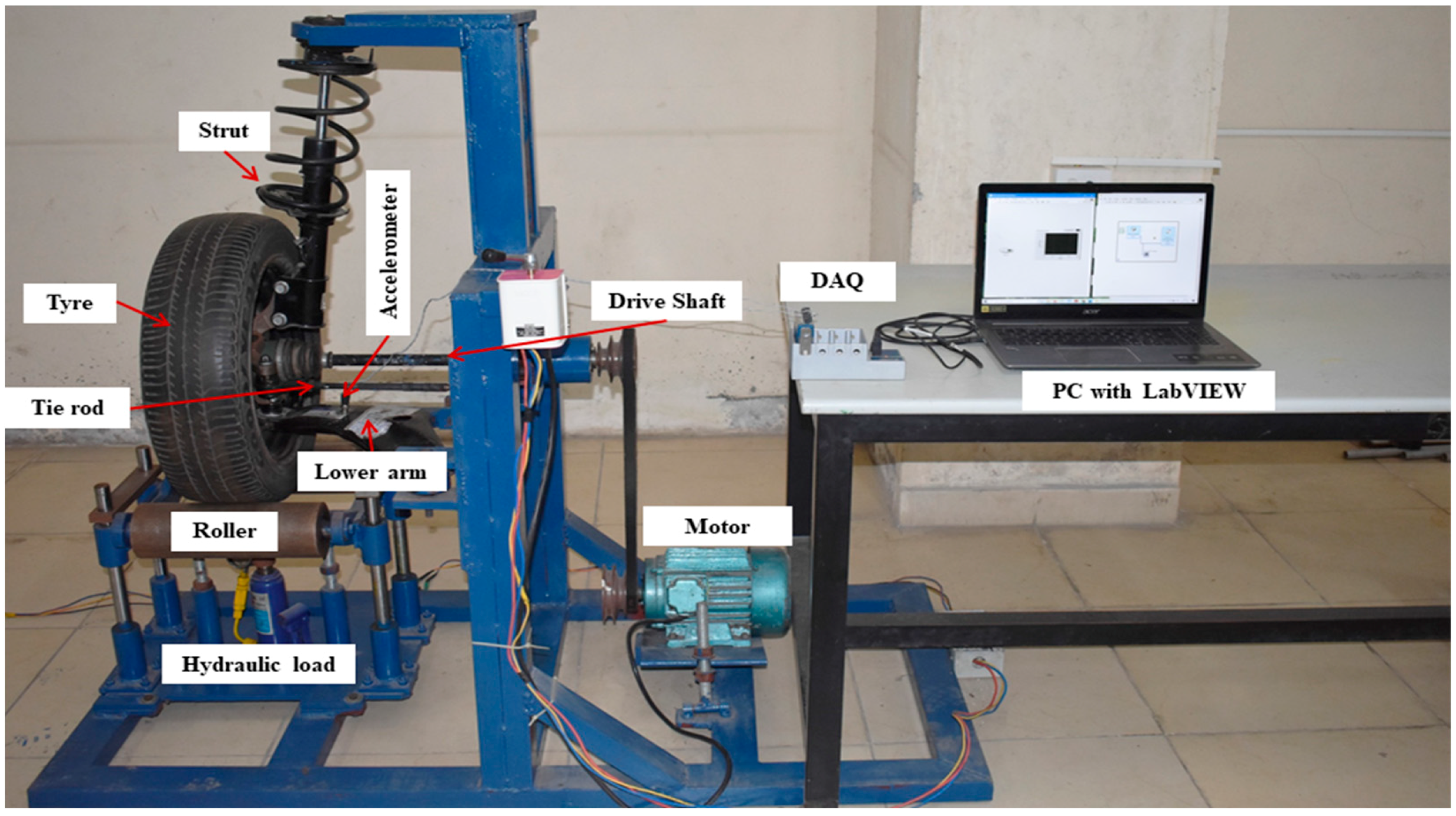
The experimental setup presented in Figure 3 comprises several essential components: a robust frame, a high-performance motor, a sturdy wheel, a durable driveshaft, an idle roller equipped with an efficient loading system and a McPherson suspension system. The suspension system comprises a shock absorber, an arm, a linkage rod and a wheel hub. A thoughtfully designed and carefully constructed experimental setup, resembling a model representing a quarter of a car, was ingeniously utilized to assess the performance of the suspension system. At the same time, the wheel moves along a smooth and evenly leveled surface at a constant velocity of 70 km/h. The constant speed of the wheel was achieved by placing it on two well-designed supporting rollers equipped with high-quality bearings that allow free rotation with minimal resistance. The motor with impressive power (in terms of rotational force) is harnessed using a sophisticated belt drive system coupled with reliable constant velocity joints to minimize the transmission of unwanted vibration to the system, thereby ensuring accurate and reliable testing results. In addition, the acting load on the suspension system is meticulously controlled via a highly advanced hydraulic system. The hydraulic system design facilitates the effortless height adjustment of the high-speed rollers, offering precise control over the load exerted on the suspension system. This thoughtfully crafted design ensures the suspension system is exposed to the exact and accurate force required to achieve the desired testing results.

2.2. Data Acquisition Method

Data acquisition involves collecting digital measurements of residual signals, such as vibration, temperature and sound, from a mechanical system’s real-time operating condition for analysis and visualization. The current study used a piezo-electric accelerometer (NI-PCB 352C03) with 10.26 mV/g sensitivity to acquire all the vibration signals for accurate system fault diagnosis. The accelerometer was mounted on the suspension system control arm using an adhesive technique. The accelerometer output signal was used as the input to the NI9234 Data acquisition system via a Universal Serial Bus (USB) chassis, and the NI LabVIEW software supported the data collection process. During the acquisition and storage of data, a few parameters and their values were considered. They are a sampling frequency of 25 kHz, a sample length of 10,000 steps and 100 instances for each class. The baseline load condition, “No Load” at 0 psi, indicates that the suspension system was in a state where the wheel was merely in contact with the roller. At the same time, power was transmitted to the wheel produced by the motor through the belt drive without the application of external force.

2.3. Experimental Procedure

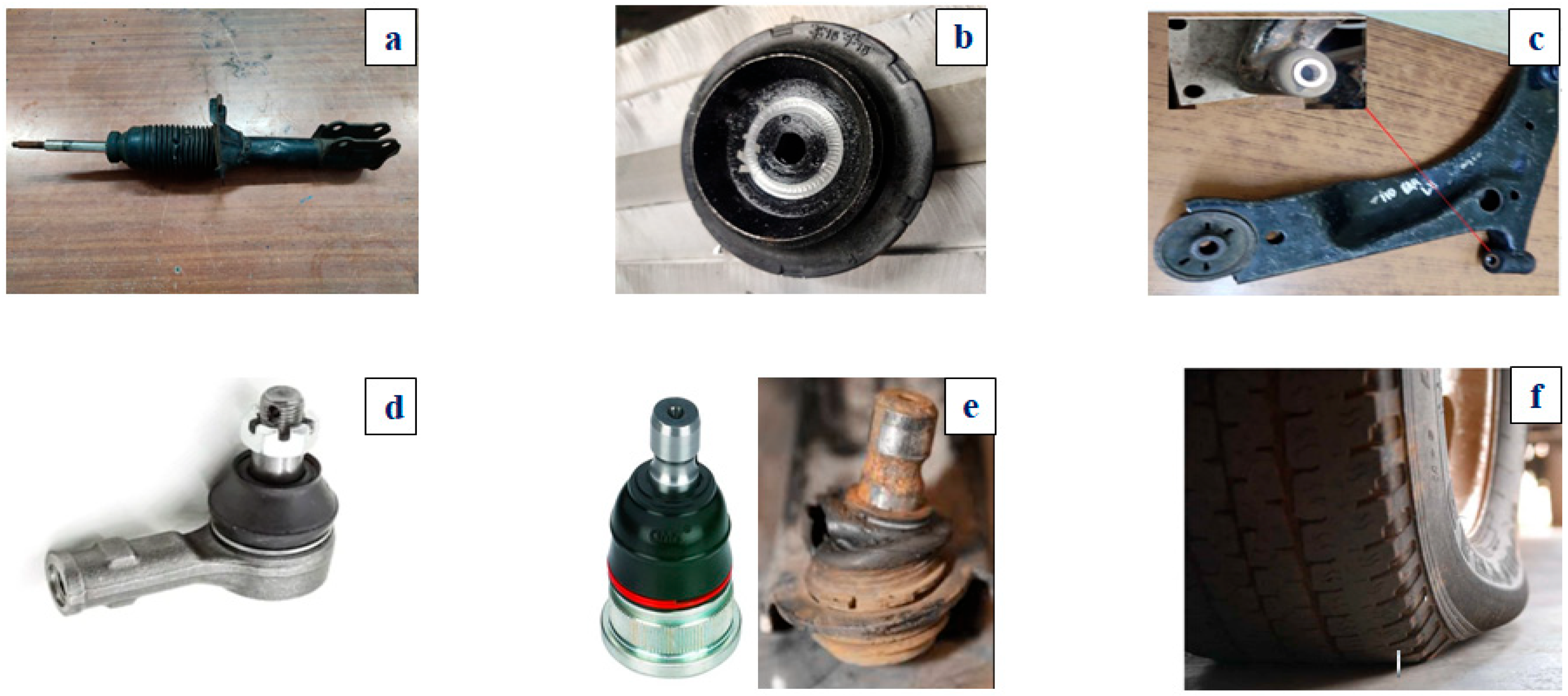
In the current study, the vibration readings from the suspension system were taken for eight cases and collected under no load conditions. A dataset of 100 signal samples was collected, each containing 10,000 data points via the accelerometer sensor. This process was repeated for all eight cases under study. These signals were then processed using Excel macros implemented with Visual Basic to generate radar plot images. The images were then locally saved and resized to meet the requirements of the pre-trained networks being used in the study. The resizing was done using a MATLAB algorithm, resulting in images with sizes of either 224 × 224 or 227 × 227 dimensions. The resized images were utilized as input data for training and classification purposes. By leveraging the power of the pre-trained networks, the study aimed to analyze and classify various fault conditions present in the suspension system. The images served as valuable visual representations of the underlying vibration patterns allowing the pre-trained networks to learn and make informed predictions. This experiment applies signal processing techniques, Excel macros and MATLAB algorithms to preprocess and transform raw vibration data into a format suitable for the pre-trained networks. The study aimed to enhance the understanding and classification accuracy of the suspension system fault condition by training these networks on the resized images. An overview of the discussed faults in this study is provided below, along with the pictorial representation (Figure 4).
  • Strut mount fault: The suspension system exhibits a fault in the strut mounting in which the connection and positioning of the strut mount are found to be defective.
  • Lower arm bush worn off: The bushing responsible for absorbing shocks and vibrations in the A-arm (also known as the control arm) has worn off. This can result in increased noise, reduced stability, and compromised handling of the suspension system.
  • The lower arm ball joint worn off: The fault occurs when the lower A-arm ball joint wears off. It can cause excessive play in the suspension, leading to abnormal tire wear, poor steering response and potential loss of control.
  • Tie rod ball joint worn off: This refers to when the joint connecting the steering rack to the steering knuckle wears off. It can result in unstable steering, vibration and difficulty maintaining proper wheel alignment.
  • Low pressure in the wheel: This refers to a situation where the tire pressure in one or more wheels is significantly lower than the recommended level. Insufficient tire pressure can lead to reduced handling, decreased stability, increased tire wear and decreased fuel efficiency.
  • Strut external damage: This refers to the condition wherein external damage to a strut, such as bends, dents or leaks, can compromise its structural integrity and affect the suspension’s ability to absorb shocks and maintain stability.
  • Strut worn off: This refers to the condition when a strut becomes worn off which can result in increased bouncing, reduced stability, longer stopping distances and an overall compromised ride quality.

3. Experimental Preprocessing and Analysis of Pre-Trained Networks

The primary objective of the present study was to preprocess and analyze radar plots showcasing accelerometer-acquired vibration signals generated in eight distinct suspension system conditions on a test bench.
These radar plots were resized and preprocessed into batches of either 224 × 224 pixels or 227 × 227 pixels. The transfer learning approach utilized the pre-trained networks trained on the ImageNet dataset. This approach allowed the models to learn from a large and diverse dataset, improving performance in handling the specific task. To adapt the pre-trained networks to handle the user-customizable dataset, to accommodate this particular user-customizable dataset, supplementary layers were incorporated to replace the existing output layers, aligning with the specific number of user-defined classes. The experimental preprocessing and analysis of the pre-trained networks included four different models: AlexNet, ResNet 50, VGG16 and GoogleNet. The comparative analysis of these four pre-trained networks, offering insights into their unique features and architectural designs, is presented in Table 3. This analysis provided valuable information on each model’s strengths and weaknesses. AlexNet, the first network to achieve a top-5 error rate below 20%, is a relatively shallow network with only eight layers and uses smaller filters than the later models, making it faster. ResNet 50, on the other hand, is a much deeper network, with 50 layers, making it more complex with higher accuracy. VGG16 is a deeper network consisting of 16 layers and employing a combination of smaller filters to improve accuracy. Lastly, GoogleNet employs a unique architecture of inception modules that reduces the number of parameters required for training, making it efficient and computationally inexpensive.

Formation of Dataset and Preprocessing

The current study utilized a dataset of images containing radar plots generated using signals in the time domain. The recorded vibration signals from the accelerometer were obtained and stored for the various conditions. These stored signals were reiterated using Microsoft Excel enabled with Visual Basics Macro to plot the radar images. 800 plots were generated, with each of the eight classes containing exactly 100 images. These images were processed further by resizing them to pixels according to the four chosen pre-trained networks. Figure 5 represents the various radar plot representations of the suspension conditions. Radar plots were adopted in the study due to ease of visualization, compactness, quick interpretability and multivariate comparison. These conditions included one standard and seven fault conditions, each represented by a unique set of radar plots. The generated plots were critical for analyzing the vibration data and provided valuable insights into the nature and severity of the different fault conditions. These insights could then be used to develop practical diagnostic and prognostic tools to enhance the performance and reliability of the suspension system.
Generally, radar plots are polygon-shaped in nature and represent data in a circular rather than linear form. The advantages of using radar plots over vibration plots is that radar plots converge the total information in a compact region. In contrast, horizontal vibration plots have information that occurs only in particular regions. Radar plots enhance the pattern learning capability of deep learning models over vibration plots. The original manuscript’s diagrams depict the images fed into the pre-trained models. The reason for doing so is to eradicate or biasing in classification due to the presence of external information such as axis details. The distance from the origin to each point in the plot represents the amplitude of the vibration signal while the axis ends represent the sample length, as shown in Figure 6.

4. Results and Discussion

The primary focus of this section is to comprehensively evaluate and compare the performance of the four selected pre-trained networks, namely VGG16, GoogleNet, AlexNet, and ResNet-50, aiming to conduct a thorough analysis for the fault detection of suspension systems. Various experimental settings were investigated to achieve this goal, including different train test data split ratios, solver algorithms, learning rates and batch sizes. The experiments were conducted by leveraging MATLAB R2022a software along with the necessary toolboxes, namely computer vision, transfer learning and deep learning. To provide a thorough account of the empirical observations, an extensive investigation of the efficacy of all four pre-trained networks under different experimental conditions was carried out. Specifically, the network accuracy varied with changes in the train to test split data ratio, solver, initial learning rate and batch size. A comparative analysis was conducted based on each network’s training time and model size under different experimental settings. The findings suggest that the choice of pretrained network and the experimental settings significantly affect fault detection performance in suspension systems. Among the four pre-trained networks, VGG-16 generally achieved peak precision, followed by GoogLeNet, ResNet-50 and AlexNet. However, the efficacy of each network varied depending on the experimental settings, with some networks performing better under certain conditions. A detailed description of all of the observations is presented in the sections below. The performance metric considered in the study for comparative purposes is test accuracy, which has been named classification accuracy in the following tables.

4.1. Impact of Train Test Ratio

In deep learning, training a neural network involves dividing the input data into two sets, the training and the testing data set. The training data set is used to update the biases of the neural network, while the testing data set is employed to evaluate the accuracy of the trained model. In the context of pre-trained networks, the same process is followed. The pre-trained network is first fine-tuned on the training dataset and then evaluated on the testing dataset. The train test data split ratio is the ratio in which the input/feed data are divided within these two sets. To identify the optimum train to test ratio for a particular pre-trained network, it is essential to experiment with different ratios and additional hyperparameters such as learning rate, solver method and batch size.
This study tested three differeg-testing data ratios for the four pretrained networks by keeping the remaining hyperparameters constant (batch size value of 10, solve algorithm as SGDM and a learning rate of 0.0001). The performance of each of the four pre-trained networks varies with a change in the train–train ratio, as shown in Table 4. For instance, AlexNet produced an accuracy of 90.60% at a train–test ratio of 0.80:0.20. VGG16 and GoogleNet produced 94.20% and 87.90% classification accuracy for 0.70:0.30 train-testing ratio. The ResNet-50 pretrained network achieved a maximum accuracy of 86.20% for the train to test ratio of 0.80:0.20. Therefore, the overall classification accuracies of the four networks at different split ratios were calculated as 88.83%, 92.56%, 88.80% and 85.60%, with the maximum overall accuracy being exhibited by VGG16.

4.2. Impact of Solvers

Deep learning is an ever-evolving field, and researchers are constantly seeking ways to improve the performance of DL models. One standard way to achieve this is by leveraging solvers, also known as optimizers. Solvers are various algorithms that minimize the value of training loss to improve the efficacy characteristics of the model during the process of training. In this study, three leading solvers were adopted to evaluate the performance of each of the four pre-trained networks. These are root mean square propagation (RMSprop), adaptive moment estimation (ADAM) and stochastic gradient descent (SGDM). The present study found that the optimum train–test split ratios for each of the pre-trained networks were as follows: for AlexNet, a split ratio of 0.80:0.20; for VGG16, a split ratio of 0.70:0.30; for GoogLeNet, a split ratio of 0.80:0.20; and for ResNet-50, a split ratio of 0.80:0.20. These ratios were found to yield higher classification accuracies for each respective model. However, it is essential to note that the choice of solvers can also influence the effectiveness of the pre-trained networks. As shown in Table 5, peak precision/accuracy was obtained by the GoogLeNet network with the RMSprop solver, achieving a massively high accuracy of 96.30% and an overall classification accuracy of 93.96%. In contrast, VGG16 had the lowest accuracy of 55.40% with the ADAM solver, which gave the lowest accuracy when compared with the accuracy obtained after the adoption of the SGDM solver (94.20%) as well as the RMSprop solver (67.90%). As a result, VGG-16 had the lowest overall classification accuracy of 72.50%, indicating that it was the worst performing network, with the lowest average accuracy percent considering all three solvers.

4.3. Impact of Batch Size

The choice of batch size during a deep neural network training significantly impacts its training dynamics and overall performance. Generally, larger batch sizes can speed up the training process by processing more samples per iteration. In comparison, smaller batch sizes can yield more accurate gradients and better generalization to unseen data. However, the optimal batch size can vary massively depending on the architecture and dataset. This study investigated the impact of batch size on the classification accuracy of four pre-trained neural network architectures (AlexNet, VGG-16, GoogLeNet and ResNet-50) using five different batch sizes of 8, 10, 16, 24 and 32 (Table 6). The experiment was conducted with the optimum hyperparameters identified in the previous section, including the optimizer and train–test ratio. The results showed that the optimal batch size varied depending on the architecture used. For the AlexNet architecture, a batch size of 16 resulted in the highest classification accuracy, while for VGG-16, GoogLeNet, and ResNet-50 architecture, 10 resulted in the highest classification accuracy. Specifically, ResNet-50 achieved the highest overall accuracy of 90.14%, with a maximum classification accuracy of 93.80% for the batch size of 10. The reason for these different optimal batch sizes can be attributed to the architecture and complexity of the neural network. For example, AlexNet has a relatively simple architecture compared to the other three networks and may benefit from larger batch sizes to speed up training. On the other hand, VGG-16, GoogLeNet and ResNet-50 have more complex architectures with deeper layers and may require smaller batch sizes to avoid overfitting and achieve better generalization. The choice of batch size also affects the memory usage of the neural network during training. Larger batch sizes require more memory to store the intermediate activations and gradients, which may become a limitation for GPUs with limited memory. On the other hand, smaller batch sizes may result in slower training due to the overhead of data transfer between the GPU and CPU.

4.4. Impact of Learning Rate

Choosing the appropriate initial learning rate is critical in achieving optimal model performance during training. For each update in the model weights, monitoring and supervising the changes in the model based on a predictable error is essential. However, choosing the ideal learning rate is not straightforward. It requires balancing the need for faster computation time and reducing the risk of high errors affecting the model’s accuracy. In this experiment, the researchers evaluated the impact of different initial learning rates of 0.0001, 0.0003 and 0.001 on the classification effectiveness of each network, keeping other hyperparameters constant for each network. The four pretrained networks performed differently based on the learning rate used, as shown in Table 7. The results show that the GoogLeNet network achieved the highest classification accuracy at an impressive 96.30% for a learning rate of 0.0001 but still ended up with the lowest overall accuracy of 78.76% in this comparison. This result is attributed to the fact that a lower learning rate helped to minimize the error value while keeping the computation time within reasonable limits. However, the optimal learning rate may vary depending on the choice of hyperparameters such as the optimizer algorithm and train to test ratio. For instance, the AlexNet network performed best with an SGDM solver and a 0.80:0.20 train to test ratio, while the VGG-16 network performed best with an SGDM solver and a 0.70:0.30 train to test ratio. On the other hand, the ResNet-50 and GoogLeNet networks performed best with an RMSprop solver and a 0.80:0.20 train to test ratio. Therefore, selecting an appropriate learning rate requires a balance between faster computation time and reducing the risk of high errors affecting the model’s accuracy. The results obtained from this experiment indicate that different networks may require different hyperparameters to achieve optimal performance during training. These findings underscore the importance of selecting appropriate solvers in achieving optimal performance in deep learning models. For instance, if VGG-16 were to be used in a classification task, it would be advisable to use the SGDM solver to obtain the highest possible classification accuracy. On the other hand, the RMSprop solver may be a better choice for other models, but it is important to note that this conclusion may vary according to the specific model in use and the task at hand.

4.5. Impact of Number of Epochs

The effect of epoch on CNNs is a crucial aspect to consider when training a model. The number of epochs determines how often the entire training dataset is run through the network during training. It plays a significant role in the convergence and overall performance of the model. To investigate the impact of different epoch values on the performance of a CNN, researchers trained multiple CNN architectures with varying epoch values and evaluated their classification performance. The other hyperparameters, such as learning rate, batch size and optimizer, were kept constant across all networks. The experiment revealed that the number of epochs directly influences the model’s accuracy. It was observed that as the number of epochs increased, the models initially showed improvements in accuracy; however, after reaching a certain point, they started to overfit the training data. Overfitting occurs when the model becomes too specialized in the training data and gives poor accuracy on new unseen data. The results indicated that an optimal number of epochs exists for each CNN architecture. Insufficient epochs may result in underfitting, where the model fails to effectively capture intricate patterns in the data. Conversely, excessive epochs can lead to overfitting, causing the model to “memorize” the data rather than “learn” generalizable features. Striking the right balance is crucial to ensure the model can grasp the underlying patterns in the data while avoiding excessive memorization. The researchers found that, as given in Table 8, VGG-16 architecture achieved the highest classification accuracy of 98.30% with 60 epochs, while GoogLeNet reached 96.30% accuracy with 10 epochs. The ResNet-50 architecture performed best with 40 epochs, achieving an accuracy of 96.20%. These results highlight the importance of selecting an appropriate number of epochs for each CNN architecture to achieve optimal performance. It is worth noting that the optimal number of epochs varies massively depending on the dataset and the sophistication level of the task. Therefore, it is crucial to experiment and fine-tune this hyperparameter for specific applications. The regular monitoring of the model’s performance on validation data can help determine the point at which the model starts to overfit, allowing for early stopping to prevent performance degradation.

4.6. Comparative Examination of Trained Models

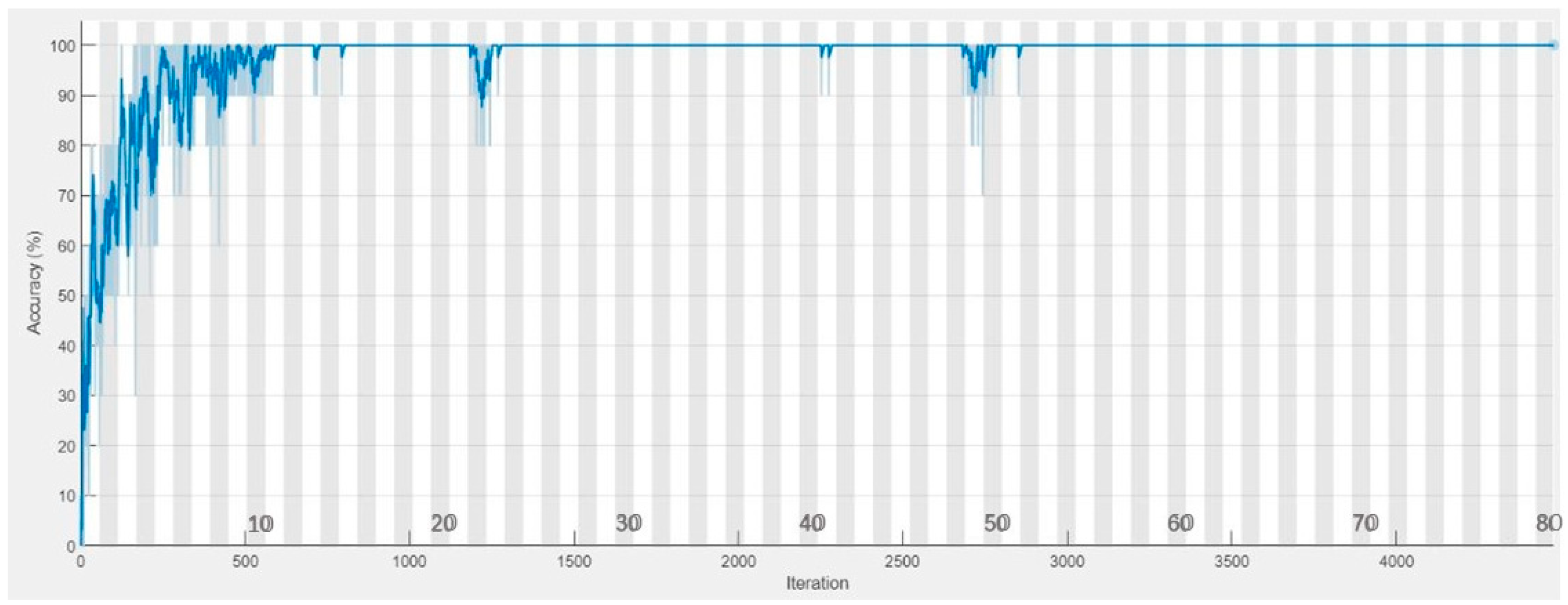
The current section delves into the effectiveness of pretrained networks and the selection of optimal hyperparameters that contribute to maximum classification accuracy. In this experimental research, the authors have prescribed the optimal hyperparameter settings, which have improved the overall effectiveness of pretrained models, in Table 9. Moreover, the performance/efficacy of pretrained networks with all the optimum hyperparameters is compared in Table 10. Analyzing the table reveals that VGG16 exhibits the highest accuracy when utilizing the observed optimal hyperparameters. Therefore, it is advised that VGG-16 be incorporated for fault detection in suspension systems, considering its superior classification accuracy. Figure 7 illustrates the training progress of VGG-16. The training curve demonstrates practical training as it reaches a plateau after the sixth epoch, indicating successful updates to the model weights. The reduction in data losses throughout the network training process further suggests the attainment of optimal hyperparameter choices.
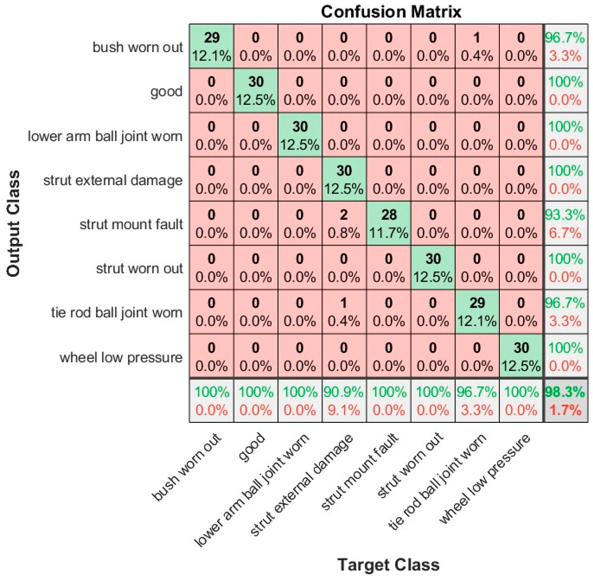
To further evaluate the performance of the VG16 architecture deployed in suspension system fault detection, Figure 8 presents a confusion matrix that visually illustrates the classification results obtained by the pre-trained network. This matrix offers an intuitive way to evaluate the network’s performance. By examining the diagonal elements, representing correctly classified instances, it becomes apparent that the network effectively transferred learning from the adopted network and minimized data loss during the learning process. Moreover, the absence of misclassified instances further confirms this observation. The confusion matrix is shown in Figure 8 and demonstrates that the architecture of VGG16 achieved a very high classification accuracy of 98.30%. Only four of the eight classes showed misclassifications. It is worth noting that these misclassifications may have been influenced by factors such as signal quality degradation, noise interference and similarities between acquired signals. Table 10 summarizes the optimized pretrained models’ performances, indicating that VGG16 outperformed the others. Considering its excellent performance, VGG16 is recommended as the most suitable and reliable pretrained DL network for malfunction detection in suspension systems.

4.7. Comparison with Other State of the Art Techniques

Multiple cutting-edge techniques were contrasted to prove the viability and dominance of the method proposed in this study over the other techniques for fault detection in suspension systems. Table 11 presents the final performance of other existing techniques (as well as of the proposed method). From Table 11, one can conclude that the method proposed in this study is superior due to its higher classification accuracy.
  • Bayes Net Classifier:
    -
    Balaji et al. [39] utilized the Bayes net classifier to detect faults in suspension systems.
    -
    Vibrational signals from a test bench were collected and used for classification.
    -
    The system was successfully classified into eight different conditions based on these signals.
  • Random Forest and J48 Algorithm:
    -
    Balaji et al. [40] employed the Random Forest and J48 algorithms for fault classification and detection in suspension systems.
    -
    The focus was on vibration signals, and the study investigated the system under eight distinct conditions.
  • Deep Semi-Supervised Feature Extraction:
    -
    Peng et al. [41] proposed a deep semi-supervised feature extraction method for fault detection in rail suspension systems.
    -
    This approach leveraged data from multiple sensors and was particularly effective when only one data class was available.
    -
    The study considered the system under two distinct conditions.
  • KNN (K-Nearest Neighbors), Naïve Bayes, Ensemble Methods, Linear SVM (Support Vector Machine):
    -
    Ankrah et al. [42] investigated the application of KNN, Naïve Bayes, ensemble methods, and linear SVM for fault detection in railway suspensions.
    -
    Acceleration signals were used for classification, and the system was classified into three different classes.
By examining the performance and capabilities of these techniques, in conjunction with the insights provided in Table 11, we can conclude that the proposed method is superior to other cutting-edge methods for fault detection in suspension systems.

5. Conclusions

This study aimed to investigate the effectiveness of transfer learning in the task of suspension system fault detection using four pretrained DL networks: GoogLeNet, VGG16, AlexNet and ResNet-50. The study focused on classifying seven primary suspension fault conditions (strut mount fault, A-arm bush worn off, lower A-arm ball joint worn off, tie rod ball joint worn off, low pressure in the wheel, strut external damage, strut worn off) and one normal reference state, based on analyzing vibration radar graphs. The trained networks used CNN layers to execute feature extraction, feature selection and classification in a unified manner, resulting in an end-to-end ML method. According to the study’s findings, transfer learning combined with ease of experimentation might be a viable solution for suspension system monitoring and the detection of defects. Statistical analysis showed that VGG16 produced the highest accuracy of 98.30%, followed by GoogLeNet, which yielded 96.30% accuracy, while AlexNet and ResNet-50 yielded an accuracy of 95.00% and 96.20%, respectively. VGG16 was chosen as the most optimally performing network and is recommended for performing suspension system fault detection economically. This entire procedure of fault detection in the suspension system with this method is speedy. This makes the model extremely viable to perform the task of fault detection. In terms of future scope, the proposed fault diagnosis system has the potential to be extended to handle multiple faults by integrating the superposition of sensors and accounting for varying speed conditions. Additionally, conducting real-time tests on the proposed method during vehicle operations, particularly for diagnosing suspension system faults using cruise control on a test track under constant load conditions, would yield valuable insights. Certain limitations do exist: the developed model works effectively for the acquired data; the acquisition or simulation of faults require expertise; data acquisition coupled with computational resources is a prime challenge. Finally, the study’s findings have important implications for developing modular and user-friendly defect diagnosis systems that might be implemented into commercially available vehicles for real-time detection.

Author Contributions

Conceptualization, S.A.S. and V.S.; methodology, S.N.V.; software, P.A.B.; validation, N.L., P.P. and S.D.; formal analysis, S.N.V. and V.S.; investigation, S.A.S., S.N.V. and V.S.; resources, P.A.B., N.L. and S.D.; data curation, P.A.B., S.N.V., P.P. and S.D.; writing—original draft preparation, S.N.V.; writing—review and editing, S.A.S., V.S. and S.D.; visualization, S.N.V., P.A.B. N.L., P.P. and S.D.; supervision, V.S. and S.D.; project administration, S.N.V., V.S. and S.D. All authors have read and agreed to the published version of the manuscript.

Funding

This research received no external funding.

Data Availability Statement

Data associated with the study can be obtained upon request from corresponding author.

Conflicts of Interest

The authors declare no conflict of interest.

References

  1. Liu, Y. Recent Innovations in Vehicle Suspension Systems. Recent Pat. Mech. Eng. 2012, 1, 206–210. [Google Scholar] [CrossRef]
  2. Fault Detection Methods: A Literature Survey. Available online: https://www.researchgate.net/publication/221412815_Fault_detection_methods_A_literature_survey (accessed on 8 June 2023).
  3. Lei, Y.; Yang, B.; Jiang, X.; Jia, F.; Li, N.; Nandi, A.K. Applications of Machine Learning to Machine Fault Diagnosis: A Review and Roadmap. Mech. Syst. Signal Process. 2020, 138, 106587. [Google Scholar] [CrossRef]
  4. Bellali, B.; Hazzab, A.; Bousserhane, I.K.; Lefebvre, D. Parameter Estimation for Fault Diagnosis in Nonlinear Systems by ANFIS. Procedia Eng. 2012, 29, 2016–2021. [Google Scholar] [CrossRef] [Green Version]
  5. Pouliezos, A.D.; Stavrakakis, G.S. Parameter Estimation Methods for Fault Monitoring. In Real Time Fault Monitoring of Industrial Processes; Springer: Berlin/Heidelberg, Germany, 1994; pp. 179–255. [Google Scholar] [CrossRef]
  6. Fagarasan, I.; Iliescu, S.S. Parity Equations for Fault Detection and Isolation. In Proceedings of the 2008 IEEE International Conference on Automation, Quality and Testing, Robotics, AQTR 2008—THETA 16th Edition—Proceedings, Cluj-Napoca, Romania, 22–25 May 2008; Volume 1, pp. 99–103. [Google Scholar] [CrossRef]
  7. Gertler, J.J. Structured Parity Equations in Fault Detection and Isolation. In Issues of Fault Diagnosis for Dynamic Systems; Springer: London, UK, 2000; pp. 285–313. [Google Scholar] [CrossRef]
  8. Zhao, W.; Lv, Y.; Guo, X.; Huo, J. An Investigation on Early Fault Diagnosis Based on Naive Bayes Model. In Proceedings of the 2022 7th International Conference on Control and Robotics Engineering, ICCRE 2022 2022, Beijing, China, 15–17 April 2022; pp. 32–36. [Google Scholar] [CrossRef]
  9. Asadi Majd, A.; Samet, H.; Ghanbari, T. K-NN Based Fault Detection and Classification Methods for Power Transmission Systems. Prot. Control. Mod. Power Syst. 2017, 2, 1–11. [Google Scholar] [CrossRef] [Green Version]
  10. Application of J48 Algorithm for Gear Tooth Fault Diagnosis of Tractor Steering Hydraulic Pumps. Available online: https://www.researchgate.net/publication/251881132_Application_of_J48_algorithm_for_gear_tooth_fault_diagnosis_of_tractor_steering_hydraulic_pumps (accessed on 8 June 2023).
  11. Yin, S.; Gao, X.; Karimi, H.R.; Zhu, X. Study on Support Vector Machine-Based Fault Detection in Tennessee Eastman Process. Abstr. Appl. Anal. 2014, 2014, 836895. [Google Scholar] [CrossRef] [Green Version]
  12. Aldrich, C.; Auret, L. Fault Detection and Diagnosis with Random Forest Feature Extraction and Variable Importance Methods. IFAC Proc. Vol. 2010, 43, 79–86. [Google Scholar] [CrossRef]
  13. Mishra, K.M.; Huhtala, K.J. Fault Detection of Elevator Systems Using Multilayer Perceptron Neural Network. In Proceedings of the IEEE International Conference on Emerging Technologies and Factory Automation, ETFA 2019, Zaragoza, Spain, 10–13 September 2019; pp. 904–909. [Google Scholar] [CrossRef]
  14. Zhu, X.; Xia, Y.; Chai, S.; Shi, P. Fault Detection for Vehicle Active Suspension Systems in Finite-Frequency Domain. IET Control. Theory Appl. 2019, 13, 387–394. [Google Scholar] [CrossRef]
  15. Azadi, S.; Soltani, A. Fault Detection of Vehicle Suspension System Using Wavelet Analysis. Veh. Syst. Dyn. 2009, 47, 403–418. [Google Scholar] [CrossRef]
  16. Börner, M.; Isermann, R.; Schmitt, M. A Sensor and Process Fault Detection System for Vehicle Suspension Systems. Available online: https://books.google.com.hk/books?hl=en&lr=&id=auGbEAAAQBAJ&oi=fnd&pg=PA103&dq=Sensor+and+Process+Fault+Detection+System+for+Vehicle+Suspension+Systems&ots=xDSZYcKAgA&sig=y1LgiX6LS6lvPRiGBLg2Nug9elk&redir_esc=y#v=onepage&q=Sensor%20and%20Process%20Fault%20Detection%20System%20for%20Vehicle%20Suspension%20Systems&f=false (accessed on 8 June 2023).
  17. Liu, C.; Gryllias, K. A Semi-Supervised Support Vector Data Description-Based Fault Detection Method for Rolling Element Bearings Based on Cyclic Spectral Analysis. Mech. Syst. Signal Process 2020, 140, 106682. [Google Scholar] [CrossRef]
  18. Vasan, V.; Sridharan, N.V.; Prabhakaranpillai Sreelatha, A.; Vaithiyanathan, S. Tire Condition Monitoring Using Transfer Learning-Based Deep Neural Network Approach. Sensors 2023, 23, 2177. [Google Scholar] [CrossRef]
  19. Chakrapani, G.; Sugumaran, V. Transfer Learning Based Fault Diagnosis of Automobile Dry Clutch System. Eng. Appl. Artif. Intell. 2023, 117, 105522. [Google Scholar] [CrossRef]
  20. Tang, S.; Yuan, S.; Zhu, Y. Deep Learning-Based Intelligent Fault Diagnosis Methods toward Rotating Machinery. IEEE Access 2020, 8, 9335–9346. [Google Scholar] [CrossRef]
  21. Jegadeeshwaran, R.; Sugumaran, V. Fault Diagnosis of Automobile Hydraulic Brake System Using Statistical Features and Support Vector Machines. Mech. Syst. Signal Process 2015, 52–53, 436–446. [Google Scholar] [CrossRef]
  22. Ding, A.; Qin, Y.; Wang, B.; Jia, L.; Cheng, X. Lightweight Multiscale Convolutional Networks with Adaptive Pruning for Intelligent Fault Diagnosis of Train Bogie Bearings in Edge Computing Scenarios. IEEE Trans Instrum Meas 2023, 72, 3231325. [Google Scholar] [CrossRef]
  23. Tanyildizi, H.; Şengür, A.; Akbulut, Y.; Şahin, M. Deep Learning Model for Estimating the Mechanical Properties of Concrete Containing Silica Fume Exposed to High Temperatures. Front. Struct. Civ. Eng. 2020, 14, 1316–1330. [Google Scholar] [CrossRef]
  24. Ai, D.; Mo, F.; Cheng, J.; Du, L. Deep Learning of Electromechanical Impedance for Concrete Structural Damage Identification Using 1-D Convolutional Neural Networks. Constr. Build Mater. 2023, 385, 131423. [Google Scholar] [CrossRef]
  25. Fraz, M.M.; Jahangir, W.; Zahid, S.; Hamayun, M.M.; Barman, S.A. Multiscale Segmentation of Exudates in Retinal Images Using Contextual Cues and Ensemble Classification. Biomed. Signal Process Control 2017, 35, 50–62. [Google Scholar] [CrossRef] [Green Version]
  26. Mo, J.; Zhang, L.; Feng, Y. Exudate-Based Diabetic Macular Edema Recognition in Retinal Images Using Cascaded Deep Residual Networks. Neurocomputing 2018, 290, 161–171. [Google Scholar] [CrossRef]
  27. Ansari, A.H.; Cherian, P.J.; Caicedo, A.; Naulaers, G.; De Vos, M.; Van Huffel, S. Neonatal Seizure Detection Using Deep Convolutional Neural Networks. Int. J. Neural Syst. 2019, 29, 1850011. [Google Scholar] [CrossRef] [Green Version]
  28. Nogay, H.S.; Adeli, H. Detection of Epileptic Seizure Using Pretrained Deep Convolutional Neural Network and Transfer Learning. Eur. Neurol 2021, 83, 602–614. [Google Scholar] [CrossRef]
  29. Zhang, Y.; You, D.; Gao, X.; Zhang, N.; Gao, P.P. Welding Defects Detection Based on Deep Learning with Multiple Optical Sensors during Disk Laser Welding of Thick Plates. J. Manuf. Syst. 2019, 51, 87–94. [Google Scholar] [CrossRef]
  30. Zhang, Z.; Wen, G.; Chen, S. Weld Image Deep Learning-Based on-Line Defects Detection Using Convolutional Neural Networks for Al Alloy in Robotic Arc Welding. J. Manuf. Process 2019, 45, 208–216. [Google Scholar] [CrossRef]
  31. Shao, H.; Jiang, H.; Zhang, X.; Niu, M. Rolling Bearing Fault Diagnosis Using an Optimization Deep Belief Network. Meas. Sci. Technol. 2015, 26, 115002. [Google Scholar] [CrossRef]
  32. Huang, W.; Cheng, J.; Yang, Y.; Guo, G. An Improved Deep Convolutional Neural Network with Multi-Scale Information for Bearing Fault Diagnosis. Neurocomputing 2019, 359, 77–92. [Google Scholar] [CrossRef]
  33. Li, X.; Jiang, H.; Niu, M.; Wang, R. An Enhanced Selective Ensemble Deep Learning Method for Rolling Bearing Fault Diagnosis with Beetle Antennae Search Algorithm. Mech. Syst. Signal Process 2020, 142, 106752. [Google Scholar] [CrossRef]
  34. Liu, G.; Bao, H.; Han, B. A Stacked Autoencoder-Based Deep Neural Network for Achieving Gearbox Fault Diagnosis. Math Probl. Eng. 2018, 2018, 5105709. [Google Scholar] [CrossRef] [Green Version]
  35. Naveen Venkatesh, S.; Chakrapani, G.; Senapti, S.B.; Annamalai, K.; Elangovan, M.; Indira, V.; Sugumaran, V.; Mahamuni, V.S. Misfire Detection in Spark Ignition Engine Using Transfer Learning. Comput. Intell Neurosci. 2022, 2022, 7606896. [Google Scholar] [CrossRef]
  36. Zhao, W.; Wang, Z.; Lu, C.; Ma, J.; Li, L. Fault Diagnosis for Centrifugal Pumps Using Deep Learning and Softmax Regression. In Proceedings of the World Congress on Intelligent Control and Automation (WCICA), Guilin, China, 12–15 June 2016; Institute of Electrical and Electronics Engineers Inc.: Piscataway, NJ, USA, 2016; Volume 2016, pp. 165–169. [Google Scholar]
  37. Shao, S.Y.; Sun, W.J.; Yan, R.Q.; Wang, P.; Gao, R.X. A Deep Learning Approach for Fault Diagnosis of Induction Motors in Manufacturing. Chin. J. Mech. Eng. Engl. Ed. 2017, 30, 1347–1356. [Google Scholar] [CrossRef] [Green Version]
  38. Helbing, G.; Ritter, M. Deep Learning for Fault Detection in Wind Turbines. Renew. Sustain. Energy Rev. 2018, 98, 189–198. [Google Scholar] [CrossRef]
  39. Arun Balaji, P.; Sugumaran, V. A Bayes Learning Approach for Monitoring the Condition of Suspension System Using Vibration Signals. IOP Conf. Ser. Mater. Sci. Eng. 2021, 1012, 012029. [Google Scholar] [CrossRef]
  40. Arun Balaji, P.; Sugumaran, V. Fault Detection of Automobile Suspension System Using Decision Tree Algorithms: A Machine Learning Approach. Proc. Inst. Mech. Eng. Part E J. Process Mech. Eng. 2023, 09544089231152698. [Google Scholar] [CrossRef]
  41. Peng, X.; Jin, X. Rail Suspension System Fault Detection Using Deep Semi-Supervised Feature Extraction with One-Class Data. Annu. Conf. PHM Soc. 2018, 10, 546. [Google Scholar] [CrossRef]
  42. Ankrah, A.A.; Kimotho, J.K.; Muvengei, O.M.; Ankrah, A.A.; Kimotho, J.K.; Muvengei, O.M. Fusion of Model-Based and Data Driven Based Fault Diagnostic Methods for Railway Vehicle Suspension. J. Intell. Learn. Syst. Appl. 2020, 12, 51–81. [Google Scholar] [CrossRef]
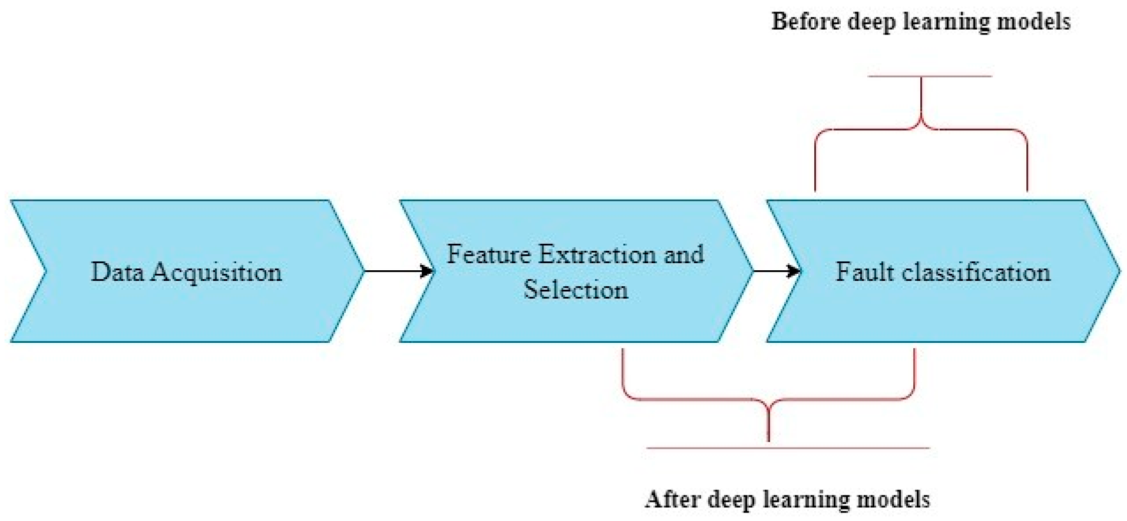
Figure 1. Scenario depicting the impact of DL models.
Machines 11 00778 g001
Figure 2. Flowchart illustrating the steps undertaken in the present study.
Machines 11 00778 g002
Figure 3. The adopted experimental setup in the present study.
Machines 11 00778 g003
Figure 4. (a) strut mount failure (b) strut external damage (c) lower arm bush worn out (d) lower arm ball joint fault (e) strut worn out and (f) low tire pressure.
Machines 11 00778 g004
Figure 5. Radar plot samples depicting all eight conditions of the suspension system (a) good (b) lower arm ball joint worn off (c) strut mount fault (d) strut worn off (e) tie rod ball joint worn off (f) strut external damage (g) low pressure in the wheel (h) lower arm bush worn off.
Machines 11 00778 g005
Figure 6. Sample radar plot depicting amplitude (distance from origin) and sample length (at each axis end).
Machines 11 00778 g006
Figure 7. Training progress plot of VGG16 Pretrained Network.
Machines 11 00778 g007
Figure 8. Confusion matrix of VGG16 Pretrained Network.
Machines 11 00778 g008
Table 1. Models suggested in the literature for the fault diagnosis of the suspension system.
Model TypeName of the Model Working PrincipleReference
MathematicalParameter EstimationThis model employs ordinary differential equations to find multiple parameters that portray variations when a fault is detected. These parameters are then compared to the optimal set, and the error is found[4,5]
Parity equations with input/output modelsThis model employs the transfer function to find the output and polynomial error between the model and output[6,7]
Machine LearningNaive BayesThis model uses a machine learning algorithm for classification using the Bayes theorem. This classifier assumes strong independence between the features[8]
kNNKNN does not rely on any specific assumptions, earning its reputation as a non-parametric algorithm[9]
J48This algorithm results from improving and implementing the C4.5 algorithm[10]
SVMSVM is another famous ML algorithm that forms a hyperplane to classify data[11]
Random ForestThe random forest algorithm employs multiple decision trees on subsets of the given data to improve the model’s and the dataset’s predictive accuracy[12]
MLPMLP or Multilayer Perceptron is a model which uses the back propagations algorithm to classify data[13]
Table 3. Characteristics of pre-trained networks used in this study.
NetworkNumber of LayersKey FeaturesInput SizeTraining Time
AlexNet8 layers (5 convolutional, 3 fully connected)-Introduced the concept of deep learning for image classification227 × 227Medium
-Utilized rectified linear units (ReLU) for non-linearity
-Used dropout regularization
-Implemented local response normalization
GoogleNet22 layers (27 including auxiliary classifiers)-Introduced the concept of inception modules224 × 224High
-Utilized 1 × 1 convolutions to reduce the computational cost
-Used global average pooling for dimensionality reduction
-Employed multiple auxiliary classifiers for training
VGG1616 layers (13 convolutional, 3 fully connected)-Utilized small 3 × 3 convolutional filters throughout224 × 224High
-Maintained a simple and uniform architecture
-Achieved impressive performance on various image classification tasks
-Increased depth with multiple convolutional layers
ResNet5050 layers (49 convolutional, 1 fully connected)-Introduced residual connections to address vanishing gradient problem224 × 224High
-Utilized skip connections to pass activations forward
-Enabled training of intense neural networks
-Introduced the concept of residual blocks
Table 4. Accuracy of pretrained networks at various split ratios.
Pretrained ModelClassification Accuracy for Different Split Ratio (%)Mean Accuracy
(%)
0.70:0.300.75:0.250.80:0.20
VGG-1694.2093.5090.0092.56
GoogLeNet87.9086.0092.5088.80
AlexNet90.4085.5090.6088.83
ResNet-5084.6086.0086.2085.60
Table 5. Accuracy of pre-trained networks for different optimizers (solvers).
Pretrained ModelClassification Accuracy for Different Solvers (%)Mean Accuracy
(%)
SGDMADAMRMSPROP
VGG-1694.2055.4067.9072.50
GoogLeNet92.5093.1096.3093.96
AlexNet90.6082.5089.4087.50
ResNet-5086.2090.0093.8090.00
Table 6. Accuracy of pre-trained networks for the 5 different batch sizes.
Pretrained ModelClassification Accuracy at Different Batch Sizes (%)Mean Accuracy
(%)
810162432
VGG1689.6094.2091.7092.9079.6089.60
GoogLeNet90.0096.3094.4090.0069.4088.02
AlexNet90.0090.6091.9085.6090.6089.74
ResNet-5091.9093.8091.9090.0083.1090.14
Table 7. Accuracy of pre-trained networks for different initial learning rates.
Pretrained ModelClassification Accuracy for Different Learning Rates (%)Mean Accuracy
(%)
0.00010.00030.001
VGG-1694.2086.7080.8087.23
GoogLeNet96.3090.0050.0078.76
AlexNet91.9092.5088.1090.83
ResNet-5093.8083.8081.2086.26
Table 8. Accuracy of pre-trained networks for different numbers of epochs.
Pretrained ModelClassification Accuracy for Different Numbers of Epochs (%)Mean Accuracy
(%)
102030405060708090100
VGG-1694.2095.0096.7095.0096.7098.3097.9097.1097.2095.8096.39
GoogLeNet96.3095.6095.3069.4095.0094.3894.3092.5090.6091.6091.49
AlexNet92.5088.8093.8092.5095.0094.4094.2093.1092.2090.0092.65
ResNet-5093.8091.9091.2096.2095.1095.6086.9094.3086.2084.4091.67
Table 9. Optimal hyperparameters for all four of the pretrained models.
Pretrained ModelOptimal Hyperparameter Configuration
Split RatioSolverBatch SizeLearning RateEpochs
VGG-160.70:0.30SGDM100.000160
GoogLeNet0.80:0.20RMSprop100.000110
AlexNet0.80:0.20SGDM160.000350
ResNet-500.80:0.20RMSprop100.000140
Table 10. Comparative analysis of the performance among diverse pre-trained networks with their optimal hyperparameters.
Pretrained ModelMaximum Classification Accuracy Achieved
(%)
VGG-1698.30
GoogLeNet96.30
AlexNet95.00
ResNet-5096.20
Table 11. Comparative analysis of accuracy between proposed method and state of the art techniques.
ReferenceTechnique UsedTotal Number of ConditionsTypes of Plots/SignalsAccuracy (%)
[39]Bayes Net Machine learning classifier8Vibrational Signals88.40
[40]Random Forest8Vibration Signals95.88
J48 Algorithm 94.00
[41]Deep Semi Supervised method2Multi Sensor data85.00
[42]KNN3Acceleration Signals71.90
Naïve Bayes78.10
Ensemble81.30
Linear SVM84.40
Proposed Method8Vibration signals with radar plots98.30
Disclaimer/Publisher’s Note: The statements, opinions and data contained in all publications are solely those of the individual author(s) and contributor(s) and not of MDPI and/or the editor(s). MDPI and/or the editor(s) disclaim responsibility for any injury to people or property resulting from any ideas, methods, instructions or products referred to in the content.