Mechanical Design of a 2-PRR Parallel Manipulator for Gait Retraining System

Abstract

Robotic gait retraining systems typically function by employing mechanisms that move a patient’s lower limbs in a controlled manner. In this paper, an end-effector gait retraining system was designed, utilizing a 2-PRR mechanism (PRR refers to the structure of each robot’s limb, consisting of an active prismatic pair (P) and two passive rotational pairs (RR) pairs). The mechanism, which corresponds to a parallel robot, was synthesized through visual design tools (design atlases) to evaluate performance indices, such as the workspace size, local and global conditioning, and mechanism stiffness. Quasi-static force analyses were conducted to calculate worst-case scenario operational loads. These loads were then used to obtain a valid cross-section geometry that would withstand static stress, buckling failure, and fatigue failure.

1. Introduction

1.1. Motivation

The study of robot-assisted gait rehabilitation systems has increased in popularity as a way to reduce exercise irregularities in therapy sessions and alleviate the physical strain put upon therapists by automating specific processes [1,2]. Most physically-implemented robot-assisted gait rehabilitation systems fall into two categories: end-effector and exoskeleton-based approaches [3].

Lower-limb robotic exoskeletons can help individuals with mobility impairments to perform gait exercises by providing additional force and torque to compensate for muscle weakness or other health conditions. Exoskeletons intervene directly upon the principal joints that allow for the movement of the lower limbs: the hip, knees, and ankles, all of which are regions that lose functionality with age, injuries, or health conditions. As described in [4], there are many different types of exoskeletons, depending on the health conditions that the target users could have. For example, the Lokomat system is an exoskeleton used with a treadmill to assist with the robotic rehabilitation of locomotion [5]. This system tests the sensory afferent modulation of different reflexes and carries out electromyogram studies. Similar systems have been designed under the same principles, such as the LOPES gait trainer [6] and other systems that have similar design principles, such as the Berkeley Lower Extremity Exoskeleton (BLEEX) [7]. Other groups have sought to monitor force using soft sensors integrated into lower-limb exoskeletons [8]. After testing the soft sensor under different torque profiles, the results showed that mistiming the interaction force between the exoskeleton and the lower limbs could further hinder the patient’s movements with the exoskeleton. Recently, a research group at the University of Tsukuba designed a knee brace device to mitigate a specific type of pathological gait in individuals with cerebral palsy [9]. By applying a braking torque to the knee, this device could reduce unnatural hip flexion and detect the activation of certain essential muscle groups. Some recent advances in lower limb exoskeleton-based rehabilitation systems include a 6-DoF system developed by the Indian Institute of Technology that controls the thigh, shank, and foot in the plane [10]. This system was designed for children aged 8–12, and an external walker-like frame for increased stability on flat terrains supported the mechanism. Due to lower mass, torque, and power requirements, significant power sources were not needed. Another system includes a 4-DoF 3-PRRR parallel configuration for complete spatial control of lower limbs [11]. This system has the patient in a fixed position in a reclined chair while the mechanisms actuate each lower limb. Others present kinematic models of a pneumatic-actuated exoskeleton based on biomechanical data and anthropometrical parameters [12]. The geometric model serves as a base for the future design of a gait retraining system.

End-effector-based gait retraining systems function using footplates that simulate the position of extremities in the stance and swing phase [13]. Footplate-based systems are typically used for early-stage rehabilitation, where the user is bedridden or wheelchair-bound. These systems do not have the user in contact with the ground or a treadmill. Instead, only the user’s feet are attached to the gait retraining system [3]. One of the first end-effector-based gait retraining systems was proposed in 1999 [13,14], which later paved the way for various end-effector systems, such as the Haptic Walker system [15] and its commercial successor, the G-EO gait robot [16]. Both end-effector and exoskeleton-based systems use Body-Weight Support (BWS), such as harnesses, to help balance the user and displace the body’s center of mass.

In general, exoskeletons are more complex than end-effector systems, as they interact directly with each limb’s segment, implying interference and friction, which require multiple joints and actuators to comfortably reproduce the natural human movements of the legs during walking [17]. The control system for an exoskeleton must monitor the patient’s real-time gait, including the range of motion and joint torque requirements, and adjust the level of assistance the exoskeleton provides accordingly. Consequently, the control of exoskeletons requires sophisticated algorithms and advanced sensors to ensure that the system responds appropriately to the patient’s movement, e.g., regarding the exoskeleton system shown in [18]; this system needs cumbersome off-board actuation units that provide power to a processing unit that monitors ground reaction force, kinematic data, and metabolic data and powers the exoskeleton itself. On the other hand, in end-effector systems, continuous feedback of reactive force is not necessary because of the closed-loop kinematic system’s nature. Because of this, researchers such as [17,19] found that end-effector systems are typically more cost-effective in a clinical setting than analogous exoskeleton-based systems. The kinematic models of end-effector systems are also associated with simpler motion control schemes compared to exoskeleton systems [20].

Despite the benefits of end-effector-based systems, there are limitations. First, like any other assistive device, end-effector systems depend on specific disabilities that vary significantly from one patient to another [21]. Second, many systems repeat a kinematically preprogrammed trajectory [17,21], making them static and non-parameterizable. Finally, while end-effector systems have increased stability and there is less risk of falling compared to an exoskeleton system [22,23], this is at the cost of being less portable [23,24]. Some suggest that these pros and cons make end-effector-based systems better suited for static rehabilitation therapy and less useful for non-monitored day-to-day assistance [24].

Most of the gait retraining systems previously mentioned have many Degrees of Freedom (DoFs), which require an elaborate control strategy [25]. Certain institutions have synthesized low DoFs mechanisms for end-effector-based gait retraining systems. The University of California in Irvine used a one-DoF Stephenson III linkage to help guide and develop the relative trajectory of the ankle relative to the hip [26]. A similar system was designed by Tianjin University, using cam-linkage mechanisms for individual therapy rather than generalized treatment at rehabilitation centers; however, the use of a pantograph mechanism was to be studied to scale the generated trajectory in terms of patient anthropometry [27]. These systems restrain the movement of each extremity in a plane parallel to the sagittal plane.

1.2. Parallel Manipulators

Parallel manipulators are an alternative for generators of precise, high-speed motion under severe dynamic loading [28,29]. The dimensional synthesis of parallel manipulators uses kinematic models to evaluate performance indices. These indices can express information about the desired work-space, conditioning or isotropy, stiffness, and singularities (or other Jacobian-based variables) as a function of mechanism geometry [30].

Liu and Wang have proposed the Parameter-Finiteness Normalization Method (PFNM) to reduce the number of independent parameters to solve for [31]. PFNM is a helpful tool when designing parallel robots with reduced DoFs and dimensional parameters. A mechanism with three-dimensional parameters can be expressed as two non-dimensional independent parameters, which allow visualization of all design indices through design atlases (2D colormaps). This process is called the Performance-Chart-based Design Methodology (PCbDM) [28,31].

Parallel robots have been used to design some gait retraining and gait rehabilitation systems. Mohan and coworkers [32] designed a three-DoFs parallel robot with a 2PRP-2PPR structure that was combined with an adjustable seat and a passive orthosis to obtain a programmable gait trajectory restricted to the sagittal plane. This paper presents the design stage, kinematic and dynamic models, motion and control design, and performance evaluation. Mohanta et al. [33] proposed a three-DoFs planar parallel manipulator focused on a footplate motion control in the sagittal plane. Similar to [32], the design incorporates the adjustable seat and passive orthosis. The motion control of the device was addressed in [34]. The G-EO system that was mentioned earlier is a parallel-robot-based design that advanced to the commercial stage. The design is based on closing a kinematic chain from the hip to the ankle attached to the robot end-effector. Given the kinematic constraints, controlling the ankle trajectory results in the required motion of the limb. Regarding one limb, the robot has two DoFs, corresponding to two prismatic driving links that control a dyad (a kinematic chain formed by two links and three rotational pairs). The ankle’s trajectory is constrained to the sagittal plane. An additional rotational pair independently controls the ankle orientation. Hesse et al. [16] present a complete description of the system.

A common characteristic of the reviewed parallel robots for gait retraining is the reduced DoFs and the number of kinematic parameters (length of links), allowing the use of PFNM and PCbDM in the kinematic synthesis process.

1.3. Proposed System

The anthropometric parameters that take part in human gait can be complex. These parameters and characteristics lead to multiple design considerations that can vary depending on the lower-limb segments that are analyzed [35]. One possible design solution is to focus on the ankle trajectory and create a device that can replicate its kinematics, actively move the joint, and consequently move the knee and hip, thus generating the complete gait pattern in the sagittal plane. For this to function, the hip must be fixed and the knee must have support to avoid movements outside of the sagittal plane. However, these supports are outside the core of this discussion.

An interdisciplinary group of researchers of the Universidad Autónoma de Manizales established systematically weighted criteria for designing and developing mechanisms that could model the trajectory of the ankle joint that make up the end-effector gait retraining system in the sagittal plane; this was carried out following the weighted-objective method presented by [36]. The workgroup consisted of three physiotherapists, one biomedical engineer, one mechanical engineer, two electronic engineers, two industrial designers, and undergraduate physiotherapy, mechanical engineering, and biomedical engineering students. The decision to design an end-effector system was based on studies that have shown that end-effector-based systems have more beneficial results in clinical trials than exoskeletons when evaluating walking speed, endurance, and metabolic energy consumption [37,38]. Additionally, other studies have declared that most exoskeleton-based systems currently available have the disadvantages of being bulky and difficult to use, and some are even equipped with components, such as a power source, that bring discomfort for the wearer [39,40].

Some criteria can be evaluated quantitatively based on mathematical models. Other criteria, however, are more Boolean; in this case, criteria were evaluated based on whether they were present or not in the design. The importance of each criterion can then weigh relative scores. After following the weighted-objective method, each researcher proposed what he or she considered the adequate weight for each criterion; these percentage weights were then averaged between the whole research group for the final criteria evaluation weights registered in

Table 1. Criteria and evaluation weight.

Criteria	Defined Weight
C1—Reprogrammability	20.83%
C2—Adjustability to different anthropometries	22.67%
C3—Easy implementation of a control system	13.17%
C4—Need for a harness or additional trunk support	13.75%
C5—Independent control of each lower limb	15.83%
C6—Variable levels of assistance	13.75%

[36].

With these criteria, five alternatives were proposed with different advantages and qualities compared with one another, where each end-effector alternative was meant to model the trajectory of the ankle relative to the hip, resulting in the expected kinematics for the knee and hip. Only five alternatives were chosen to facilitate the evaluation of the decision matrix, as presented in

Table 2. Possible mechanism alternatives and final score from decision matrix.

Alternative	Global Score
A1—Stephenson III mechanism	5.87
A2—Cam-linkage mechanism	5.79
A3—Slider-crank 7 bar mechanism	7.29
A4—2-PRR mechanism	7.58
A5—2-PRR mechanism with extra DoF for foot orientation	7.53

.

With the scores presented in Table 2, the type synthesis was finalized, and it was determined that the 2-PRR mechanism was the most valid alternative according to the previously established requirements. PRR refers to the kinematic structure of each robot’s limb, consisting of an active prismatic pair (P) and two passive rotational pairs (RR).

With this taken into account, the design of a two-DoFs parallel manipulator for a BWS-end-effector-based gait retraining system was presented. The dimensional synthesis of the 2-PRR parallel manipulator takes into account the mechanism work-space $\left(w_t\right)$, Minimum Characteristic Length $\left(R_{\min }\right)$, Global Conditioning Index $\left(GCI\right)$, Maximum Local Conditioning Index $\left(MCI\right)$, and Global Stiffness Index $\left(GSI\right)$. This work took place in Colombia, where some of these systems are being studied and applied in academia [41,42]; however, commercial options are often limited. Imported exoskeleton and end-effector gait retraining systems can be found in certain rehabilitation centers; however, due to their high costs, it is not very viable for most people to have access to the services that these systems bring. This creates the necessity to design a more viable gait retraining system in the socio-economic context that most people with disabilities face in Colombia. The potential benefits of this new system are the following:

• Has fewer DoFs than most commercial options, which could lead to a more economic system due to having fewer actuators.
• The kinematics of the system is relatively simple to control.
• VR task-oriented exercises can be conducted simultaneously while gait retraining.
• Assists the demand for gait retraining systems in Colombia.
• Even if the design context is specific, it could be transposed to a similar context overseas, e.g., in Latin American countries.

Therefore, while other systems based on parallel robotics are present, the novelty of this work is evidenced in:

• A reduced number of DoFs to control the ankle’s trajectory, similar to [16], is achieved.
• A detailed description of dimensional synthesis based on kinematical performance indices, which other studies do not explicitly report [5,16]. Involving performance indices in the synthesis improves the design robustness, e.g., augmenting the workspace and dexterity with sufficient stiffness. Even when no inertial parameters are determined in this stage, a kinematically-assessed design promotes an appropriate dynamic behavior.
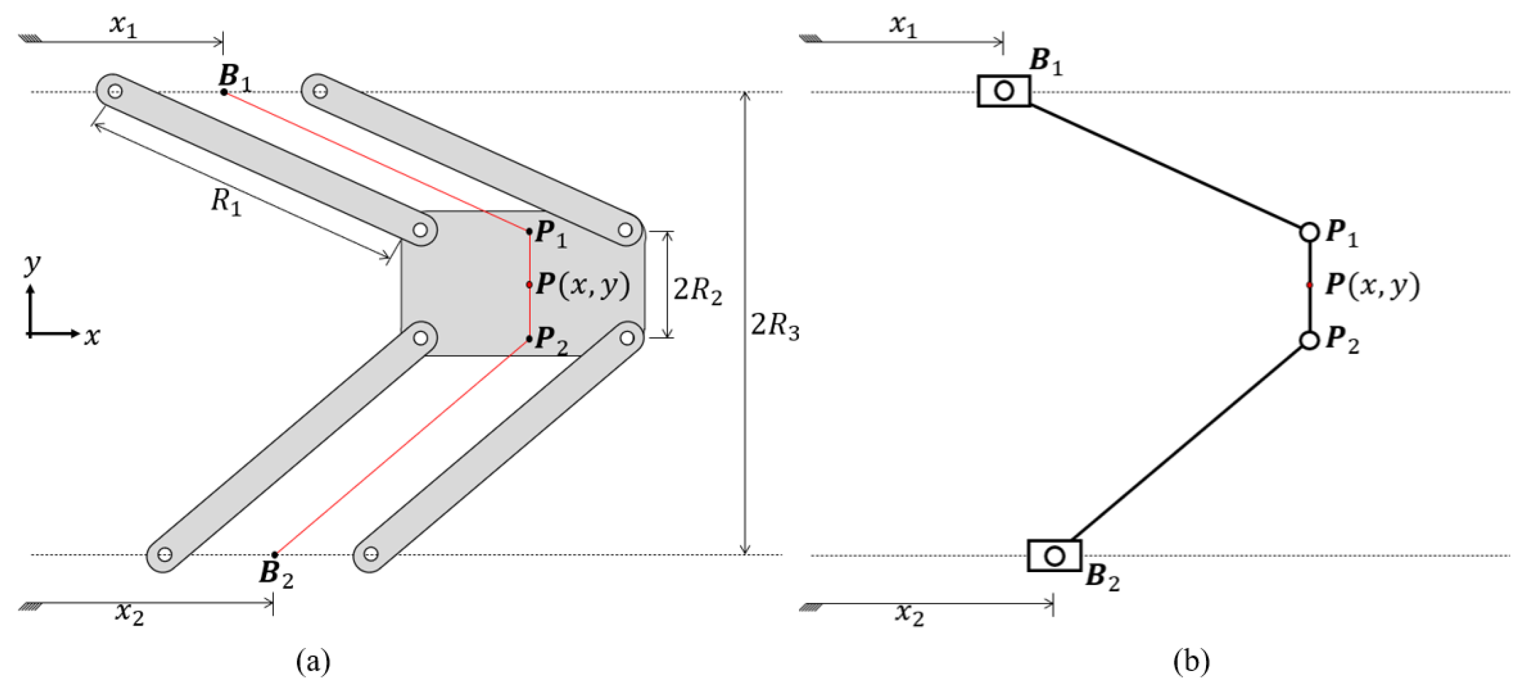
• Additionally, studies such as [5,16] do not present the considerations for machine design.

While this proposed system is still in silico, we will eventually conduct control design, manufacturing, experimental validation, and clinical trials.

2. Kinematic Model

The 2-PRR mechanism is driven by two linear actuators $\left({\mathbf{B}}_i\right)$, where the horizontal position of each actuator is denoted as $x_i$. The actuators cause the center point of a mobile platform $\left(\mathbf{P}\right)$ to move. Each end of the mobile platform is a binary joint $\left({\mathbf{P}}_i\right)$ that connects said platform to the actuators, $i=1,2$. The origin of our system, $\mathbf{0}={[0,0]}^T$, is positioned at the midpoint between both actuator rails. The distance between the actuator and platform edge is $R_1$, half of the height of the mobile platform is $R_2$, and the distance between any actuator rail and system origin is $R_3$. Parallelogram structures are formed, connected to each actuator, to prevent platform rotation, as seen in Figure 1a.

2.1. Inverse Kinematics

The position of each actuator ${\mathbf{B}}_i$ is a function of system geometry and the position of the mobile platform $(\mathbf{P}={[x,y]}^T)$. First, the position of point ${\mathbf{P}}_i$, $i=1,2$, in each platform binary link is calculated simply by moving up or down by a distance $R_2$:

$${\mathbf{P}}_1={[x,y+R_2]}^T,$$

(1)

$${\mathbf{P}}_2={[x,y-R_2]}^T.$$

(2)

The position of each actuator is

$${\mathbf{B}}_1={[x_1,R_3]}^T,$$

(3)

$${\mathbf{B}}_2={[x_2,-R_3]}^T.$$

(4)

The distance between ${\mathbf{P}}_i$ and ${\mathbf{B}}_i$ must be $R_1$, which is a geometric constraint of the mechanism

$$({\mathbf{P}}_i-{\mathbf{B}}_i)·{({\mathbf{P}}_i-{\mathbf{B}}_i)}^T=R_1^2;i=1,2.$$

(5)

Replacing x and y component values of Equations (1)–(4) in Equation (5) gives two scalar equations:

$${(x-x_1)}^2+{(y+R_2-R_3)}^2-R_1^2=0,$$

(6)

$${(x-x_2)}^2+{(y-R_2+R_3)}^2-R_1^2=0.$$

(7)

Solving Equation (6) for $x_1$ has a geometric equivalent to solving for the horizontal center position of a circumference of radius $R_1$ that passes through ${\mathbf{P}}_1$ at a center height of $R_3$, where there are two possible solutions. Solving for Equation (7) is analogous to Equation (6); then, four circumference centers are calculated. All permutations between the two superior and two lower circumference centers define a solution of the inverse geometric problem, resulting in four possible variations, as Figure 2a presents:

$$x_1=x\pm \sqrt{R_1^2-{(y+R_2-R_3)}^2},$$

(8)

$$x_2=x\pm \sqrt{R_1^2-{(y-R_2+R_3)}^2}.$$

(9)

The plus–minus sign of each solution represents an alternative way of assembling the mechanism, mirroring the horizontal position of the respective actuator with respect to a vertical line that passes through y. If an actuator is to the left of the mobile platform, as seen in Figure 1, the operation must be a subtraction.

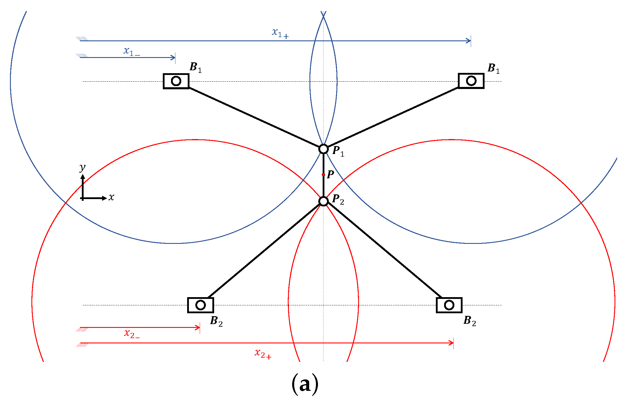
2.2. Forward Kinematics

The position $\mathbf{P}$ of the mobile platform is a function of system geometry and the positions of both actuators $(x_1,x_2)$. Equations (6) and (7) express the constraint of the mechanism. These equations form a non-linear system to solve for x and y. This non-linear system is geometrically equivalent to finding the intersection between two circumferences, whose centers $({{\mathbf{B}}_1}^{\prime },{{\mathbf{B}}_2}^{\prime })$ are separated by a horizontal distance of $2|R_3-R_2|$ and a height of $|x_1-x_2|$; therefore, there are two possible solutions, as Figure 2b presents:

$$\begin{array}{c}\hfill \mathbf{P}=\left[\begin{array}{c}{\displaystyle \frac{x_1+x_2}{2}}\pm {\displaystyle \frac{\left(R_2-R_3\right)}{2}}\sqrt{-{\displaystyle \frac{-4{R_1}^2+4{R_2}^2-8R_2{R}_3+4{R_3}^2+{x_1}^2-2x_1{x}_2+{x_2}^2}{{R_2}^2-2R_2{R}_3+{R_3}^2+4{x_1}^2-8x_1{x}_2+4{x_2}^2}}}\\ \\ \pm {\displaystyle \frac{1}{4}}\left(x_1-x_2\right)\sqrt{-{\displaystyle \frac{-4{R_1}^2+4{R_2}^2-8R_2{R}_3+4{R_3}^2+{x_1}^2-2x_1{x}_2+{x_2}^2}{{R_2}^2-2R_2{R}_3+{R_3}^2+4{x_1}^2-8x_1{x}_2+4{x_2}^2}}}\end{array}\right].\end{array}$$

(10)

Each solution is symmetrical to the line $\overline{{{\mathbf{B}}_1}^{\prime }{{\mathbf{B}}_2}^{\prime }}$.

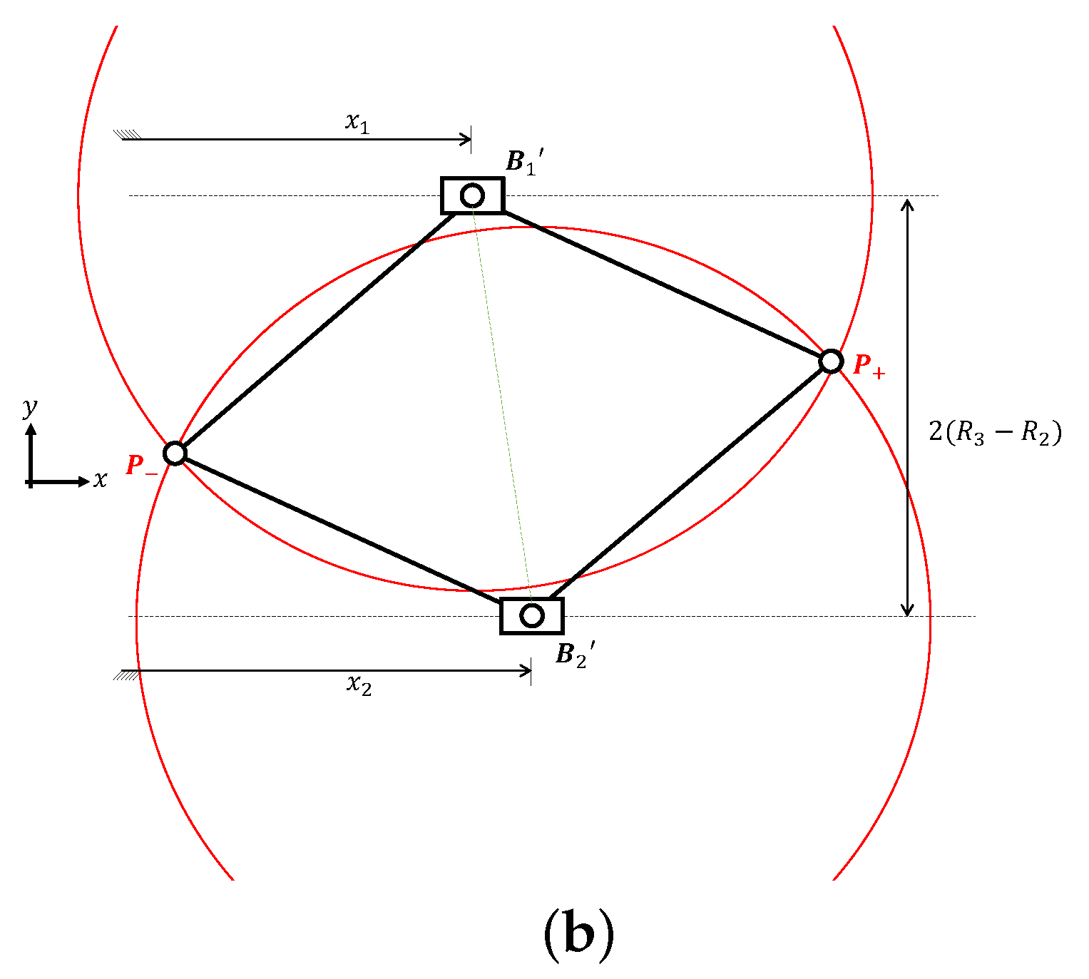
2.3. Singularity Analysis

Singularities can arise within the robot’s workspace. These singularities must be identified and avoided. In Section 2.1, we designated Equations (6) and (7) as a representation of geometric constraint; we will express this in a vector $\mathbf{F}$,

$$\mathbf{F}=\left[\begin{array}{c}{(x-x_1)}^2+{(y+R_2-R_3)}^2-R_1^2\\ {(x-x_2)}^2+{(y-R_2+R_3)}^2-R_1^2\end{array}\right].$$

(11)

If we express the input variables in a vector $\mathbf{q}={[x_1,x_2]}^T$ and the output variables in a vector $\mathbf{x}={[x,y]}^T$, we can identify singularities from the following differential model:

$$J_x\dot{\mathbf{x}}=J_q\dot{\mathbf{q}},$$

(12)

where $J_x$ is the Jacobian matrix of Equation (11) with respect to the output variables and $J_q$ is the negative Jacobian matrix of the same equation with respect to the input variables [30]. Evaluating the Jacobian matrix with respect to input variables,

$$J_q=-\frac{\partial \mathbf{F}}{\partial \mathbf{q}}=\left[\begin{array}{cc}2(x-x_1)& 0\\ 0& 2(x-x_2)\end{array}\right].$$

(13)

Evaluating the Jacobian matrix with respect to output variables,

$$J_x=\frac{\partial \mathbf{F}}{\partial \mathbf{x}}=\left[\begin{array}{cc}2(x-x_1)& 2(y+R_2-R_3)\\ 2(x-x_2)& 2(y-R_2+R_3)\end{array}\right].$$

(14)

For the determinant of the Jacobian matrix in Equation (13) to be zero,

$$\det \left(J_q\right)=(x-x_1)(x-x_2)=0,$$

$$x=x_1\mathrm{or}x=x_2.$$

(15)

Therefore, any position in which the mobile platform and an actuator are vertically aligned results in a singularity. The general Jacobian matrix of the 2-PRR is defined as $J={J_q}^{-1}{J}_x$,

$$\mathbf{J}=\left[\begin{array}{cc}1& {\displaystyle \frac{y+R_2-R_3}{x-x_1}}\\ 1& {\displaystyle \frac{y-R_2+R_3}{x-x_2}}\end{array}\right].$$

(16)

It is important to emphasize that this Jacobian represents a simplification of the true system that does not have the kinematic redundancy that two parallelogram linkages structures create. If only one parallelogram structure is considered, there will be functionality in the sense that the mobile platform will not be able to rotate; however, other singularities will arise. To avoid this, the kinematic redundancy is necessary when constructing the mechanism. We considered that all analyses performed with respect to this simplification will represent the system adequately. All performance indices were calculated taking into account these simplifications.

2.4. Parameter-Finiteness Normalization Method (PFNM)

Any number of synthesizable parameters $(R_i,i=1,2,3,\dots ,n)$ can have infinite possible values. The parameter-finiteness normalization method defines a finite design space that limits all mechanisms by means of a restraint relation that involves a normalization factor [28,31]. This process also results in one less parameter to take into account.

The dimensional synthesis of the 2-PRR mechanism consists of selecting three-dimensional parameters $(R_i,i=1,2,3)$. A normalization factor $\left(D\right)$ is defined as

$$D=\frac{R_1+R_2+R_3}{d},$$

(17)

where d is any positive number. Dividing each dimensional number by this normalization factor expresses three non-dimensional parameters $(r_i=R_i/D)$:

$$d=\frac{R_1+R_2+R_3}{D}=r_1+r_2+r_3.$$

(18)

In the case that $d=3$, we can express $r_3$ as

$$r_3=3-r_1-r_2,(0\le r_3\le 3).$$

(19)

Additionally, for assembly to be valid, $r_3<r_1+r_2$ and $r_2<r_1+r_3$, and this yields boundaries for our parameters; the geometric space where assembly conditions are satisfied is called the Parameter Design Space (PDS). The PDS for the 2-PRR mechanism is represented by a portion of an inclined plane. By using a transformation of variables, we can visualize the PDS as a function of two independent variables $(r_1,r_2,r_3⟶s,t)$,

$$s=\frac{2r_1+r_3}{\sqrt{3}},t=r_3.$$

(20)

This 2D PDS allows for the visualization of various kinematic performance indices using 2D surface plots (colormaps) as design atlases.

2.4.1. Non-Dimensional Translational Workspace Size

An index of particular interest is a relative workspace size. As a result of the nature of this mechanism, horizontal displacements are only delimited by the actuator position domain. Therefore, the workspace is bounded by half of the vertical capacity of the mobile platform. The non-dimensional translational workspace $\left(w_t\right)$ is, by definition, half of the vertical distance between singularity-inducing positions, as shown in Equation (15),

$$w_t=r_1-r_2+r_3,\mathrm{if}{r}_2>r_3$$

(21)

$$w_t=r_1+r_2-r_3,\mathrm{if}{r}_2<r_3.$$

(22)

Multiplying the normalization factor by the non-dimensional translational workspace results in the dimensional workspace length $\left(W_t\right)$:

$$W_t=w_t\left(D\right).$$

(23)

Biomechanical analyses allow for kinematic measurements of movements, e.g., employing motion capture systems based on the use of passive markers, infrared light, and force platforms to obtain more accurate and relevant data in studies of the movement of the human body [43]. In gait analysis, a kinematic analysis can determine movement characteristics such as the stride length and height, forces involved in the movement, and joint angles, which are measurements that serve as input parameters for the construction of systems that intervene with the gait pattern. The characteristics of the gait pattern can be affected by age, height, weight, and different pathologies. In older people, the speed and stride length decrease and depend on the height and weight of the person [44].

Reference [45] recognizes the human because of its variability as a product of biological and sociocultural evolution. The document presents studies of the anthropometric dimensions of some Latin American countries. Reference is made to Colombia, presenting data of dimensions in children, the working population between 20 and 59 years old, and the working population of the floricultural sector. Data were taken from this publication on the Colombian working population related to the lower body, accounting for the bias of age and sex, to define standard measures for a gait retraining device that adjusts to the Colombian population. Based on the percentages presented, it is possible to establish measures that will allow for the adjustment of the mechanical design for its correct functioning in the Colombian population.

Most of the articles in the literature refer to kinematic parameters measured from an absolute point of reference. However, it is sometimes helpful to analyze trajectories concerning a relative point of reference. In [46], a BWS treadmill gait retraining system called powered gait orthosis was designed by Shanghai University. In said paper, an analysis of hip displacement and ankle position was presented to show the relative ankle joint trajectory; the height of the ankle’s relative trajectory was approximately 15 cm. In [25,26], a similar trajectory was presented and the height of said trajectory was approximately 22 cm. Considering the design requirement for prior BWS systems and the anthropometric dimensions of the 95th percentile of the Colombian population, we established a design requirement for the gait retraining device to be able to trace a vertical distance of at least 25 cm.

The difference between the heights at the two singular points defined by Equation (15) $\left(\right|y\left(x_2\right)-y\left(x_1\right)\left|\right)$ represents the net vertical capacity of this mechanism. Therefore, this mechanism can move to any location as along as the height is within the interval,

$$\min (y\left(x_2\right),y\left(x_1\right))<y<\max (y\left(x_2\right),y\left(x_1\right)).$$

In practice, it is also best to avoid regions that are in close proximity with these limits. As a result, a tolerance of 20% was used to avoid singularity at these limits. Therefore, the actual workspace length was obtained by multiplying half of the vertical capacity by 1.20.

$$W_t=\frac{1.20(25 \mathrm{cm})}{2}=15\mathrm{cm}.$$

2.4.2. Minimum Linkage Length

If the non-dimensional translational workspace has been calculated and the true workspace length is known, the normalization factor can be calculated for every value of s and t $(D=W_t/w_t)$. Each value of s and t represents three values, $r_1,r_2,r_3$, that can be calculated by means of an anti-transform:

$$r_1=\frac{\sqrt{3}s-t}{2},r_2=3-\frac{\sqrt{3}s+t}{2},r_3=t.$$

(24)

The characteristic lengths of the 2-PRR mechanism $(R_1,2R_2,2R_3)$ are then calculated with the normalization factor to find the minimum characteristic length. With a known value of $W_t$ and the $w_t$ atlas, a minimum characteristic length atlas can be generated.

$$R_{\min }=\min \left[D\left(r_1\right),2D\left(r_2\right),2D\left(r_3\right)\right].$$

(25)

This way, the linkage size can be filtered to not be too small or too large. This is the only atlas that has dimensions and is specific to the design application.

2.4.3. Maximum and Global Conditioning Index

The condition number is a function of the mechanism Jacobian matrix and evaluates the accuracy of the control, the dexterity, and the isotropy of a mechanism. The minimum value that the condition number can have is one, which happens when the mechanism is in an isotropic pose. The inverse of the conditioning number is the local conditioning index. A global conditioning index must be calculated to evaluate the condition number of a mechanism over its workspace [30].

As a consequence, the local conditioning index must be integrated. As mentioned in Section 2.4.1, the workspace can be represented one-dimensionally. Therefore, the spatial integral over the workspace can be approximated as a sum of the local conditioning index along a line with N nodes:

$$GCI=\frac{{\displaystyle {\int }_W\left({\displaystyle \frac{1}{{\kappa }_j}}\right)\mathrm{d}W}}{{\displaystyle {\int }_W\mathrm{d}W}}={\displaystyle \frac{1}{N}}\sum _{n=1}^N{\left({\displaystyle \frac{1}{{\kappa }_j}}\right)}_n.$$

(26)

Another index to verify conditioning is the maximum local conditioning index of the mechanism; this is known as the maximum conditioning index $\left(MCI\right)$:

$$MCI=\max \left[{\left({\displaystyle \frac{1}{{\kappa }_j}}\right)}_n\right].$$

(27)

2.4.4. Global Rigidity Index

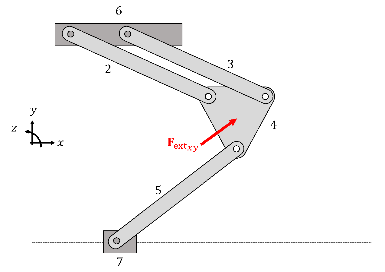
External forces can result in alterations in the position of the mobile platform: the less a mechanism displaces itself due to these external forces, the more rigid it is. The dimensions of the 2-PRR mechanism can also define the output mechanism displacement [47,48]:

$$\mathbf{D}=K^{-1}\mathit{\tau },$$

where K is called the mechanism stiffness matrix, $\mathit{\tau }$ is the external force vector, and $\mathbf{D}$ is the displacement vector. The stiffness vector is defined as

$$K=J^T\left[\begin{array}{cc}{k_p}_1& 0\\ 0& {k_p}_2\end{array}\right]J,$$

where ${k_p}_i$ represents the stiffness of each actuator. When ${k_p}_i=1$ and ${\left|\right|\mathit{\tau }\left|\right|}^2=1$, the magnitude of the maximum deformation can be calculated as the square root of the absolute maximum eigenvalue of the matrix ${\left(K^{-1}\right)}^T{K}^{-1}$:

$$\left|\right|{\mathbf{D}}_{\max }\left|\right|=\sqrt{\max \left(\right|{{\lambda }_D}_i\left|\right)},i=1,2.$$

The overall rigidity of the mechanism along the entire workspace can be calculated as the global stiffness index:

$$GSI=\frac{{\displaystyle {\int }_W\left|\right|{\mathbf{D}}_{\max }\left|\right|\mathrm{d}W}}{{\displaystyle {\int }_W\mathrm{d}W}}={\displaystyle \frac{1}{N}}\sum _{n=1}^N\left|\right|{\mathbf{D}}_{\max }{\left|\right|}_n.$$

(28)

3. Force Analysis

The 2-PRR mechanism presented in Figure 1a has a kinematic redundancy in the form of a second parallelogram structure, which is required to avoid singularities within the workspace. While this guarantees that the mobile platform will not rotate at any point, this also results in a statically indeterminate structure. A binary link replaces one of the parallelogram structures to estimate the reactions, as Figure 3 presents. The load that this new linkage will support will be greater than the shared load between the two linkages in the actual system. This worst-case scenario is used to design the 2-PRR mechanism.

In the context of our design, this mechanism will not be moving at high speeds compared to machinery designed for other industrial applications. Therefore, for any given mechanism pose, it was assumed that the inertial forces were not as significant as the effect of other external forces, thus resulting in a quasi-static model $(\sum \mathbf{F}\approx 0)$. Additionally, the weight of each linkage was negligible compared to the external force applied to the mechanism, which would be related to the weight of the user. For this reason, the mechanism weight was not included in the model. Since linkages 2, 3, and 5 are two-force members and the pose of each linkage is known using the kinematic model, the directions of all forces are known. This results in the following free-body-diagrams (FBDs), as shown in Figure 4.

Realizing the sum of forces and moments in the mobile platform, we can express one vectorial equation and one scalar equation:

$$\begin{array}{cc}\hfill {\mathbf{F}}_2+{\mathbf{F}}_3+{\mathbf{F}}_5+{\mathbf{F}}_{\mathrm{ext}}& =0,\hfill \end{array}$$

(29)

$$\begin{array}{cc}\hfill {\mathbf{r}}_2\times {\mathbf{F}}_2+{\mathbf{r}}_3\times {\mathbf{F}}_3+{\mathbf{r}}_5\times {\mathbf{F}}_5& =0.\hfill \end{array}$$

(30)

Separating horizontal and vertical force components results in three scalar equations:

$$\begin{array}{cc}\hfill F_{2}cos{\theta }_2+F_{3}cos{\theta }_2+F_{5}cos{\theta }_5& =-{F_{\mathrm{ext}}}_x,\hfill \\ \hfill F_{2}sin{\theta }_2+F_{3}sin{\theta }_2+F_{5}sin{\theta }_5& =-{F_{\mathrm{ext}}}_y,\hfill \\ \hfill F_2(-R_{2}sin{\theta }_2-R_{2}cos{\theta }_2)+F_3(R_2\sin {\theta }_2-R_2\cos {\theta }_2)+F_5(R_{2}cos{\theta }_5)& =0.\hfill \end{array}$$

Calling ${\alpha }_i=\cos {\theta }_i$, ${\beta }_i=\sin {\theta }_i$ and ${\gamma }_2=-R_{2}sin{\theta }_2-R_2\cos {\theta }_2)$, ${\gamma }_3=R_{2}sin{\theta }_2-R_{2}cos{\theta }_2$, ${\gamma }_5=R_{2}cos{\theta }_5$, the reaction forces can be calculated by solving the following linear system:

$$\left[\begin{array}{c}{F}_2\\ F_3\\ F_5\end{array}\right]={\left[\begin{array}{ccc}{\alpha }_2& {\alpha }_3& {\alpha }_5\\ {\beta }_2& {\beta }_3& {\beta }_5\\ {\gamma }_2& {\gamma }_3& {\gamma }_5\end{array}\right]}^{-1}\left[\begin{array}{c}-{F_{\mathrm{ext}}}_x\\ -{F_{\mathrm{ext}}}_y\\ 0\end{array}\right].$$

(31)

4. Machine Design

The cross-section selection for each link in the machine is solved using material strength criteria.

4.1. Static Failure

For links 2, 3, and 5, axial load $\left(F_i\right)$ will produce average normal stress of the form

$${\sigma }_{\mathrm{A}}=\frac{F_i}{A},$$

(32)

where A is the cross-section area. For linkage 4, the combination of all loads will produce an axial force, which will again produce normal stress and transversal loads that will produce bending moment and bending stress:

$${\sigma }_{\mathrm{B}}=\frac{M}{Z},$$

(33)

where Z is the cross-section modulus. Since the maximum static stress is a function of system geometry, said geometry can be varied until the ratio between the material strength and the maximum static stress bestows the safety factor. In the case of ductile materials, the material strength must be represented by the yield strength $\left(S_y\right)$ [49].

$$N_{\mathrm{static}}=\frac{S_y}{{\sigma }_{maxstatic}}.$$

(34)

4.2. Buckling Failure

Static stress alone is insufficient to determine the linkage safety when the axial load results in compressive loads. Each linkage in compression acts as a column that can buckle without warning if a critical load is surpassed [50,51]. The critical load of an intermediate column, also known as a Johnson column, is calculated as

$$\frac{P_{cr}}{A}=S_{yc}-\frac{1}{E}{\left(\frac{S_{yc}{S}_r}{2\pi }\right)}^2.$$

(35)

The critical load of slender columns, also known as Euler columns, can be expressed as

$$\frac{P_{cr}}{A}=E{\left(\frac{\pi }{S_r}\right)}^2.$$

(36)

Similar to static stress, the critical load is a function of the geometry and material properties. Therefore, system geometry is iterated until the ratio between the critical load and the maximum allowable operation load is above a selected safety factor.

$$N_{\mathrm{buckling}}=\frac{P_{cr}}{P_{\mathrm{allowable}}}.$$

(37)

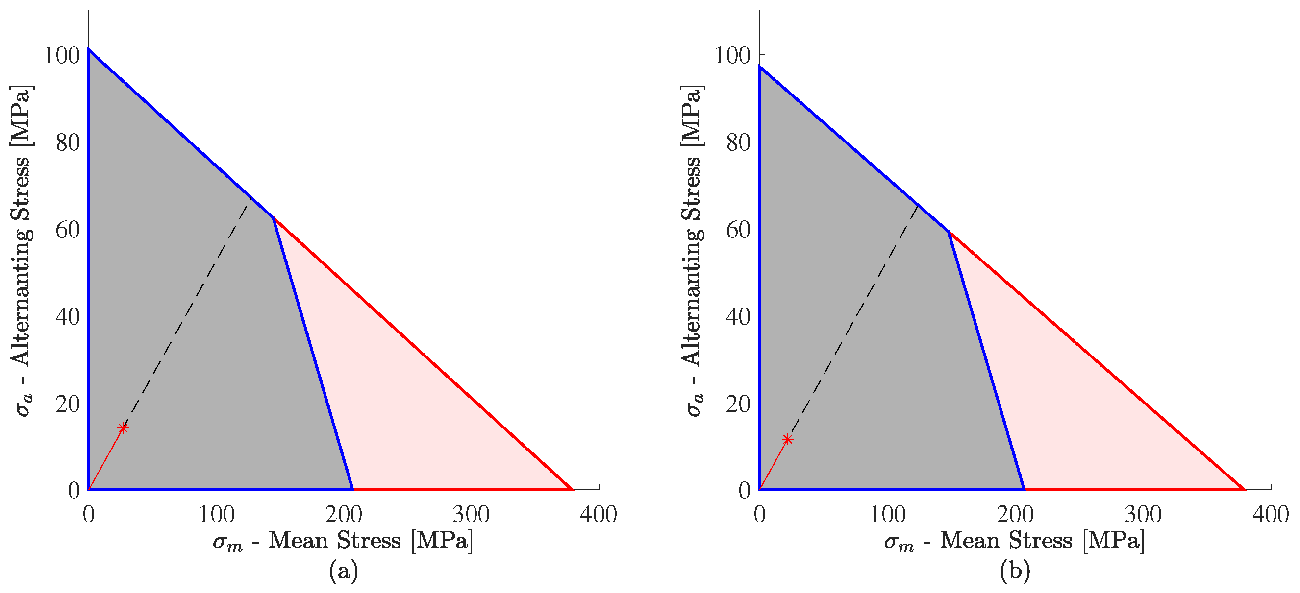
4.3. Fatigue Failure

Time-variable stress results in fatigue, and most machinery fails due to fatigue compared to static failure. In this context, the mechanism is considered a High-Cycle Fatigue (HCF) application designed by means of a stress-life approach according to the Goodman criteria [49,52].

5. Results

5.1. Performance Atlases

5.1.1. Non-Dimensional Workspace

Each point of the mechanism PDS was used to evaluate Equations (21) and (22). Evaluating the equations results in a 2D colormap, shown in Figure 5a. The southeast quadrant of the PDS represents adequate parallel manipulators.

5.1.2. Minimum Characteristic Length

Using Equation (25) with $W_t=15\mathrm{cm}$, the minimum characteristic length atlas was calculated. The largest dimensions tend to be a large number. All dimensions greater than 2 m were capped off at said limit to assist with the visualization of the design atlas; see Figure 5b.

5.1.3. Maximum and Global Conditioning Index

The conditioning indices were visualized, evaluating Equations (26) and (27). A higher index value represents more isotropy and controllability in the mechanism in both cases. Figure 5c and Figure 6a make it apparent that the $GCI$ atlas and $MCI$ atlas are similar. The most controllability can be found in the two dark-orange strips that originate from the northwest vertex.

5.1.4. Global Rigidity Index

The GSI can be visualized by evaluating Equation (28). The highest stiffness index tends to be a large number. All indices greater than seven were capped off at said limit to assist with the visualization of the design atlas. The most rigid mechanisms are found in the dark-blue regions near the northeast and southwest vertices of the PDS; see Figure 6b.

The regions with a higher stiffness index also appear to have a higher conditioning index, implying that optimizing a mechanism’s isotropy and rigidity will be relatively straightforward.

5.2. Dimensional Synthesis

Certain design restrictions were set in place to synthesize the 2-PRR mechanism.

$$\begin{array}{cc}\hfill & w_t\ge 0.5,\hfill \\ \hfill & R_{\min }\ge 15\mathrm{cm},\hfill \\ \hfill & GCI\ge 0.4,\hfill \\ \hfill & MCI\ge 0.7,\hfill \\ \hfill & GSI\le 2.0.\hfill \end{array}$$

Restrictions promote an adequate performance concerning size, isotropy, controllability, and rigidity. The PDS was then updated, eliminating all regions where said restrictions were not met; the region that satisfied the design restrictions $\left({\mathsf{\Omega }}_{w_t,GCI,MCI,GSI}\right)$ is shown in Figure 7.

The values $s=2.448$, $t=1.246$ were selected. This resulted in a normalization factor of $D=0.2988$ m and the dimensions: $R_1=44.72$ cm, $2R_2=15.33$ cm, $2R_3=74.47$ cm. Figure 8 presents a kinematic representation of the mechanism structure, the ankle trajectory developed by the mechanism end-effector, and a graphical representation of the user, all projected to the sagittal plane. The 2-PRR parallel robot and the user are represented by a kinematic diagram in which rotational pairs represent the user articulations, and the hip is assumed to be fixed to the ground link. The figure also presents the workspace and link parameters ($W_t$, $R_1$, $R_2$, $R_3$) obtained in the dimensional synthesis. Generalized coordinates are represented by $x_1$ and $x_2$ variables.

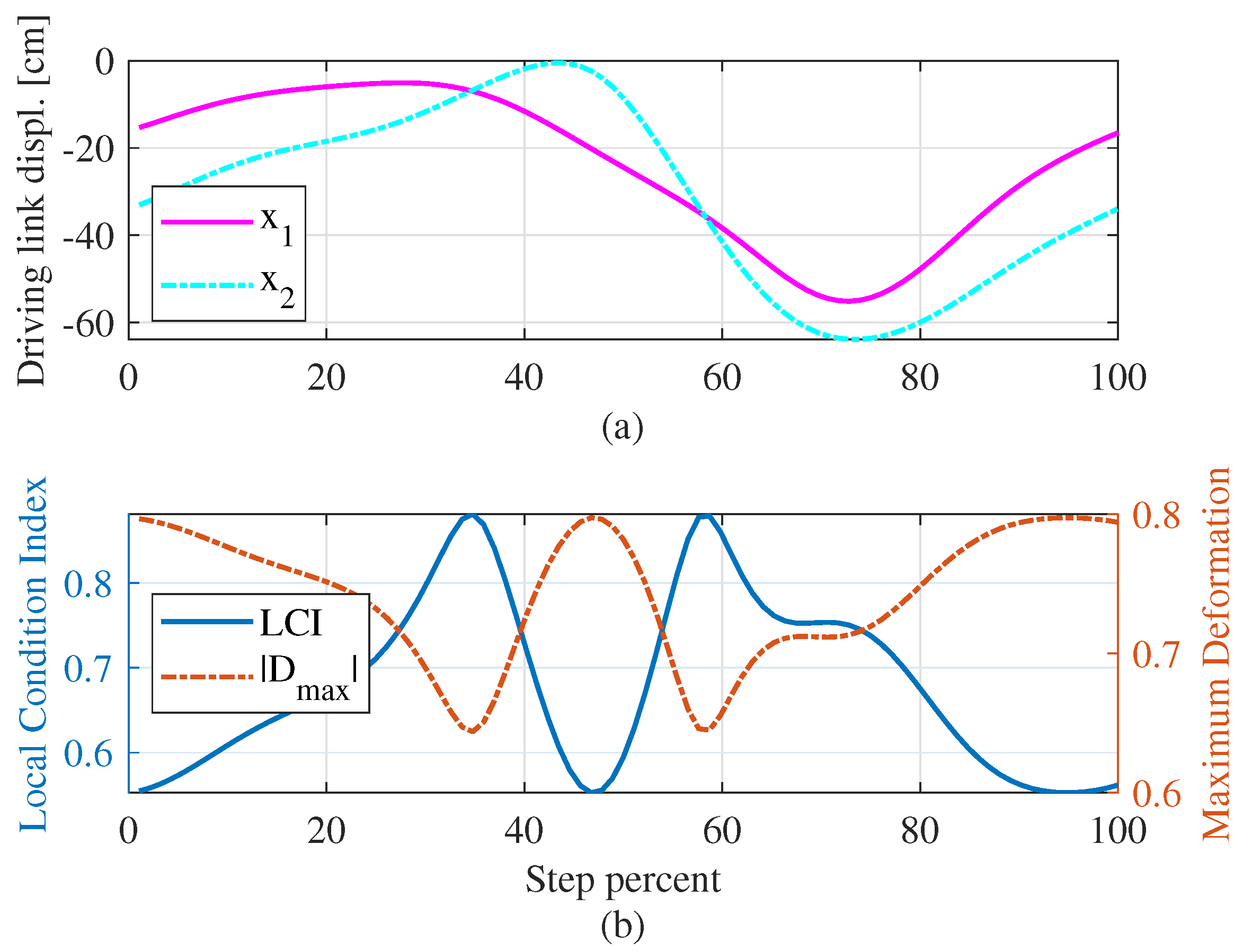
5.3. Validation of Kinematic Design Criteria

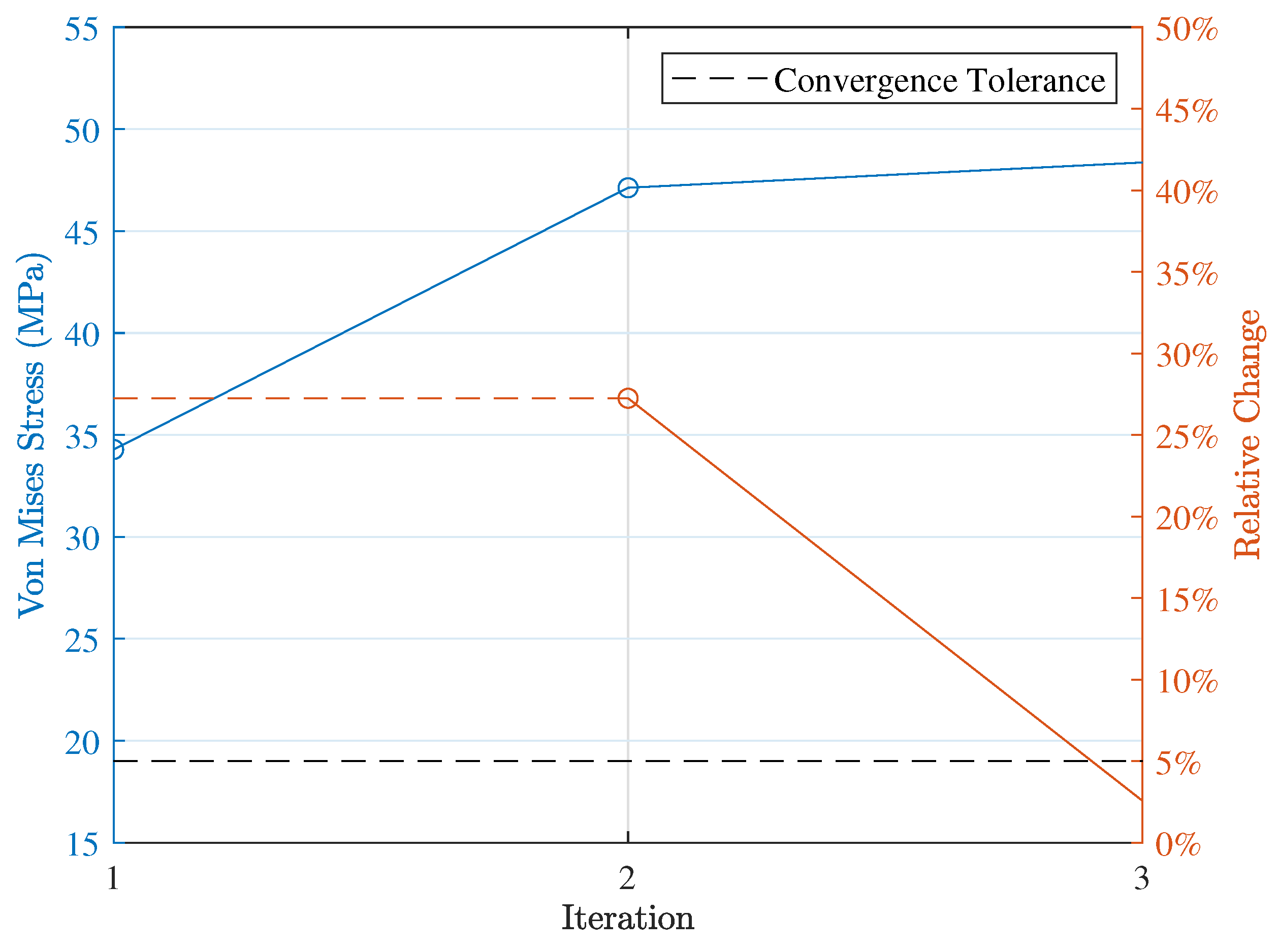
The type synthesis of the gait retraining mechanism was assessed by an interdisciplinary group using PCbDM, which results in the 2-PRR structure as described in the introduction. Two two-DoFs mechanisms were required to drive the limbs in the sagittal plane independently. The premise of driving the ankle in a programmable trajectory in the sagittal plane was assessed by performing a structural analysis (in the kinematic topology sense) of the linkage formed by one mechanism and the respective lower limb. The linkage structure was analyzed as a sequential assembly of determined and minimal kinematic chains (simple groups and Assur groups, as described by [54]). The chain is simple enough to determine the structure by inspection. However, algorithms such as [55,56,57] are available. The kinematic structure of the mechanism, which determines its kinematic behavior [58], is represented in Figure 9 in two ways: Figure 9a is a kinematic diagram that represents the geometric relations through kinematical pairs between the parallel robot (links 2 to 7), and the user’s limb (links 8 and 9), while Figure 9b is a structural graph in which each oval represents an independent kinematic chain, while the edges and layers represent the connections within the chains and the chain hierarchy. The hierarchy of the kinematic chains in Figure 9b is as follows: the first layer represents the two separate kinematic inputs, the second layer represents the kinematic chain that constrains the end-effector trajectory, and the third layer represents the user’s limb.

The kinematic performance $LCI$, $GCI$, $D_{max}$, and $GSI$ of the designed 2-PRR mechanism was assessed through a typical ankle trajectory, e.g., the trajectory in Figure 8. The results are compatible with design restrictions registered in the Dimensional Synthesis section, acknowledging that the analysis was restricted to the ankle’s trajectory. Figure 10 shows the performance of two local conditioning indexes through the ankle’s trajectory. Figure 10a presents the independent variables $x_1$ and $x_2$ as a function of the step percentage, while Figure 10b registers the corresponding $LCI$ and $D_{max}$. The accumulation of the local indexes through the trajectory results in the following global indexes: $GCI=0.682$, $MCI=0.881$, and $GSI=0.742$. The calculated local and global indexes verify, from a kinematic point of view, the mechanism’s controllability, dexterity, stiffness, and isotropy through a typical ankle trajectory, which likely promotes an adequate motion of a patient’s limb when implementing the gait retraining system.

5.4. Machine Design

Following Robert Norton’s guidelines, safety factors were determined, considering material property data, environmental conditions, and analytical models. Because the material property data are reasonably representative, environmental conditions correspond to room-ambience, and the analytical models accurately represent the system, the factors $(F_1=3,F_2=2,F_3=2)$ were selected. An additional factor of $ϵ=1.25$ was selected since this system has direct contact with humans [49]:

$$\begin{array}{cc}\hfill N_{min}& =ϵ\ast \max \left(F_i\right)\hfill \end{array}$$

(38)

$$\begin{array}{cc}\hfill & =1.25\ast 3=3.75.\hfill \end{array}$$

(39)

Therefore, all evaluated safety factors could not be inferior to $3.75$. Hollow cylinders allow for a sufficiently high rigidity and reduced weight for the linkage cross-section. Relative rotation between linkages was obtained using clevis joints. By threading the interior part of the cylinders, clevis joints with male threads could easily connect to each system. To facilitate manufacturing and possibly reduce overall costs, commercially available clevis joints with male threads were evaluated; specifically, joints based on the DIN 71751 standard [59]. There was a considerable stress concentration because of the sudden change in diameter between the linkages and the clevis joint male thread, which caused the clevis joint to support the most critical loads. Assuming a wall thickness of 4 mm for each linkage, the mechanism was modeled in CAD software and tested using a static-structural FEA simulation. The applied load was 1.2 kN on the center of the platform. The model assumed a linear elastic material, hot rolled SAE-AISI 1020 steel, with a yield strength of 207 MPa, 0.3 Poisson ratio, and 210 GPa Young’s Modulus. The number of elements in the mesh was refined adaptively until the convergence of a baseline variable was obtained (h-refinement). In this case, the baseline variable to evaluate convergence was Von Mises stress and the convergence tolerance was 5%. The mesh consisted of 10 node 3D tetrahedral elements with a maximum element size of 5% of the model size and a maximum aspect ratio of 10. Convergence occurs within three increments, with a final mesh of 35,750 elements and 69,805 nodes. Displacement-related failure was not a factor due to the infinitesimal displacements caused by the loads; the maximum nodal displacement was 93.47 µm. The change in Von Mises stress for the M16 geometry is shown in Figure 11. The only clevis joints that gave valid safety factors according to the static stress studies were the M16 and the M20 clevis joints, with safety factors of 4.28 and 20.08, respectively.

A buckling model was realized for a general tube of interior diameter d and external diameter D, as described in Section 4.2. Each cross-section was characterized as either a Johnson or a Euler column, and the safety factor was computed using Equation (37); to evaluate that equation we assumed a compressive yield strength of 207 MPa for hot rolled SAE-AISI 1020 steel. This can be visualized as a 3D surface (safety factor as a function of d and D) or a 2D colormap, as shown in Figure 12. The regions where $d>D$ represent invalid geometries are highlighted in red and the region where the minimum safety is met is highlighted as a magenta line.

To be able to couple the M16 or M20 clevis threads, the interior diameter of the linkages must be either 16 mm or 20 mm; the assumption of a 4 mm wall thickness causes the exterior diameter to be either 20 mm or 24 mm $(d=16\mathrm{mm}, D=20\mathrm{mm}\mathrm{or}d=20\mathrm{mm},$$D=24\mathrm{mm})$. Each of these points results in a safety factor of 13.20 (M16) or 16.91 (M20).

Finally, a stress-life model was evaluated, as described in Section 4.3, for both available geometries. After calculating the load, size, surface, temperature, corrosion, and reliability factors, the endurance limit was 100.96 MPa (M16) and 97.14 MPa (M20). The maximum and minimum loads were used to find the mean and alternating stress from the quasi-static model. With this information, the Goodman diagrams were constructed, as seen in Figure 13.

For each case, the loading case is clear of fatigue failure. The safety factors were 4.74 (M16) and 5.64 (M20), and there is no risk of plastic deformations (red region of Goodman diagram). Since both geometries present valid safety factors for static stress, buckling failure, and fatigue failure, the cross-section with the minor area is preferred; this results in less volume and ultimately less mass, which resulted in the M16 clevis being an adequate choice for the system.

6. Discussion

A two-DoFs parallel manipulator was designed to serve as the end-effector of a gait retraining system. The dimensional synthesis included workspace, isotropy, stiffness, and size constraints to obtain a valid point in the 2D parameter design space. This point represents three characteristic dimensions. The cross-section geometry was based on clevis joints with male threads. Analytical models were constructed to be able to design each linkage to be able to resist buckling and fatigue failure; see Figure 14a. Static stress safety was obtained by means of an FEA model. The geometry of the central platform was based on a DIN 71751 clevis tang; see Figure 14b.

To be able to coordinate the mechanism, two actuators must be controlled; this could be generated multiple ways. For example, two power-screws can be turned by two motors to advance a bolt-like adapter that will make the parallelogram linkage advance or retreat, as seen in Figure 14c.

While this investigation was still in silico, we expect that, with a proper control system, two of these mechanisms will be able to move a patient’s ankle and induce specific motor coordination exercises that can activate certain muscle groups and encourage neural plasticity to help retrain his or her gait. Significant evidence of the end-effector gait retraining system performance supports this hypothesis. Two studies on the G-EO system (an end-effector gait retraining system based on a parallel robot) report the superior rehabilitation performance of subacute stroke and central nervous system lesion patients compared to physiotherapy and physiotherapy-plus-treadmill rehabilitation [13,60]. Regarding the 2-PRR end-effector gait retraining system, the external evidence allows us to expect a safe, trustworthy, simple, and more affordable gait retraining system than those currently available in Colombia. The 2-PRR gait retraining system can be seen with a patient’s lower limbs to scale in Figure 15.

Some drawbacks of this system are: the system can coordinate the relative kinematics of the knee and ankle regarding the hip. However, there is no control over the movement of any part of the foot below the ankle. Additionally, peripheral components still need to be designed for a complete functioning gait retraining system, and these components include limiting the movement of the knee and hip to the sagittal plane and supporting the patient’s body weight.

References

1. Sale, P.; Franceschini, M.; Waldner, A.; Hesse, S. Use of the robot assisted gait therapy in rehabilitation of patients with stroke and spinal cord injury. Eur. J. Phys. Rehabil. Med. 2012, 48, 21–111. [Google Scholar]
2. Calabrò, R.; Cacciola, A.; Bertè, F.; Manuli, A.; Leo, A.; Bramanti, A.; Naro, A.; Milardi, D.; Bramanti, P. Robotic gait rehabilitation and substitution devices in neurological disorders: Where are we now? Neurol. Sci. 2016, 37, 503–514. [Google Scholar] [CrossRef] [PubMed]
3. Hobbs, B.; Artemiadis, P. A Review of robot-assisted lower-limb Stroke therapy: Unexplored paths and future directions in gait rehabilitation. Front. Neurorobot. 2020, 14, 19. [Google Scholar] [CrossRef] [Green Version]
4. Kapsalyamov, A.; Jamwal, P.; Hussain, S.; Ghayesh, M. State of the art lower limb robotic exoskeletons for elderly assistance. IEEE Access 2019, 7, 95075–95086. [Google Scholar] [CrossRef]
5. Jezernik, S.; Colombo, G.; Keller, T.; Frueh, H.; Morari, M. Robotic orthosis Lokomat: A rehabilitation and research tool. Neuromodul. Technol. Neural Interface 2003, 6, 108–115. [Google Scholar] [CrossRef] [PubMed]
6. Veneman, J.; Kruidhof, R.; Hekman, E.; Ekkelenkamp, R.; Van Asseldonk, E.; Van Der Kooij, H. Design and evaluation of the LOPES exoskeleton robot for interactive gait rehabilitation. IEEE Trans. Neural Syst. Rehabil. Eng. 2007, 15, 379–386. [Google Scholar] [CrossRef] [PubMed] [Green Version]
7. Zoss, A.; Kazerooni, H.; Chu, A. Biomechanical design of the Berkeley lower extremity exoskeleton (BLEEX). IEEE/ASME Trans. Mechatron. 2006, 11, 128–138. [Google Scholar] [CrossRef]
8. Wang, S.; Zhang, B.; Yu, Z.; Yan, Y. Differential soft sensor-based measurement of interactive force and assistive torque for a robotic hip exoskeleton. Sensors 2021, 21, 6545. [Google Scholar] [CrossRef]
9. Kennard, M.; Kadone, H.; Shimizu, Y.; Suzuki, K. Passive exoskeleton with gait-based knee joint support for individuals with cerebral palsy. Sensors 2022, 22, 8935. [Google Scholar] [CrossRef]
10. Narayan, J.; Dwivedy, S.K. Preliminary design and development of a low-cost lower-limb exoskeleton system for paediatric rehabilitation. Proc. Inst. Mech. Eng. Part H 2021, 235, 530–545. [Google Scholar] [CrossRef]
11. Sunilkumar, P.; Mohan, S.; Mohanta, J.K.; Wenger, P.; Rybak, L. Design and motion control scheme of a new stationary trainer to perform lower limb rehabilitation therapies on hip and knee joints. Int. J. Adv. Robot. Syst. 2022, 19, 17298814221075184. [Google Scholar] [CrossRef]
12. Glowinski, S.; Ptak, M. A kinematic model of a humanoid lower limb exoskeleton with pneumatic actuators. Acta Bioeng. Biomech. 2022, 24, 145–157. [Google Scholar] [CrossRef]
13. Hesse, S.; Schattat, N.; Mehrholz, J.; Werner, C. Evidence of end-effector based gait machines in gait rehabilitation after CNS lesion. NeuroRehabilitation 2013, 33, 77–84. [Google Scholar] [CrossRef] [PubMed]
14. Hesse, S.; Sarkodie-Gyan, T.; Uhlenbrock, D. Development of an advanced mechanised gait trainer, controlling movement of the centre of mass, for restoring gait in non-ambulant subjects—Weiterentwicklung eines mechanisierten gangtrainers mit steuerung des massenschwerpunktes zur gangrehabilitation rollstuhlpflichtiger patienten. Biomed. Tech. Eng. 1999, 44, 194–201. [Google Scholar] [CrossRef]
15. Schmidt, H.; Sorowka, D.; Hesse, S.; Bernhardt, R. Entwicklung eines robotergestützten laufsimulators zur gangrehabilitation. Development of a robotic walking simulator for gait rehabilitation. Biomed. Tech. Eng. 2003, 48, 281–286. [Google Scholar] [CrossRef]
16. Hesse, S.; Waldner, A.; Tomelleri, C. Innovative gait robot for the repetitive practice of floor walking and stair climbing up and down in stroke patients. J. NeuroEng. Rehabil. 2010, 7, 30. [Google Scholar] [CrossRef] [Green Version]
17. Bruni, M.F.; Melegari, C.; De Cola, M.C.; Bramanti, A.; Bramanti, P.; Calabrò, R.S. What does best evidence tell us about robotic gait rehabilitation in stroke patients: A systematic review and meta-analysis. J. Clin. Neurosci. 2018, 48, 11–17. [Google Scholar] [CrossRef]
18. Awad, L.; Bae, J.; O’Donnell, K.; De Rossi, S.M.M.; Hendron, K.; Sloot, L.H.; Kudzia, P.; Allen, S.; Holt, K.G.; Ellis, T.D.; et al. A soft robotic exosuit improves walking in patients after stroke. Sci. Transl. Med. 2017, 9, eaai9084. [Google Scholar] [CrossRef] [Green Version]
19. Lee, S.H.; Park, G.; Cho, D.Y.; Kim, H.Y.; Lee, J.; Kim, S.; Park, S.B.; Shin, J.H. Comparisons between end-effector and exoskeleton rehabilitation robots regarding upper extremity function among chronic stroke patients with moderate-to-severe upper limb impairment. Sci. Rep. 2020, 10, 1806. [Google Scholar] [CrossRef] [Green Version]
20. Li, W.Z.; Cao, G.Z.; Zhu, A.B. Review on control strategies for lower limb rehabilitation exoskeletons. IEEE Access 2021, 9, 123040–123060. [Google Scholar] [CrossRef]
21. Dollar, A.M.; Herr, H. Lower extremity exoskeletons and active orthoses: Challenges and state-of-the-art. IEEE Trans. Robot. 2008, 24, 144–158. [Google Scholar] [CrossRef]
22. Hamza, M.F.; Ghazilla, R.A.R.; Muhammad, B.B.; Yap, H.J. Balance and stability issues in lower extremity exoskeletons: A systematic review. Biocybern. Biomed. Eng. 2020, 40, 1666–1679. [Google Scholar] [CrossRef]
23. O’Sullivan, L.; Nugent, R.; van der Vorm, J. Standards for the safety of exoskeletons used by industrial workers performing manual handling activities: A contribution from the Robo-Mate Project to their future development. Procedia Manuf. 2015, 3, 1418–1425. [Google Scholar] [CrossRef] [Green Version]
24. Collo, A.; Bonnet, V.; Venture, G. A quasi-passive lower limb exoskeleton for partial body weight support. In Proceedings of the 6th IEEE International Conference on Biomedical Robotics and Biomechatronics (BioRob), Singapore, 26–29 June 2016. [Google Scholar] [CrossRef]
25. Tsuge, B.; Mccarthy, J. Synthesis of a 10-Bar linkage to guide the gait cycle of the human leg. In Proceedings of the 39th Mechanisms and Robotics Conference, Boston, MA, USA, 2–5 August 2015. [Google Scholar] [CrossRef] [Green Version]
26. Tsuge, B.; Mccarthy, J. An adjustable single degree-of-freedom system to guide natural walking movement for rehabilitation. J. Med. Devices. 2016, 10, 44501. [Google Scholar] [CrossRef] [Green Version]
27. Shao, Y.; Xiang, Z.; Liu, H.; Li, L. Conceptual design and dimensional synthesis of cam-linkage mechanisms for gait rehabilitation. Mech. Mach. Theory 2016, 104, 31–42. [Google Scholar] [CrossRef]
28. Liu, X.J.; Wang, J.; Pritschow, G. Kinematics, singularity and workspace of planar 5R symmetrical parallel mechanisms. Mech. Mach. Theory 2006, 41, 145–169. [Google Scholar] [CrossRef]
29. Merlet, J.P.; Daney, D. Appropriate design of parallel manipulators. In Smart Devices and Machines for Advanced Manufacturing; Springer: London, UK, 2008; pp. 1–25. [Google Scholar] [CrossRef] [Green Version]
30. Merlet, J.P. Jacobian, manipulability, condition number, and accuracy of parallel robots. J. Mech. Des. 2005, 128, 199–206. [Google Scholar] [CrossRef]
31. Liu, X.J.; Wang, J. A new methodology for optimal kinematic design of parallel mechanisms. Mech. Mach. Theory 2007, 42, 1210–1224. [Google Scholar] [CrossRef]
32. Mohan, S.; Mohanta, J.; Kurtenbach, S.; Paris, J.; Corves, B.; Huesing, M. Design, development and control of a 2PRP-2PPR planar parallel manipulator for lower limb rehabilitation therapies. Mech. Mach. Theory 2017, 112, 272–294. [Google Scholar] [CrossRef]
33. Mohanta, J.; Mohan, S.; Deepasundar, P.; Kiruba-Shankar, R. Development and control of a new sitting-type lower limb rehabilitation robot. Comput. Electr. Eng. 2018, 67, 330–347. [Google Scholar] [CrossRef]
34. Vasanthakumar, M.; Vinod, B.; Mohanta, J.K.; Mohan, S. Design and robust motion control of a planar 1P-2P RP hybrid manipulator for lower limb rehabilitation applications. J. Intell. Robot. Syst. 2019, 96, 17–30. [Google Scholar] [CrossRef]
35. Baker, R. Measure Walking: A Handbook of Clinical Gait Analysis; Mac Keith Press: London, UK, 2013. [Google Scholar]
36. Cross, N. Engineering Design Methods: Strategies for Product Design, 5th ed.; John Wiley & Sons Ltd.: Hoboken, NJ, USA, 2021; ISBN 0-13-612370-8. [Google Scholar]
37. Molteni, F.; Gasperini, G.; Cannaviello, G.; Guanziroli, E. Exoskeleton and end-effector robots for upper and lower limbs rehabilitation: Narrative review. PM&R. 2018, 10, 174–188. [Google Scholar] [CrossRef] [Green Version]
38. Mehrholz, J.; Pohl, M.; Platz, T.; Kugler, J.; Elsner, B. Electromechanical and robot-assisted arm training for improving activities of daily living, arm function, and arm muscle strength after stroke. Cochrane Database Syst. Rev. 2015, 9, CD006876. [Google Scholar] [CrossRef] [PubMed]
39. Chen, B.; Lanotte, F.; Grazi, L.; Vitiello, N.; Crea, S. Classification of lifting techniques for application of a robotic hip exoskeleton. Sensors 2019, 19, 963. [Google Scholar] [CrossRef] [Green Version]
40. Chen, B.; Zi, B.; Qin, L.; Pan, Q. State-of-the-art research in robotic hip exoskeletons: A general review. J. Orthop. Transl. 2020, 20, 4–13. [Google Scholar] [CrossRef]
41. Barragán, J.; Ovalle, G. Entrenador de Marcha Para el Ejercicio de Miembros Inferiores Humanos. Colombian Patent Resolución No 202194, 29 April 2020. [Google Scholar]
42. Manchola, M.; Serrano, D.; Gómez, D.; Ballen, F.; Casas, D.; Munera, M.; Cifuentes, C. T-FLEX: Variable stiffness ankle-foot orthosis for gait assistance. In Wearable Robotics: Challenges and Trends. WeRob 2018; Carrozza, M., Micera, S., Pons, J., Eds.; Biosystems & Biorobotics; Springer: Cham, Switzerland, 2019; Volume 22. [Google Scholar] [CrossRef]
43. Prakash, C.; Gupta, K.; Mittal, M.; Kumar, R.; Laxmi, V. Passive marker based optical system for gait Kinematics for lower extremity. Procedia Comput. Sci. 2015, 45, 176–185. [Google Scholar] [CrossRef] [Green Version]
44. Samson, M.; Crowe, A.; de Vreede, P.; Dessens, J.; Duursma, S.; Verhaar, H. Differences in gait parameters at a preferred walking speed in healthy subjects due to age, height and body weight. Aging Clin. Exp. Res. 2001, 13, 16–21. [Google Scholar] [CrossRef]
45. Avila-Chaurand, R.; Prado-León, L.; González-Muñoz, E. Dimensiones Antropométricas de la Población Latinoamericana: México, Cuba, Colombia, Chile; Universidad de Guadalajara: Jalisco, Mexico, 2007. [Google Scholar]
46. Wang, Q.; Qian, J.; Zhang, Y.; Shen, L.; Zhang, Z.; Feng, Z. Gait trajectory planning and simulation for the powered gait orthosis. In Proceedings of the 2007 IEEE International Conference on Robotics and Biomimetics (ROBIO), Sanya, China, 15–18 December 2007; pp. 1693–1697. [Google Scholar] [CrossRef]
47. Liu, X.J.; Wang, J.; Pritschow, G. Performance atlases and optimum design of planar 5R symmetrical parallel mechanisms. Mech. Mach. Theory 2006, 41, 119–144. [Google Scholar] [CrossRef]
48. Liu, X.J.; Wang, J. A new index for the performance evaluation of parallel manipulators: A study on planar parallel manipulators. In Proceedings of the 2008 7th World Congress on Intelligent Control and Automation, Chongqing, China, 25–27 June 2008; Volume 42. [Google Scholar] [CrossRef]
49. Norton, R. Machine Design: An Integrated Approach, 4th ed.; Prentice Hall: Hoboken, NJ, USA, 2010; ISBN 0-13-612370-8. [Google Scholar]
50. Nisbeth, J.; Budyna, R. Shigley’s Mechanical Engineering Design; McGraw-Hill Education: Columbus, OH, USA, 2019. [Google Scholar]
51. Aziz, H.; Al-alkawi, H. An appraisal of Euler and Johnson buckling theories under dynamic compression buckling loading. Iraqi J. Mech. Mater. Eng. 2009, 9, 173–181. Available online: https://www.iasj.net/iasj/article/63758 (accessed on 15 November 2021).
52. Lee, Y.L.; Pan, J.; Hathaway, R.; Barkey, M. Fatigue Testing and Analysis: Theory and Practice; Elsevier Science & Technology: Amsterdam, The Netherlands, 2016. [Google Scholar]
53. Durango, S.; Delgado, M.C.; Álvarez, C.; Flórez, R.; Flórez, M. Kinematic design of a 2-PRR parallel robot. Sci. Tech. 2020, 25, 372–379. [Google Scholar] [CrossRef]
54. Kolovsky, M.; Evgrafov, A.; Semenov, Y.; Slousch, A. Geometric analysis of mechanisms. In Advanced Theory of Mechanisms and Machines; Springer: Berlin/Heidelberg, Germany, 2000; pp. 41–78. [Google Scholar]
55. Saura, M.; Celdran, A.; Dopico, D.; Cuadrado, J. Computational structural analysis of planar multibody systems with lower and higher kinematic pairs. Mech. Mach. Theory 2014, 71, 79–92. [Google Scholar] [CrossRef]
56. Sun, Y.; Ge, W.; Zheng, J.; Dong, D. Solving the kinematics of the planar mechanism using data structures of Assur groups. J. Mech. Robot. 2016, 8, 061002-13. [Google Scholar] [CrossRef]
57. Durango, S.; Correa, J.; Ruiz, O. Graph-based structural analysis of planar mechanisms. Meccanica 2017, 52, 441–455. [Google Scholar] [CrossRef]
58. Müller, A. Representation of the kinematic topology of mechanisms for kinematic analysis. Mech. Sci. 2015, 6, 137–146. [Google Scholar] [CrossRef]
59. DIN Standard 71751; [Fork Joints—Synopsis]. Deutsches Institut für Normung: Berlin, Germany, 1975.
60. Hesse, S.; Tomelleri, C.; Bardeleben, A.; Werner, C.; Waldner, A. Robot-assisted practice of gait and stair climbing in nonambulatory stroke patients. J. Rehabil. Res. Dev. 2012, 49, 613–622. [Google Scholar] [CrossRef] [PubMed]
Figure 1. 2-PRR parallel mechanism: (a) general representation; (b) equivalent kinematic diagram.
Machines 11 00788 g001
Figure 2. Representation of (a) four possible solutions for the inverse kinematic geometric problem and (b) two possible solutions for the forward kinematic geometric problem.
Machines 11 00788 g002aMachines 11 00788 g002b
Figure 3. 2-PRR parallel mechanism representation for force analysis.
Machines 11 00788 g003
Figure 4. Simplified FBDs, expressing linkages 2, 3, and 5 as two force members.
Machines 11 00788 g004
Figure 5. Design atlases for (a) ( w t ) , (b) R min , and (c) G C I . (a,c) from [53] (License: CC-BY-NC-ND 4.0). (b) is the only dimensional atlas presented in this work, and is only valid for W t = 15 cm .
Machines 11 00788 g005aMachines 11 00788 g005b
Figure 6. Design atlases (continued) for (a) M C I and (b) G S I . (a) from [53] (License: CC-BY-NC-ND 4.0).
Machines 11 00788 g006
Figure 7. Updated PDS that represents synthesizable 2-PRR mechanisms that satisfy design restrictions.
Machines 11 00788 g007
Figure 8. Sketch of 2-PRR mechanism, typical ankle trajectory, and user. Movement is registered relative to the hip. 2 W t = 30 cm, R 1 = 44.72 cm, 2 R 2 = 15.33 cm, 2 R 3 = 74.47 cm.
Machines 11 00788 g008
Figure 9. Gait retraining system linkage. (a) Kinematic diagram. (b) Structural graph. Ovals: the first number is the number of links forming the group, the second is the DoFs regarding other groups forming pairs, and the superscript is the identification of links forming the group. Arrows register the connection between groups and the generation sequence.
Machines 11 00788 g009
Figure 10. Kinematic performance of 2-PRR mechanism. (a) Displacement of driving links required to achieve ankle’s trajectory in Figure 8. (b) L C I (solid line) and D m a x (dashed line) calculated through ankle’s trajectory in Figure 8. The G C I , M C I , and G S I calculated over L C I and D m a x are G C I = 0.682 , M C I = 0.881 , and G S I = 0.742 .
Machines 11 00788 g010
Figure 11. Convergence of Von Mises stress.
Machines 11 00788 g011
Figure 12. Buckling safety factor for a general tube of interior diameter d and external diameter D.
Machines 11 00788 g012
Figure 13. Goodman diagram for (a) M16 and (b) M20 clevis geometry.
Machines 11 00788 g013
Figure 14. CAD model of a 2-PRR parallel robot designed for gait retraining. (a) General view. (b) Mobile platform with clevis-tang-like geometry. (c) Power-screw actuated parallelogram.
Machines 11 00788 g014
Figure 15. CAD geometric model of a gait retraining system based on two 2-PRR parallel robots. (a) Side view. (b) Isometric view.
Machines 11 00788 g015