Supply Chain 4.0: A Machine Learning-Based Bayesian-Optimized LightGBM Model for Predicting Supply Chain Risk

Abstract

In today’s intricate and dynamic world, Supply Chain Management (SCM) is encountering escalating difficulties in relation to aspects such as disruptions, globalisation and complexity, and demand volatility. Consequently, companies are turning to data-driven technologies such as machine learning to overcome these challenges. Traditional approaches to SCM lack the ability to predict risks accurately due to their computational complexity. In the present research, a hybrid Bayesian-optimized Light Gradient-Boosting Machine (LightGBM) model, which accurately forecasts backorder risk within SCM, has been developed. The methodology employed encompasses the creation of a mathematical classification model and utilises diverse machine learning algorithms to predict the risks associated with backorders in a supply chain. The proposed LightGBM model outperforms other methods and offers computational efficiency, making it a valuable tool for risk prediction in supply chain management.

1. Introduction

In the era of Industry 4.0, businesses are increasingly relying on advanced technologies and data-driven approaches to optimise their supply chain processes. Supply chain risk management (SCRM) has emerged as a critical area of focus, as disruptions in this area can significantly impact the overall performance and profitability of organisations [1]. Past events like the tsunamis in 2004 and 2011, hurricane Katrina in the US in 2005, the volcanic eruption in Iceland in 2010, and the ongoing COVID-19 pandemic demonstrate how networks and entire industries can be negatively impacted [2,3]. Therefore, risk management in the industry and supply chains has become increasingly important due to the complex relationships between different chain components. Unlike when mass production required fewer components, today’s supply chains involve more stakeholders (suppliers, customers, regulators, and competitors), making them more vulnerable to disruptions and malfunctions [4]. To prevent and mitigate disturbances, disruptive innovations like digitalisation and Industry 4.0 have driven the development of new paradigms in SCRM, leveraging big data analytics, the Internet of Things (IoT), blockchain, and advanced deep learning (ADL) to help predict future trends and make informed decisions in supply chain management (SCM) [2,5,6]. Researchers and practitioners have turned to machine learning techniques for predictive analytics to mitigate and address these risks effectively [7,8]. This paper explores the application of a Machine Learning-based Bayesian-optimized Light Gradient-Boosting Machine (LightGBM) model for predicting supply chain back-order risk, enabling improved visibility, agility, and responsiveness. Supply chain backorder risk refers to the likelihood and impact of facing stockouts or unfulfilled customer orders due to inventory shortages or disruptions in a supply chain [9], while machine learning can broadly be defined as an algorithm that generates outputs based on available data without first programming the respective learning outcome [10]. Bayesian optimisation, on the other hand, leverages Bayesian inference to iteratively optimise a function while considering the uncertainty associated with the results.

The predictive power of the proposed model lies in its ability to analyse vast quantities of historical data, capture complex patterns and relationships, and generate accurate risk forecasts [11]. By employing machine learning techniques, organisations can proactively identify potential risks in their supply chain, enabling them to take timely and informed actions to mitigate the impact of disruptions. This proactive approach helps companies optimise their operations, reduce costs, enhance customer satisfaction, and maintain a competitive edge in the market. This paper contributes to the existing body of knowledge by proposing a Machine Learning-based Bayesian-optimized LightGBM model for predicting supply chain risk. The model’s unique combination of techniques provides a robust and accurate risk assessment and mitigation framework. The subsequent sections of this paper will delve into the methodology, data sources, and experimental results, shedding light on the efficacy and applicability of the proposed model.

The remainder of this paper is organised as follows. Section 2 provides a literature review of supply chain risk management. In Section 3, a classification-type mathematical model for classifying the possibility of supply chain risk is formulated. Section 4 presents a formulation of the hybrid prediction model using machine learning techniques. Section 5 demonstrates the usefulness of the proposed model. Section 6 provides our conclusions and recommendations for future research.

2. Literature Review

Recently, there has been increasing focus on supply chain risk prediction using machine learning techniques. Various studies have been undertaken to identify possible risk variables, define resilience in the supply chain context, and examine the use of machine learning for predicting supply chain risk management. Supply chain risk have been widely investigated to facilitate better decision making and thus increase organisational performance [12]. The goal of supply chain risk management (SCRM) is to lessen the effects of supply chain disruptions on the flow of products, services, and information. Natural catastrophes, political instability, labour conflicts, and quality control concerns are a few risk variables that could disrupt a supply chain [13]. Many articles have been devoted to the classification of triggering events. Prevalent supply chain risk can be classified into three main categories, namely, an enterprise’s internal risk, the risk external to the enterprise but internal to the supply chain, and the environmental risk, which is defined as the risk outside the supply chain [14]. Other empirical studies focusing on categorising supply chain risk have been based on factors such as the specific objectives of a supply chain [15,16] and the differing degrees of impact [17]. MacKenzie et al. [18] took the supply chain disruption caused by a Japanese tsunami as a research object and proposed that the supply chain disruption was induced to a greater degree by external risks, that is, the disruption caused by the external behaviour of the supply chain. DuHadway et al. [19] contended that quality failure, supplier bankruptcy, or natural disasters are the reasons for supply chain disruption. These interruptions can severely affect organisations, leading to lost sales, backorders, higher expenses, reputational harm, etc. Supply chains are becoming faster and more efficient; as a result, the importance of risk forecasting, collaboration, and communication across a supply chain should be emphasised [20].

In light of this, researchers have become increasingly interested in the concept of supply chain resilience. Ponis et al. [21] defined supply chain resilience as an enterprise’s ability to proactively plan and design a supply chain network for anticipating unexpected disruptive (negative) events, responding adaptively to disruptions while maintaining control over structure and function, and transcending to a post-robust state of operations. Ponomarov et al. [22] gave a more comprehensive definition of supply chain resilience: the adaptive capability of a firm’s supply chain to prepare for unexpected events, respond to disruptions, and recover from these eventualities in a timely manner by maintaining the continuity of operations at the desired level of connectedness.

Kleijnen and Smits [23] proposed a set of metrics for the logistical performance of supply chain management systems. The authors categorised them in terms of fill rate, confirmed fill rate, response delay, stock, and delay. Fill rate refers to the percentage of customer orders fulfilled completely and ‘on time’; inversely, delay, or backorders, refers to the customer orders that cannot be fulfilled due to stockouts or other reasons. The relationship between fill rate and backorders in supply chain management is closely intertwined. A high fill rate leads to fewer backorders, while a low fill rate results in a higher number of backorders, which can negatively impact customer satisfaction and sales. Therefore, businesses need to predict and prevent backorders to improve the effectiveness of their supply chain. Regarding factors contributing to backorder risk, Björk [24] considered uncertain demand and lead times in traditional economic problems of quantities to be ordered. He introduced a fuzzy number-based optimisation model that outperformed traditional models. Kazami and Jabel [25] considered an inventory model with backorders in a fuzzy situation. Feng et al. [26] proposed a method for predicting the demand for line-replaceable unit parts with backorders that determined the quantification of uncertainty in demand and inventory costs. Higher demand variability makes it challenging for companies to accurately forecast customer demand, leading to potential stockouts and backorders [27]. Longer and more uncertain lead times from suppliers can increase the likelihood of backorders, mainly when demand spikes or supply disruptions occur [28]. Poor inventory management practices, such as inaccurate demand forecasting, inadequate safety stock levels, or inefficient replenishment policies, can contribute to backorder risk [29]. At the same time, unreliable suppliers with poor delivery performance can also contribute to backorder risk as they fail to meet the expected supply commitments [30].

With the advancements in data analytics technology, machine learning techniques have become invaluable for identifying and prioritising risks and forecasting various aspects of supply chain management, including demand, revenue, sales, production, and backorders [31]. In recent studies, particular emphasis has been placed on predicting product backorders due to their significance and impact on the overall costs of an entire supply chain. Ntakolia et al. [32] approached the issue of predicting backorder through a comparative evaluation of eight popular classifiers, namely, Random Forest (RF), LightGBM (LGBM), XGBoost (XGB), Balanced Blagging (BB), Neural Networks (NNs), Logistic Regression (LR), Support Vector Machines (SVMs), and K-Nearest Neighbours (KNN). However, this research did not effectively address the challenges posed by imbalanced datasets, which are prevalent in many real-world scenarios. Similarly, the research conducted by Islam and Amin [31], in which distributed random forest and gradient-boosting machine learning techniques were employed to predict probable backorder scenarios, also fell short of effectively handling imbalanced datasets.

To tackle the imbalanced class problem efficiently, De Santis et al. [33] compared random under sampling with the synthetic minority over-sampling technique (SMOTE) and found that the performance of the random under-sampling method was slightly superior. Furthermore, Shajalal et al. [34] proposed a deep neural network (DNN)-based method for predicting product backorders; its use resulted in enhanced overall supplier efficiency. Ensemble-based machine learning methods were also suggested in order to create an inventory backorder prediction system that maximises profit function, incorporating gradient tree boosting (GBoost) and random forest analysis combined with an under-sampling technique [35]. Ensemble prediction models effectively handle noisy data and are less prone to overfitting. However, their main drawback is their computational inefficiency when dealing with large real-time datasets, limiting their applicability in real-world settings.

Previous studies have utilised machine learning methods to tackle the prediction of supply chain delivery delay risk. Nevertheless, none of these studies specifically aimed to enhance prediction accuracy while considering operational time. Therefore, this research focuses on developing a hybrid optimised machine learning algorithm to improve classification performance, stability, and generalisation ability while reducing operational time. Additionally, particular attention is given to addressing the issue of imbalanced datasets by applying an under-sampling technique.

3. Methodology

The flowchart of methodology is shown as Figure 1. A mathematical model was formulated utilising a fault tree methodology to elucidate the intricate dynamics of the supply chain; subsequently, a risk score was employed to classify the probability of backorders transpiring within the supply chain in context. Afterwards, a machine learning model using several algorithms was developed. The performance of these algorithms was meticulously assessed to ascertain the most effective model.

3.1. Formulation of Mathematical Model

This mathematical classification model has been developed to address the gap found in the literature review concerning enhancing prediction accuracy while minimizing operational time. The model that has been developed is a classification model that classifies the possibility of backorder risk as being probable or not. Several attributes such as demand variability, lead time, supplier performance, safety stock, and forecasts contribute to understanding and managing supply chain backorder risk. Understanding and managing these attributes within the supply chain can help organisations mitigate the impact of backorder risk, maintain customer satisfaction, and improve overall supply chain resilience [9,27,28,29,30].

3.1.1. Fault Tree Analysis

A Fault Tree Analysis was conducted to identify the contributing factors to and root causes of backorders. This method is objective and resolves highly complex systems into a prioritized set of causes leading to the top event (failure or disruption) [36]. Organisations can identify the underlying causes of and contributing factors to backorders in their supply chain by conducting a Fault Tree Analysis. Techniques like Failure Mode and Effects Analysis (FMEA), Hazard and Operability Study (HAZOP), and Event Tree Analysis have been applied to less complex problems [36,37]. However, as the system becomes more complex and the consequences become catastrophic, these techniques become insufficient [37,38]. Hence, the selection of Fault Tree Analysis is more appropriate considering the dynamic and complex nature of the supply chain. In this study, the fault tree analysis used was adapted from Lee et al. [38] and Xing et al. [39]. This analysis provides valuable insights for implementing targeted risk mitigation strategies and improving supply chain resilience.

The formulation of the fault tree analysis was adapted from Xing et al. [39]. The first step is to identify the undesired event, which, in this case, constitutes a backorder. The next step is the identification of basic events that can directly lead to backorder risk, followed by the identification of insufficient inventory levels, demand variability, instances of inaccurate demand forecasting, and then intermediate events, which are a combination of basic events or other events that contribute to the occurrence of backorder risk. For instance, supplier delivery delays may be caused by lead time variability and supplier performance issues. Using the identified basic events, logical gates (AND, OR) were used to represent the relationship between events and how certain events like demand variability, supplier performance issues, inaccurate demand forecasting, and long lead times contribute to the occurrence of back orders. The quantitative analysis involved assigning probabilities to basic events to determine the overall probability of backorder occurrence. In contrast, the qualitative analysis involved identifying critical paths in the fault tree with the most significant backorder risk: demand, lead time, and forecast. In this research, the fault tree was limited to only establishing a relationship between the basic event (back order) and the attributes. The fault tree diagram was further validated using a mathematical model where backorder risk is predicted using basic events like supplier performance and demand as variables. The fault tree diagram is shown in Figure 2.

3.1.2. Model Assumptions

To simplify the model in order to reduce complexity; ensure validity, generalizability, and future adaptability; and avoid the risk of bias or unreliable predictions, the following assumptions were made when developing the model:

• The input data used for training and testing the classification model are independent and identically distributed;
• The selected features (independent variables) used in the model are assumed to impact backorder risk significantly;
• The features (input variables) used for classification are independent;
• All relevant variables for predicting backorder risk are available and adequately measured;
• Relationships between predictors and backorder risk are consistent throughout the modelling period;
• Variables having binary values are ignored;
• Dependencies or interactions between different products or Store Keeping Units (SKUs) are not considered in the model.

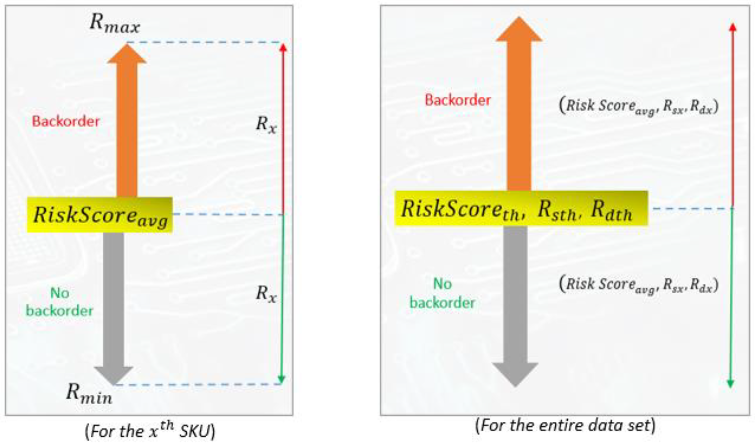
3.1.3. Notations

• The notations required for the formulation of the backorder problem in mathematical terms enable one to solve the model to find optimal solutions for the occurrence of backorder risk. The set represents the SKUs with common properties or characteristics essential for the mathematical expressions. The parameters are the fixed values in the mathematical model that represent the risk score. The variable represents the values of supplier performance and actual demand to be determined.

Sets

• $n$: Number of SKUs in the supply chain dataset.
• $x:$ The row number of the SKU under consideration. (It is used as an index or label to identify a specific row or entry within the dataset. In the context of the equations, x takes values from 1 to n, representing each SKU in the dataset. For each SKU, the equations are calculated based on the values associated with that specific SKU, such as supplier performance and actual demand. Such an index helps one iterate through each SKU in the dataset to calculate risk scores, constraints, and other relevant quantities).

Parameters

• $Riskscor{e}_{th}=$ Threshold of Risk score;
• $R_{sth}$ = Threshold of Total risk associated with Supplier Performance;
• $R_{dth}$ = Threshold of Total risk associated with Demand;
• $E_{spx}$ = Expected supplier performance for xth SKU;
• $A_{dx}$ = Actual demand for $\mathrm{xth}$ SKU.

Variables

• $V_{spx}$ = Variance in supplier performance for xth SKU;
• $V_{drx}$ = Variance in demand risk of xth SKU;
• $R_{sx}$ = Risk associated with Supplier Performance for the xth SKU;
• $R_{dx}$ = Risk associated with Actual Demand for the xth SKU;
• $Total Risk$ = Total risk related to the SKU associated with the supply chain;
• $Risk Scor{e}_{avg}$ = Average of total risk;
• $R{T}_s$ = Total Risk associated with Supplier Performance;
• $R{T}_d$ = Total Risk associated with Demand;
• $R_x$ = Risk score associated with both supplier performance and demand for the xth SKU;
• $R_{min}$ = Min value of $R_x$;
• $R_{max}$ = Max value of $R_x$.

From the root cause analysis conducted in Section 4, risks associated with Demand and Supplier Performance were found to be the root cause of back-order risks.

The below equations calculate the Variance in supplier performance and demand:

• $V_{spx}$ = Actual Supplier Performance–Expected Supplier Performance;
• $V_{drx}$ = Actual Demand–Expected Demand.

Equations (1) and (2) calculate the risk score for supplier performance and demand for the 1st to xth SKU in the dataset. They are calculated using the Mean Absolute Percentage Error (MAPE) method, where the modulus of variance for Supplier Performance and Demand is divided by Expected Performance and Demand.

$$R_{sx}=\left\{\frac{\mid Vspx\mid }{Espx}\right\}$$

(1)

$$R_{dx}=\left\{\frac{\mid Vdrx\mid }{Adx}\right\}$$

(2)

Equations (3) and (4) sum Equations (1) and (2) from the 1st SKU to the n^th SKU, calculating the total risk associated with supplier performance and demand in the supply chain from the 1st to the n^th SKU in the dataset.

$$R{T}_d={{\displaystyle \sum }}_{x=1}^n\cdot R_{dx}={{\displaystyle \sum }}_{x=1}^n\cdot \left\{\frac{\mid Vdrx\mid }{Adx}\right\}$$

(3)

Equations (5) and (6) calculate the Total Risk and $Risk Scor{e}_{avg}$ of all the SKUs in the supply chain dataset. Equation (5) was constructed by combining Equations (3) and (4) estimating the total risk associated with demand and supplier performance for the first to $n^{th}$ SKU. Equation (6) was obtained by dividing Equation (5) by $n$ (the total number of SKUs in the supply chain dataset); this yielded the average Risk Score, “$Risk Scor{e}_{avg}$”.

$$R{T}_s= {{\displaystyle \sum }}_{x=1}^n\cdot R_{sx}={{\displaystyle \sum }}_{x=1}^n\cdot \left\{\frac{\mid Vspx\mid }{Espx}\right\}$$

(4)

$$Total Risk={\displaystyle \sum }_{x=1}^n\cdot \left\{\left\{\frac{\mid Vspx\mid }{Espx}\right\}+\left\{\frac{\mid Vdrx\mid }{Adx}\right\}\right\}$$

(5)

$$Risk Scor{e}_{avg}=\frac{{{\displaystyle \sum }}_{x=1}^n\cdot \left\{\left\{\frac{\mid Vspx\mid }{Espx}\right\}+\left\{\frac{\mid Vdrx\mid }{Adx}\right\}\right\}}{n}$$

(6)

$R_x$ is calculated in Equation (7) by summing Equations (1) and (2). Equation (7) is the objective function. $R_x$ gives the risk score associated with the $x^{th}$ SKU item. $R_{min}$ and $R_{max}$ are calculated in Equations (8) and (9), yielding the Min Risk Score and Max Risk Score for $n$ SKUs. $R_{min}$ is calculated by minimizing the objective function of Equation (7), and $R_{max}$ is calculated by maximizing Equation (7).

$$R_x=R_{sx}+R_{dx}$$

(7)

$$R_{min}= mi{n}_{x=1}^n{R}_x$$

(8)

$$R_{max}= ma{x}_{x=1}^n{R}_x$$

(9)

Constraints

The constraints are shown in Equations (10)–(14).

$$R_{min}⩽R_x⩽RiskScor{e}_{avg}$$

(10)

$$RiskScor{e}_{avg}<R_x⩽R_{max}$$

(11)

$$R_{sx}⩽R_{sth}$$

(12)

$$R_{dx}⩽R_{dth}$$

(13)

$$Risk Scor{e}_{avg}⩽Riskscor{e}_{th}$$

(14)

If constraint (10) is met, then there is no possibility of supply chain risk for the $x^{th}$ SKU; in the case in which constraint (11) is satisfied, there is a possibility of supply chain risk for the $x^{th}$ SKU. If constraints (12)–(14) are not met, then there is a possibility of risk in the entire supply chain rather than for each SKU. The model’s constraints are shown in Figure 3.

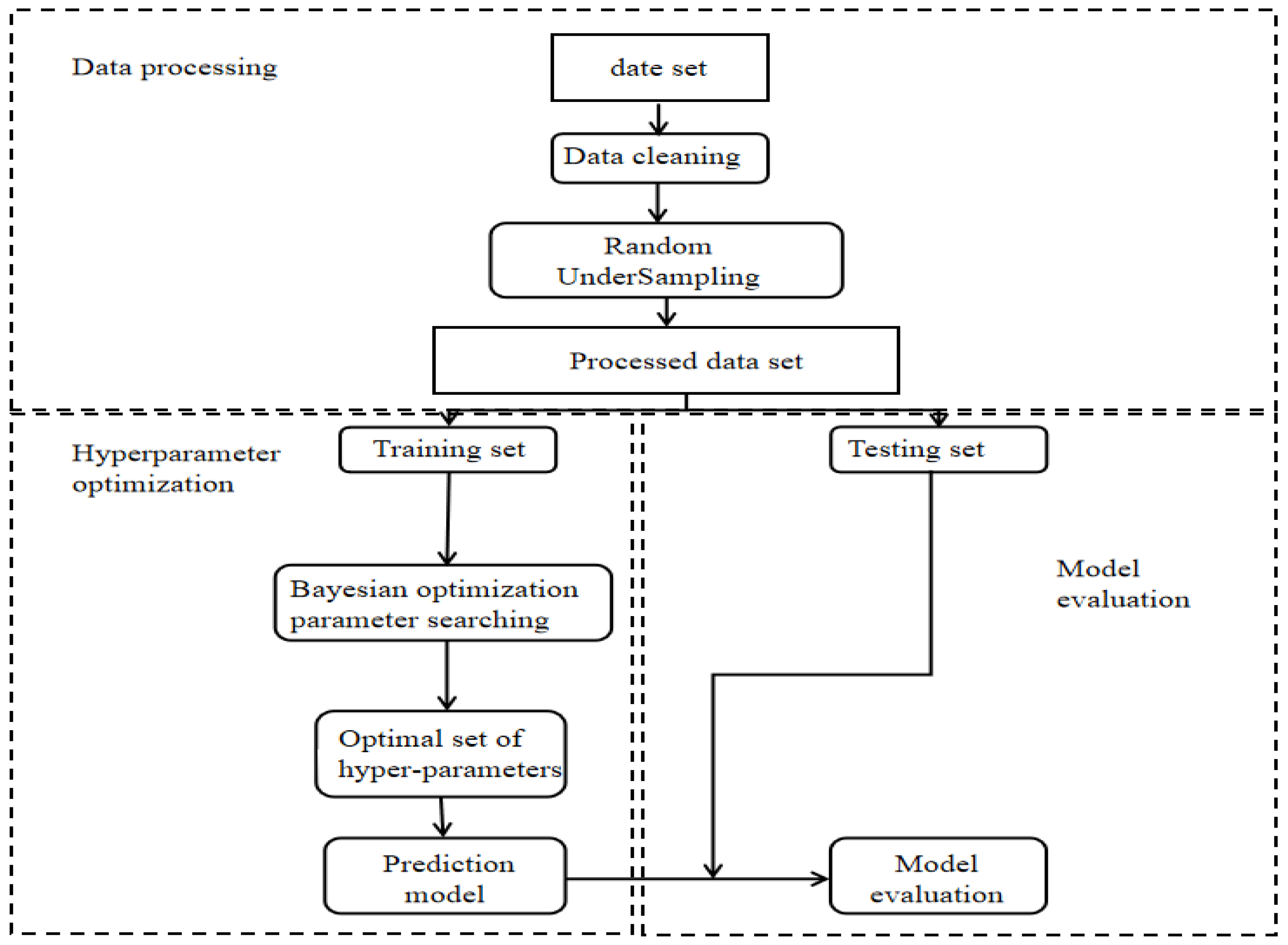
3.2. Machine Learning-Based Prediction Model

To predict the risk of supply chain delivery delays, the Bayesian-optimized LightGBM algorithm was employed in this research, as depicted in Figure 4. The choice of this algorithm is justified by several of the advantages it offers over other alternatives. Firstly, the Bayesian-optimized LightGBM algorithm exhibits high efficiency, enabling fast training and scalability for handling large-scale datasets. Secondly, it demonstrates superior predictive accuracy and performance compared to other algorithms, as supported by relevant studies [40]. Thirdly, this algorithm’s capabilities align well with supply chain delivery delay risk prediction requirements, including with respect to its ability to handle high-dimensional data, effectively manage missing data, and address class imbalance issues.

The specific steps of the proposed algorithm are illustrated below. Firstly, data pre-processing is conducted to ensure the integrity and availability of the dataset. Subsequently, the dataset is divided into training and testing sets proportionally. To address data imbalance, random under sampling is employed, randomly eliminating a majority of class samples from the training dataset until the number matches that of the minority class samples [41]. Finally, the classification model is trained using the training set. A Bayesian optimisation hyper-parameter search is employed to identify the optimal hyper-parameter. The model is then constructed using the testing set, and the model’s classification performance is evaluated. Data analysis and model development are carried out using Anaconda-based Python programming (version 3.8).

3.2.1. Data Pre-Processing

• Under-Sampling

The issue of classification imbalance can result in significant deviations in a model’s training outcomes. One effective algorithm for addressing class imbalance problems is the under-sampling method. This approach achieves a proportional balance between the remaining majority and minority class samples by removing a portion of the majority class samples [42]. Notably, this technique can enhance both the model’s generalization ability and operational efficiency, particularly when dealing with large datasets [43]. Additionally, under sampling guarantees that every data point originates directly from the initial dataset, which aids in preserving the authenticity of the data and reduces the potential for additional noise. One under-sampling algorithm, known as random under sampling, achieves class sample proportionality via randomly eliminating most class samples, and the balance ratio can be adjusted accordingly.

2.

Data Cleaning

As a crucial step in data analysis and mining, data pre-processing plays a vital role in enhancing the accuracy and effectiveness of data-mining results [44]. The specific process of data cleaning in this research includes the following steps: the integration of the training and testing sets, the removal of abnormal data, the deletion of missing values without compromising data quality, the elimination of redundant feature columns, and the conversion of data types, whereby string values such as ‘Yes’ and ‘No’ are replaced with 0/1 to facilitate analysis.

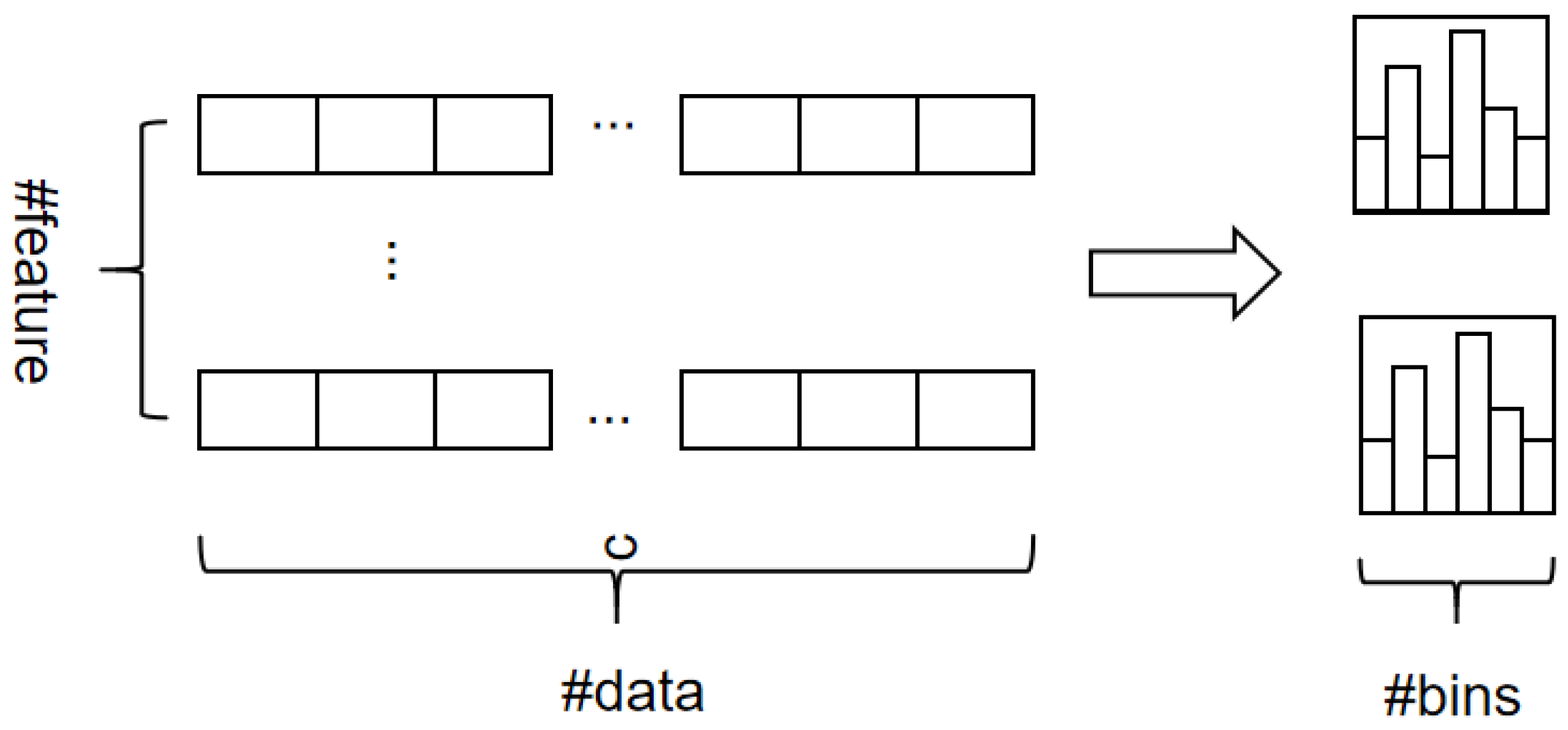
3.2.2. LightGBM Algorithm

The LightGBM algorithm is an open-source Gradient-Boosting Decision Tree (GBDT) framework [45]. The traditional GBDT model suffers from low efficiency and poor scalability when dealing with high-dimensional big data. The GBDT algorithm has been optimised to address these issues, and an improved version known as LightGBM has been introduced [46]. LightGBM introduces two key algorithms for improving training speed: the Histogram algorithm and the Gradient One-Side Sampling (GOSS) algorithm.

3.

The Histogram Algorithm

To address memory consumption and feature dimensionality, the LightGBM algorithm replaces the traditional pre-sorting algorithm with a histogram algorithm [47]. Figure 5 illustrates the process of discretising continuous eigenvalues into k eigenvalues and constructing a histogram with a width of k. When traversing the data, the cumulative value of each discrete value in the histogram is calculated, ultimately identifying the optimal segmentation point based on the traversal of the discrete value [48]. An overview of the histogram algorithm is provided in Algorithm 1 [48].

Algorithm 1 Histogram-based Algorithm

Input: training data I, max depth d, feature dimension m 1: nodeSet ← {0} ▷ tree nodes in current level 2: rowSet ← {{0, 1, 2}} ▷ data indices in tree nodes 3: for i = 1 to d do 4:  for node in nodeSet do 5:   usedRows ← rowSet[node] 6:   for k = 1 to m do 7:    H ← new Histogram() 8:    ▷ Build histogram 9:    for j in usedRows do 10:     bin ← I.f[k][j].bin 11:     H[bin].y ← H[bin].y + I.y[j] 12:     H[bin].y ← H[bin].y + 1 13:    end for 14:    Find the best split on histogram H 15:   end for 16:  end for 17:  Update rowSet and nodeSet according to the best split points 18: end for

4.

The GOSS Algorithm

In traditional GBDT algorithms, all sample points are used to calculate the gradient during sample sampling. However, computing the information gain for all sample points becomes time consuming when dealing with large datasets and high-dimensional features. LightGBM employs the GOSS algorithm for sampling to alleviate this issue and improve computational efficiency. The core idea behind GOSS is to retain large gradients while randomly sampling the remaining samples with slight gradients. A weight coefficient is introduced to calculate the information gain for the small gradient data to compensate for the impact on the sample points’ distribution. An overview of the GOSS algorithm is provided in Algorithm 2 [48].

Algorithm 2 Gradient-based One-side Sampling

Input: training data I, iterations d

Input: sampling ratio of large gradient data a

Input: sampling ratio of small gradient data b

Input: loss function loss, weak learner L

1: models ← { }, fact ← $\frac{1-a}{b}$

2: topN ← a $\times$ len(I), randN ← b $\times$ len(I)

3: for i = 1 to d do

4:  preds ← models.predict(I)

5:  g ← loss(I, preds), w ← {1, 1,…}

6:  sorted ← GetSortedIndices(abs(g))

7:  topSet ← sorted[1: topN]

8:  randSet ← RandomPick(sorted[topN : len(I)]), randN)

9:  usedSet ← topSet + randSet

10:   w[randSet] $\times =$ fact ▷ Assign weight fact to small gradient data

11:   newModel ← L(I[usedSet]), −g[usedSet], w[usedSet])

12:   model.append(newModel)

13: end for

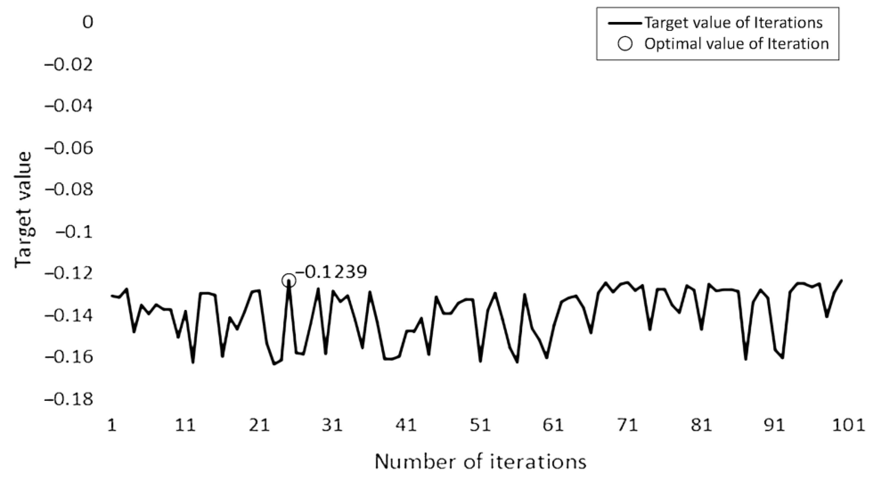
3.2.3. Bayesian Optimisation

The selection of hyperparameters is of utmost importance, as a well-chosen set of hyperparameters can significantly enhance a model’s performance [49]. Commonly employed methods for parameter tuning include manual adjustment, grid searches, random searches, and Bayesian optimisation [50]. The manual parameter adjustment method is time consuming and has difficulty identifying the best parameter combination through repeated trials. Grid searches and random searches, on the other hand, do not leverage prior information when evaluating hyperparameter combinations. Bayesian optimisation, however, utilises prior information from previous parameter sets to determine the next set to be evaluated, resulting in higher search efficiency with fewer iterations and the ability to swiftly and accurately find the optimal hyperparameter solution. This research employs the Bayesian optimisation algorithm to determine the optimal set of hyperparameters for the LightGBM model in predicting supply chain delivery delay risk [51].

3.2.4. Model Evaluation

The binary classifier employs the following evaluation criteria to assess its classification performance: overall classification accuracy and error rate [52]. To provide a comprehensive evaluation of the model’s performance, Precision and Recall were also chosen as evaluation metrics [48]. The model’s Accuracy, Precision, and Recall rates are calculated based on a confusion matrix [53]. In

Table 1. Confusion matrix.

True Result	Prediction Result
	Negative	Positive
Negative	True Negative (TN)	False Positive (FP)
Positive	False Negative (FN)	True Positive (TP)

, TN represents the number of samples where both the real result and the predicted result are negative. TP represents the number of samples where both the real result and the predicted result are positive. FN corresponds to the number of samples where the real result is positive, but the predicted result is negative. FP denotes the number of samples where the real result is negative, but the predicted result is positive.

The accuracy rate denotes the probability of correctly predicting both positive and negative classes across all samples, as shown in Equation (15).

$$Accuracy=\frac{TN+TP}{TN+TP+FN+FP}$$

(15)

The Precision rate denotes the proportion of correctly identified positive samples out of all the predicted positive samples, as shown in Equation (16).

$$Precision=\frac{TP}{TP+FP}$$

(16)

The Recall rate refers to the likelihood of a sample being correctly identified as a positive sample among the actual positive samples, as shown in Equation (17).

$$Recall=\frac{TP}{TP+TN}$$

(17)

Furthermore, the model’s performance is assessed using the area under the receiver operating characteristic curve (ROC), commonly referred to as area under curve (AUC) [54]. The AUC serves as an indicator that reflects a binary classifier’s ability to accurately classify positive and negative samples. This metric allows for an assessment of a model’s performance across different class boundary values and tests its robustness in cases of imbalanced datasets. Additionally, each machine learning model’s operation time is considered an evaluation metric in this research.

4. Empirical Study

In the realm of the supply chain, backorders represent a significant risk to timely delivery. A backorder can arise from various factors, including supplier management, material transportation capabilities, supplier evaluation processes, and unforeseen circumstances. Backorders within a supply chain can result in substantial losses due to a failure to deliver products punctually. Therefore, the backorder data serve to validate the efficacy of the proposed Bayesian-optimized LightGBM algorithm.

4.1. Data Description

In this research, an actual 8-week imbalanced historical dataset pertaining to product backorders was used [55]. The data were collected through a weekly survey conducted at the beginning of each week, resulting in a highly skewed distribution with an imbalance ratio of 1:137. The dataset comprises 13,981 positive samples and 1,915,954 negative samples. Comprehensive definitions of the attributes present in the dataset are provided in

Table 2. The definitions of the attributes.

Attributes	Ranges	Explanation
went_on_back_order (Binary)	Binary (0 or 1)	Product went on backorder
forecast_3_month, forecast_6_month, forecast_9_month (parts)	0–138,240	Sales forecast for next 3, 6, and 9 months
sales_1_month, sales_3_month, sales_6_month, sales_9_month (parts)	0–132,068	Sales volume in last 1, 3, 6, and 9 months
perf_6_month_avg, perf_12_month_avg (%)	0 to 100%	Supplier performance in last 6 and 12 months
min_bank (parts)	0–9672	Minimum recommended stock amount
pieces_past_due (parts)	0	Number of parts overdue from supplier
local_bo_qty (parts)	0	Amount of stock overdue
in_transit_qtry (parts)	0–5562	Quantity in transit
lead_time (days)	2 to 52	Transit time
national_inv (parts)	0–266,511	Current inventory level
potential_issue (Binary)	Binary (0 or 1)	Identified source issue for the item
deck_risk, stop_auto_buy, rev_stop (Binary)	Binary (0 or 1)	General risk indicators
oe_constraint (Binary)	Binary (0 or 1)	Constraints on operating entities
ppap_risk (Binary)	Binary (0 or 1)	Risk associated with the production part approval process

. Furthermore, a visual representation of the dataset within the supply chain framework is shown in Figure 6.

The results of the correlation analysis conducted on these attributes are shown in Figure 7. The thermal value is 1, signifying a strong correlation between the two data variables. Conversely, a correlation is absent between the two data variables in cases where the thermal value is 0. Despite the weak correlation observed between the target attribute “went_on_backorder” and the other variables, it was essential to consider all variables in this research. By integrating all the features, a model can be more robust and generalizable across various datasets and scenarios.

Furthermore, a data feature analysis was conducted to identify the top ten features that have a significant impact on the outcomes, as shown in Figure 8. The most influential factor affecting delayed delivery is the current inventory of the product. This factor is followed closely by the performance of suppliers and sales performance in recent months, aligning with real-world observations.

4.2. Data Pre-Processing

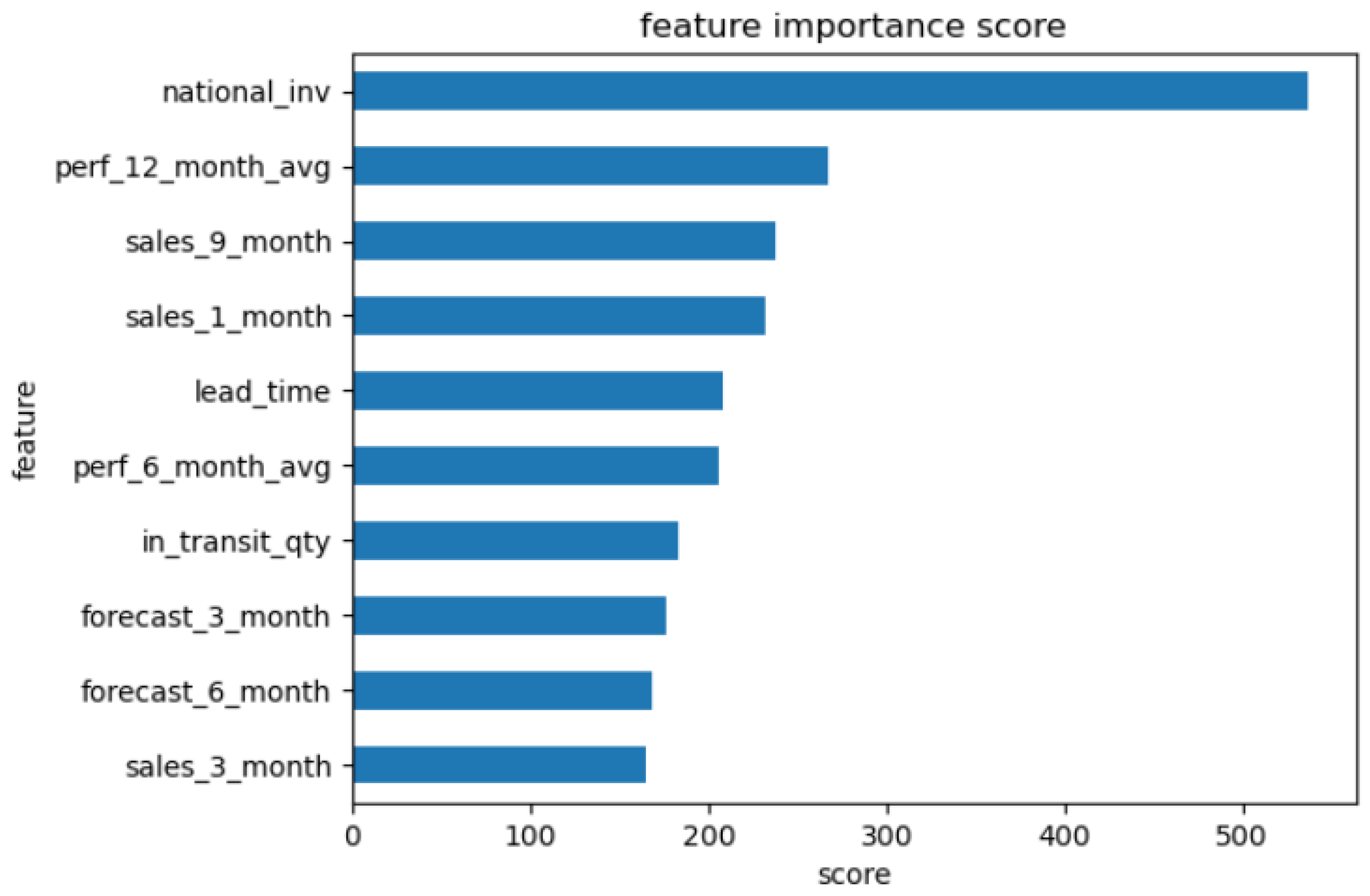
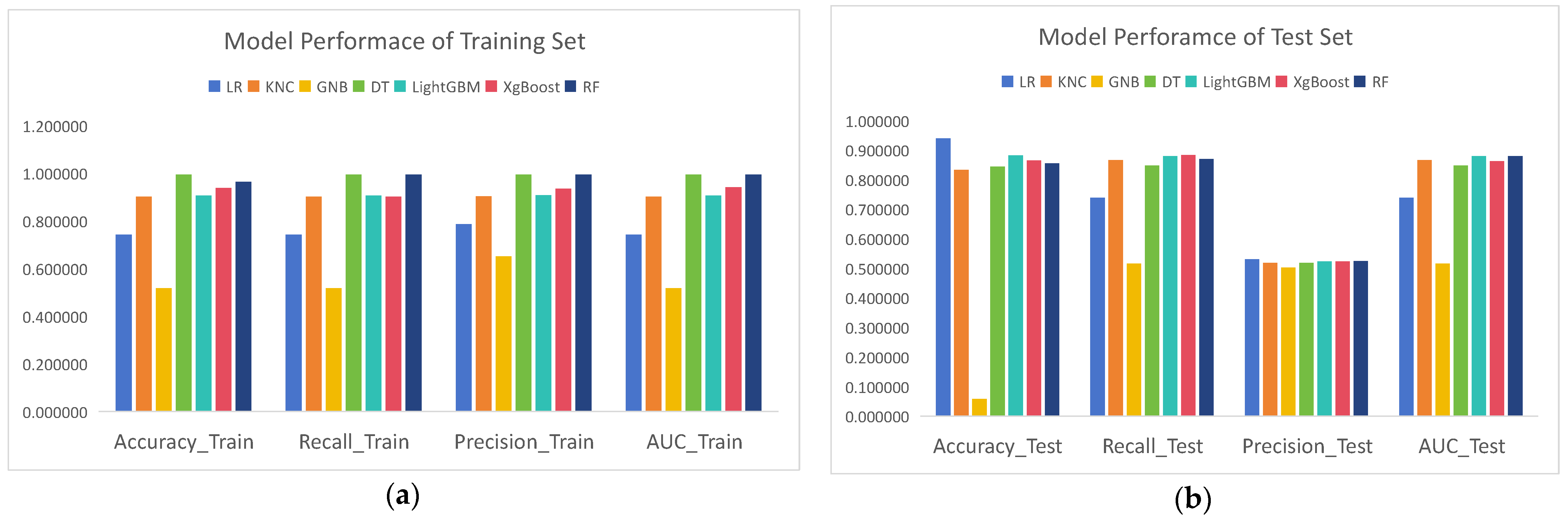
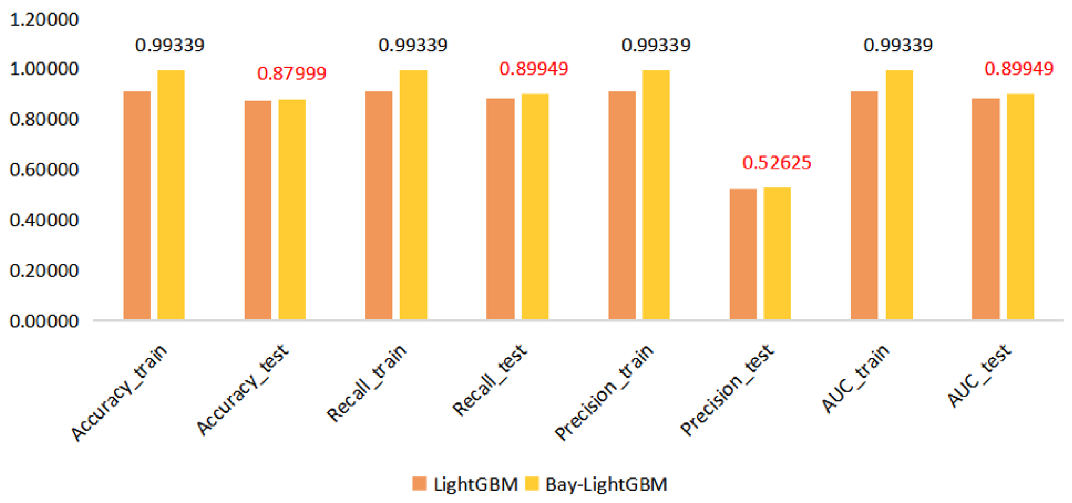
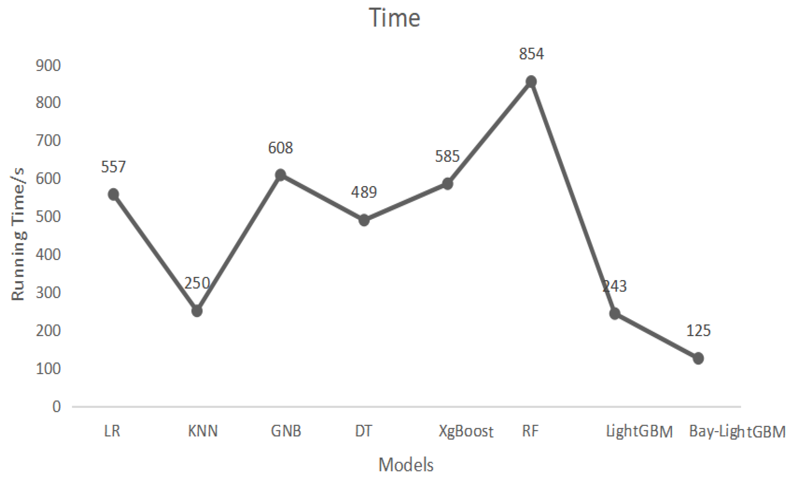
The dataset was partitioned into training and testing sets in a ratio of 7:3 [32]. Given the significant class imbalance of the initial dataset, random under sampling was performed on the training set to mitigate the influence of this imbalance. The original dataset and the dataset after random under sampling are both shown in

Table 3. Positive and negative sample results from the dataset.

Type	Original Dataset			Dataset after Random under Sampling
	True Sample	False Sample	Overall	True Sample	False Sample	Overall
Training set	1,341,197	9757	1,350,954	9757	9757	19,514
Test set	574,801	4180	578,981	574,801	4180	578,981
Overall	1,915,998	13,937	1,929,935	584,558	13,937	598,495

. In this table, samples without backorders are considered positive, while those with backorders are considered harmful.

4.3. Model Building

To address the effectiveness, robustness, and accuracy of the model in handling large samples and high-dimensional datasets, seven machine learning models are compared in this research, namely, logical regression (LR), k-nearest neighbour (KNN), naive Bayes (GaussianNB, GNB), decision tree (DT), random forest (RF), XGBoost, and LightGBM. These models were chosen based on their common usage in related literature and widespread adoption in practical applications. The performance of these models for the training and testing sets is depicted in Figure 9.

It is evident that the GNB model exhibits the poorest classification performance when dealing with highly imbalanced data, as indicated by its accuracy of only 0.5 for the training set. This can be attributed to the Naive Bayesian model’s advantage in modelling small samples. However, this advantage diminishes when confronted with datasets containing a substantial quantity of data, resulting in poor generalization ability. These findings are consistent with those from previous studies [56,57]. Though both the RF model and XGBoost model achieve a high level of accuracy when compared to the LightGBM model, it is worth noting that the LightGBM model demonstrates superior computational efficiency and lower memory usage for large datasets [46]. Therefore, the LightGBM model exhibits outstanding performance. To further enhance the performance of the LightGBM model, the optimal set of hyperparameters was determined through continuous iterative optimisation using Bayesian optimisation. The objective function utilized for optimisation was the mean squared error value of five-fold cross-validation, which was within a given range of hyperparameters. Considering the desire to achieve a good balance between optimisation efficiency and accuracy, the optimisation process consists of 100 controlled iterations and 50 random iterations. The mean squared error curve of the training set with respect to the target is illustrated in Figure 10. The Bayesian hyperparameter optimisation reaches the optimal value at the 25th iteration, which is −0.1239. It is important to note that even though the iteration count may appear relatively low, further iterations did not lead to significant improvements in the optimisation results. In fact, Bayesian optimization is designed to make informed decisions based on prior data. Its goal is to find the optimal solution with fewer iterations, making the selected iteration count appropriate for our specific problem. Consequently, the optimal set of LightGBM hyperparameters is presented in

Table 4. The optimal set of LightGBM hyperparameters.

Parameter	max_Depth	n_ Estimators	reg_alpha	min_child_ Samples	num_ Leaves	reg_ Lambda	Subsample
Value	10	2930	0.1	47	20	1.0	0.8

.

The performance of LightGBM was compared with and without Bayesian optimisation (see Figure 11). Furthermore, the respective operation times of each model were also compared (see Figure 12). Additionally, the AUC score was utilised to assess the performance of the Bayesian-optimized LightGBM model compared to other models. The AUC score represents the probability of a given classifier ranking a random positive example higher than a random negative example, and it is computed by calculating the area under the ROC curve, as presented in Figure 13.

Compared to the LightGBM model, the Bayesian-optimized LightGBM (BO-LightGBM) model exhibited higher accuracy, recall, and AUC values, which were 0.88, 0.89, and 0.89, respectively, when predicting the risk of backorder. Considering the ACU score and operational time of all the models, it is evident that the RF model outperforms the others. However, it is important to note that RF requires a longer running time and occupies more memory compared to LightGBM and XGBoost. Despite being an efficient implementation of GBDT, the performance of XGBoost still falls short of the model proposed in this research. The results demonstrate that the proposed BO-LightGBM model not only significantly enhances the model’s classification performance, stability, and generalisation ability, with an AUC score of 0.957, but also exhibits the shortest operational time of 125 s. This model effectively predicts backorder risk, especially in scenarios involving large samples, high dimensions, and imbalanced datasets.

5. Discussion

Predicting supply chain delay risks is valuable for effective supply chain management and inventory planning. It empowers retailers to manage inventory levels and proactively prevent stockouts. In this study, we proposed a Bayesian-optimized LightGBM model based on the random under-sampling method for data pre-processing, aiming to predict the occurrence of supply chain delay risks.

To validate the proposed model, we utilised a backorder dataset as a representative example of delivery delay risks within a supply chain, for which 21 indicators were considered, including lead time, inventory, and sales. Analysing backorder data can provide valuable insights for improving inventory management and forecasting via identifying relevant trends. To investigate the factors contributing to the risk of backorders, we conducted correlation analysis to visualise the variables and found that all the variables are associated with risk. In addition, we performed a rigorous analysis to evaluate and rank the factors contributing to the emergence of supply chain risk. The findings demonstrate that the current inventory level significantly impacts the incidence of backorder risk. Moreover, it was discovered that the past performance of suppliers over the last twelve months and previous sales records considerably influence the probability of a backorder.

First, seven machine learning models were compared in this study: logical regression (LR), k-nearest neighbour (KNN), naive Bayes (GaussianNB, GNB), decision tree (DT), random forest (RF), XGBoost, and LightGBM. These models were chosen based on their common usage in the related literature and widespread adoption in practical applications. It is evident that the GNB model exhibits the poorest classification performance when dealing with highly imbalanced data, as indicated by its accuracy of only 0.5. However, although both the RF and XGBoost models achieve a high level of accuracy when compared to the LightGBM model, it is worth noting that the LightGBM model demonstrates superior computational efficiency and lower memory usage for large datasets. Therefore, the LightGBM model exhibits outstanding performance. The performance of the LightGBM model was further enhanced through continuous iterative optimisation using Bayesian optimisation.

Next, we compared the accuracy and operational time of the proposed Bayesian-optimized LightGBM model. The results demonstrate that the BO-LightGBM model exhibits higher accuracy and operates in the shortest time, indicating its superior prediction performance for supply chain delivery delay risk and strong generalisation ability. Moreover, the results show that the BO-LightGBM model can handle large sample sizes and imbalanced datasets effectively. The implications of our analysis are of utmost importance as they offer valuable insights to supply chain managers, empowering them to devise effective strategies for mitigating the risk of product delivery delay in the supply chain and enhancing the overall resilience of the supply chain ecosystem. However, this research does have some limitations. Factors such as weather conditions, geographical factors, and regional influences, which are prevalent in the supply chain, have not been considered. Future work should focus on incorporating these factors into analyses. Gathering real-time stock-level data is crucial to implement the proposed prediction model in practical settings. This necessitates integrating advanced technology into warehouse inventory systems. Once the prediction system is implemented, it can send real-time notifications and alerts to inventory and production management regarding potential backorder issues, enabling timely restocking from suppliers. Future work should also focus on further investigating such an automated early-warning system to mitigate the occurrence of supply chain delivery delay risks.

6. Conclusions

Applying a Machine Learning-based Bayesian-optimized LightGBM model has demonstrated significant promise in predicting and mitigating supply chain risks in the context of Industry 4.0. Supply chain risk management has become a crucial aspect of modern business operations, as disruptions can lead to substantial financial losses and reputational damage. Leveraging machine learning techniques and Bayesian optimisation within the LightGBM framework, this research has paved the way for a proactive and data-driven approach to identifying, assessing, and responding to potential risks in supply chains. The predictive power of the proposed model is attributed to its ability to analyse vast quantities of historical data and extract complex patterns and relationships. By leveraging historical data, the model can make accurate risk forecasts, enabling organisations to take timely and informed actions to mitigate potential disruptions.

The findings of this research align with the growing body of literature that emphasises the value of machine learning approaches in supply chain risk management. Other studies have shown that machine learning-based models, such as deep learning and Random Forest, can also provide accurate and efficient risk predictions. However, the proposed Bayesian-optimized LightGBM model introduces a unique combination of techniques that offers improved performance and interpretability, making it a compelling choice for organisations seeking to enhance their risk management practices. While this study has provided valuable insights into the effectiveness of Supply Chain 4.0 in predicting supply chain risk, further research is encouraged to explore its applicability in diverse industries and supply chain settings. Additionally, investigations into the model’s scalability and adaptability to real-time data streams would contribute to its practical implementation in dynamic and rapidly changing supply chain environments.

Overall, the integration of machine learning techniques into supply chain risk management marks a significant advancement in the field. The developed model, with its Bayesian-optimized LightGBM approach, demonstrates the potential to revolutionize how organisations proactively manage and navigate supply chain disruptions. As businesses continue to embrace digital transformation and Industry 4.0 principles, the adoption of advanced predictive analytics and data-driven strategies will be instrumental in building resilient and efficient supply chains, securing competitive advantages, and sustaining success in an increasingly complex and interconnected global marketplace.

References

1. MacKenzie, C.A.; Barker, K.; Santos, J.R. Modeling a severe supply chain disruption and post-disaster decision making with application to the Japanese earthquake and tsunami. IIE Trans. 2014, 46, 1243–1260. [Google Scholar] [CrossRef]
2. Ivanov, D. Predicting the impacts of epidemic outbreaks on global supply chains: A simulation-based analysis on the coronavirus outbreak (COVID-19/SARS-CoV-2) case. Transp. Res. Part E Logist. Transp. Rev. 2020, 136, 101922. [Google Scholar] [CrossRef] [PubMed]
3. Arto, I.; Andreoni, V.; Rueda Cantuche, J.M. Global impacts of the automotive supply chain disruption following the Japanese earthquake of 2011. Econ. Syst. Res. 2015, 27, 306–323. [Google Scholar] [CrossRef]
4. Burstein, G.; Zuckerman, I. Deconstructing Risk Factors for Predicting Risk Assessment in Supply Chains Using Machine Learning. J. Risk Financ. Manag. 2023, 16, 97. [Google Scholar] [CrossRef]
5. Tang, J.; Haddad, Y.; Salonitis, K. Reconfigurable manufacturing system scheduling: A deep reinforcement learning approach. Procedia CIRP 2022, 107, 1198–1203. [Google Scholar] [CrossRef]
6. Tang, J.; Salonitis, K. A deep reinforcement learning based scheduling policy for reconfigurable manufacturing systems. Procedia CIRP 2021, 103, 1–7. [Google Scholar] [CrossRef]
7. Alrufaihi, D.; Oleghe, O.; Almanei, M.; Jagtap, S.; Salonitis, K. Feature reduction and selection for use in machine learning for manufacturing. Adv. Transdiscipl. Eng. 2022, 25, 289–296. [Google Scholar] [CrossRef]
8. Almanei, M.; Oleghe, O.; Jagtap, S.; Salonitis, K. Machine learning algorithms comparison for manufacturing applications. Adv. Manuf. Technol. 2021, 34, 377–382. [Google Scholar] [CrossRef]
9. Guo, L.; Wang, Y.; Kong, D.; Zhang, Z.; Yang, Y. Decisions on spare parts allocation for repairable isolated system with dependent backorders. Comput. Ind. Eng. 2019, 127, 8–20. [Google Scholar] [CrossRef]
10. Beam, A.L.; Kohane, I.S. Big data and machine learning in health care. JAMA 2018, 319, 1317–1318. [Google Scholar] [CrossRef]
11. Ni, D.; Xiao, Z.; Lim, M.K. A systematic review of the research trends of machine learning in supply chain management. Int. J. Mach. Learn. Cybern. 2020, 11, 1463–1482. [Google Scholar] [CrossRef]
12. Bavarsad, B.; Boshagh, M.; Kayedian, A. A study on supply chain risk factors and their impact on organizational Performance. Int. J. Oper. Logist. Manag. 2014, 3, 192–211. [Google Scholar]
13. Schroeder, M.; Lodemann, S. A systematic investigation of the integration of machine learning into supply chain risk management. Logistics 2021, 5, 62. [Google Scholar] [CrossRef]
14. Shekarian, M.; Mellat Parast, M. An Integrative approach to supply chain disruption risk and resilience management: A literature review. Int. J. Logist. Res. Appl. 2021, 24, 427–455. [Google Scholar] [CrossRef]
15. Gaudenzi, B.; Borghesi, A. Managing risks in the supply chain using the AHP method. Int. J. Logist. Manag. 2006, 17, 114–136. [Google Scholar] [CrossRef]
16. Salamai, A.; Hussain, O.K.; Saberi, M.; Chang, E.; Hussain, F.K. Highlighting the importance of considering the impacts of both external and internal risk factors on operational parameters to improve Supply Chain Risk Management. IEEE Access 2019, 7, 49297–49315. [Google Scholar] [CrossRef]
17. Ho, W.; Zheng, T.; Yildiz, H.; Talluri, S. Supply chain risk management: A literature review. Int. J. Prod. Res. 2015, 53, 5031–5069. [Google Scholar] [CrossRef]
18. MacKenzie, C.A.; Santos, J.R.; Barker, K. Measuring changes in international production from a disruption: Case study of the Japanese earthquake and tsunami. Int. J. Product. Econ. 2012, 138, 293–302. [Google Scholar] [CrossRef]
19. DuHadway, S.; Carnovale, S.; Hazen, B. Understanding risk management for intentional supply chain disruptions: Risk detection, risk mitigation, and risk recovery. Appl. OR Disaster Relief Oper. 2019, 283, 179–198. [Google Scholar] [CrossRef]
20. Nikookar, E.; Varsei, M.; Wieland, A. Gaining from disorder: Making the case for antifragility in purchasing and supply chain management. J. Purch. Supply Manag. 2021, 27, 100699. [Google Scholar] [CrossRef]
21. Ponis, S.T.; Koronis, E. Supply Chain Resilience? Definition of concept and its formative elements. J. Appl. Bus. Res. 2012, 28, 921–935. [Google Scholar] [CrossRef]
22. Ponomarov, S. Antecedents and Consequences of Supply Chain Resilience: A Dynamic Capabilities Perspective. Ph.D. Thesis, University of Tennessee, Knoxville, TN, USA, 2012. [Google Scholar]
23. Kleijnen, J.P.; Smits, M.T. Performance metrics in supply chain management. J. Oper. Res. Soc. 2003, 54, 507–514. [Google Scholar] [CrossRef]
24. Björk, K.-M. An analytical solution to a fuzzy economic order quantity problem. Int. J. Approx. Reason. 2009, 50, 485–493. [Google Scholar] [CrossRef]
25. Kazemi, N.; Ehsani, E.; Jaber, M.Y. An inventory model with backorders with fuzzy parameters and decision variables. Int. J. Approx. Reason. 2010, 51, 964–972. [Google Scholar] [CrossRef]
26. Feng, G.; Chen-Yu, L.; Feng-Lei, X.; Wei-Ling, L. Demand Prediction of LRU Parts with Backorder for SRU. In Proceedings of the 2012 Fifth International Symposium on Computational Intelligence and Design, Hangzhou, China, 28–29 October 2012; pp. 530–532. [Google Scholar] [CrossRef]
27. Lee, H.L. The Triple-A Supply Chain. Harv. Bus. Rev. 2004, 82, 102–113. [Google Scholar]
28. Disney, S.M.; Towill, D.R. On the bullwhip and inventory variance produced by an ordering policy. Omega 2003, 31, 157–167. [Google Scholar] [CrossRef]
29. Nahmias, S.; Olsen, T.L. Production and Operations Analysis; Waveland Press: Long Grove, IL, USA, 2015. [Google Scholar]
30. Monczka, R.M.; Handfield, R.B.; Giunipero, L.C.; Patterson, J.L. Purchasing and Supply Chain Management; Cengage Learning: Boston, MA, USA, 2020. [Google Scholar]
31. Islam, S.; Amin, S.H. Prediction of probable backorder scenarios in the supply chain using Distributed Random Forest and Gradient Boosting Machine learning techniques. J. Big Data 2020, 7, 65. [Google Scholar] [CrossRef]
32. Ntakolia, C.; Kokkotis, C.; Karlsson, P.; Moustakidis, S. An explainable machine learning model for material backorder prediction in inventory management. Sensors 2021, 21, 7926. [Google Scholar] [CrossRef]
33. De Santis, R.B.; de Aguiar, E.P.; Goliatt, L. Predicting material backorders in inventory management using machine learning. In Proceedings of the IEEE Latin American Conference on Computational Intelligence (LA-CCI), Arequipa, Peru, 8–10 November 2017; pp. 1–6. [Google Scholar] [CrossRef]
34. Shajalal, M.; Hajek, P.; Abedin, M.Z. Product backorder prediction using deep neural network on imbalanced data. Int. J. Prod. Res. 2023, 61, 302–319. [Google Scholar] [CrossRef]
35. Hajek, P.; Abedin, M.Z. A profit function-maximizing inventory backorder prediction system using big data analytics. IEEE Access 2020, 8, 58982–58994. [Google Scholar] [CrossRef]
36. Sherwin, M.D.; Medal, H.; Lapp, S.A. Proactive cost-effective identification and mitigation of supply delay risks in a low volume high value supply chain using fault-tree analysis. Int. J. Prod. Econ. 2016, 175, 153–163. [Google Scholar] [CrossRef]
37. Ruijters, E.; Stoelinga, M. Fault tree analysis: A survey of the state-of-the-art in modeling, analysis and tools. Comput. Sci. Rev. 2015, 15, 29–62. [Google Scholar] [CrossRef]
38. Lee, W.-S.; Grosh, D.L.; Tillman, F.A.; Lie, C.H. Fault tree analysis, methods, and applications ߝ a review. ITR 1985, 34, 194–203. [Google Scholar] [CrossRef]
39. Xing, L.; Amari, S.V. Fault Tree Analysis. In Handbook of Performability Engineering; Springer: London, UK, 2008; pp. 595–620. [Google Scholar]
40. Hao, X.; Zhang, Z.; Xu, Q.; Huang, G.; Wang, K.J. Prediction of f-CaO content in cement clinker: A novel prediction method based on LightGBM and Bayesian optimization. Chemom. Intell. Lab. Syst. 2022, 220, 104461. [Google Scholar] [CrossRef]
41. Prusa, J.; Khoshgoftaar, T.M.; Dittman, D.J.; Napolitano, A. Using random undersampling to alleviate class imbalance on tweet sentiment data. In Proceedings of the 2015 IEEE International Conference on Information Reuse and Integration, San Francisco, CA, USA, 13–15 August 2015; pp. 197–202. [Google Scholar] [CrossRef]
42. Tanha, J.; Abdi, Y.; Samadi, N.; Razzaghi, N.; Asadpour, M. Boosting methods for multi-class imbalanced data classification: An experimental review. J. Big Data 2020, 7, 70. [Google Scholar] [CrossRef]
43. Ramyachitra, D.; Manikandan, P. Imbalanced dataset classification and solutions: A review. Int. J. Comput. Bus. Res. 2014, 5, 1–29. [Google Scholar]
44. Xu, S.; Lu, B.; Baldea, M.; Edgar, T.F.; Wojsznis, W.; Blevins, T.; Nixon, M. Data cleaning in the process industries. Rev. Chem. Eng. 2015, 31, 453–490. [Google Scholar] [CrossRef]
45. Chen, C.; Zhang, Q.; Ma, Q.; Yu, B. LightGBM-PPI: Predicting protein-protein interactions through LightGBM with multi-information fusion. Chemom. Intell. Lab. Syst. 2019, 191, 54–64. [Google Scholar] [CrossRef]
46. Al Daoud, E. Comparison between XGBoost, LightGBM and CatBoost using a home credit dataset. Int. J. Comput. Inf. Eng. 2019, 13, 6–10. [Google Scholar] [CrossRef]
47. Zeng, H.; Yang, C.; Zhang, H.; Wu, Z.; Zhang, J.; Dai, G.; Babiloni, F.; Kong, W. A lightGBM-based EEG analysis method for driver mental states classification. Comput. Intell. Neurosci. 2019, 2019, 3761203. [Google Scholar] [CrossRef]
48. Ke, G.; Meng, Q.; Finley, T.; Wang, T.; Chen, W.; Ma, W.; Ye, Q.; Liu, T.-Y. Lightgbm: A highly efficient gradient boosting decision tree. In Proceedings of the 2017 Conference on Neural Information Processing Systems, Long Beach, CA, USA, 4–9 December 2017; p. 30. [Google Scholar]
49. Frazier, P.I. Bayesian Optimization. In Recent Advances in Optimization and Modeling of Contemporary Problems; Informs: Scottsdale, AZ, USA, 2018; pp. 255–278. [Google Scholar]
50. Eriksson, D.; Pearce, M.; Gardner, J.; Turner, R.D.; Poloczek, M. Scalable global optimization via local bayesian optimization. In Proceedings of the Advances in Neural Information Processing Systems 32, Vancouver, BC, Canada, 8–14 December 2019; p. 32. [Google Scholar]
51. Wang, Z.; Zoghi, M.; Hutter, F.; Matheson, D.; De Freitas, N. Bayesian Optimization in High Dimensions via Random Embeddings. In Proceedings of the IJCAI, Beijing, China, 3–9 August 2013; pp. 1778–1784. [Google Scholar] [CrossRef]
52. Buckland, M.; Gey, F. The relationship between recall and precision. J. Am. Soc. Inf. Sci. 1994, 45, 12–19. [Google Scholar] [CrossRef]
53. Ehrig, M.; Euzenat, J. Relaxed precision and recall for ontology matching. In Proceedings of the K-CAP 2005 Workshop on Integrating Ontology, Banff, AL, Canada, 2 October 2005; pp. 25–32. [Google Scholar]
54. Tatbul, N.; Lee, T.J.; Zdonik, S.; Alam, M.; Gottschlich, J. Precision and recall for time series. In Proceedings of the 32nd Conference on Neural Information Processing Systems (NeurIPS 2018), Montreal, QC, Canada, 3–8 December 2018; p. 31. [Google Scholar]
55. Predictive Backorder Competition. Available online: https://github.com/rodrigosantis1/backorder_prediction (accessed on 1 March 2023).
56. Tzanos, G.; Kachris, C.; Soudris, D. Hardware acceleration on gaussian naive bayes machine learning algorithm. In Proceedings of the 2019 8th International Conference on Modern Circuits and Systems Technologies (MOCAST), Thessaloniki, Greece, 13–15 May; pp. 1–5. [CrossRef]
57. Huang, Y.; Li, L. Naive Bayes classification algorithm based on small sample set. In Proceedings of the 2011 IEEE International Conference on Cloud Computing and Intelligence Systems, Beijing, China, 15–17 September 2011; pp. 34–39. [Google Scholar] [CrossRef]
Figure 1. Methodology.
Machines 11 00888 g001
Figure 2. Fault tree diagram.
Machines 11 00888 g002
Figure 3. Risk score constraints.
Machines 11 00888 g003
Figure 4. Flow chart of the proposed supply chain risk prediction process.
Machines 11 00888 g004
Figure 5. The process of the histogram algorithm.
Machines 11 00888 g005
Figure 6. The dataset in the supply chain framework.
Machines 11 00888 g006
Figure 7. Correlation analysis.
Machines 11 00888 g007
Figure 8. Feature importance scores.
Machines 11 00888 g008
Figure 9. (a) Model performance for training set; (b) model performance for testing set.
Machines 11 00888 g009
Figure 10. Number of iterations required to find the optimal value.
Machines 11 00888 g010
Figure 11. The performance of LightGBM with and without Bayesian optimisation.
Machines 11 00888 g011
Figure 12. Operation times of different models.
Machines 11 00888 g012
Figure 13. AUC values for different models.
Machines 11 00888 g013