1. Introduction
Mechatronics integrates mechanical engineering (ME), electronic engineering (EE), information technology (IT), and control systems (CS) to reach an integrated approach involved in the design, manufacturing, and development of engineering systems [
1]. Adopting this methodology has resulted in noteworthy progress in numerous industries, such as precision engineering, aerospace, medical equipment design, and robotics applications [
2,
3].
In the field of mechatronics, CS play a crucial role in comprehending and designing complex systems, including diverse aspects such as feedback, robustness, dynamics, and decision-making. Deep comprehension of CS enables us to resolve some of the most pressing issues by developing innovative technologies and solutions [
4], adjusting the behavior of automated systems to operate within determined parameters and meet expected performance criteria [
5], and reaching enhanced accuracy, safety, and efficiency while reducing the likelihood of errors and system failures [
6].
Therefore, from an educational perspective, CS sciences are necessary to produce a new generation of engineers to design, develop, and control mechatronic systems. Equipping students with the necessary skills is of the utmost importance for mechatronics education as it prepares them to fulfill the demands of the modern industrial landscape [
4].
CS education requires interdisciplinary knowledge involving mathematical modeling, analytical thinking, computational skills, hardware development, and control design. According to [
1,
7,
8], it is essential to assess the balance between two main scenarios to succeed in mechatronics: the theoretical framework of mathematical modeling, analysis, and control design for dynamic physical systems and the empirical validation of these concepts.
The aforementioned process is analogous to the philosophy of STEM education (science, technology, engineering, and mathematics), where “know-what” (knowledge associated with the discipline) and the “know-how” (the skills to apply knowledge) result in the development of comprehensive learning [
9].
This philosophy can also be employed in the field of CS in this sense by assessing the required balance between theoretical and empirical validation, thus enabling students to apply their knowledge to address real-world challenges effectively. At the same time, STEM focuses on developing critical thinking, problem-solving, creativity, and collaboration skills, which are essential for success in any field, including mechatronics and other engineering disciplines [
10].
A practical method to achieve this is by providing a hands-on learning experience. According to the classical constructionism theory [
11], technology integration in hands-on learning actively involves students constructing their knowledge instead of being mere passive receptors of information.
This study aims to design, implement, and control an educational electrical linear actuator for teaching kinematics concepts. Linear actuators are valuable instruments for achieving precise linear motion. They have been extensively utilized in various applications, including automated vehicle drivers [
12], soft-robot actuators [
13], prosthetics and rehabilitation [
14], and automotive technology [
15]. Therefore, linear electric actuators provide an excellent prospect for students to learn about motion control, dynamics, and kinematics, crucial aspects of control systems frequently employed in automation. This proposal follows a modular approach suitable for educational purposes and includes an instructional design supported by software for constructing mechatronic concepts implicated in the determination of the motion of a particle, specifically the concept of uniform rectilinear motion; a fuzzy control is applied in the close loop. The proposal employs computer vision technology to retrieve the linear actuator;s position while developing pedagogical experiments.
The novelty of this work relies on a combination of educational tools incorporating computer vision (CV) and fuzzy control techniques, as well as the Educational Mechatronics Conceptual Framework (EMCF) methodology, to construct students’ knowledge and skills.
2. Related Works
Understanding kinematics and dynamics is crucial for motion control. Therefore, it is essential to have practical educational tools that can effectively teach these concepts. This section explores research on educational tools for instructing kinematics control and the fundamental concepts of these mechanisms.
In [
16], an elevator model to teach motion control in engineering mechatronics was presented. The authors introduced an open prototyping framework in mechatronics education, employing low-cost commercial off-the-shelf (COTS) components and tools for the motion control module. Students were involved in a series of organized theoretical lectures and practical, engaging group projects in the lab. Surface and deep learning methods were frequently mixed thoroughly to help students understand, draw connections, and broaden their knowledge.
Other works, such as [
17], outlined the steps involved in creating a prototype nonlinear mechatronic ball–plate system (BPS) as a laboratory platform for STEM education. The BPS had two degrees of motion and used a universal serial bus high-definition (USB HD) camera for computer vision and two direct current (DC) servo motors for control. The control system was based on open-source Python scripts, and the authors created an interface that allowed for the easy adjustment of hue saturation value (HSV) and the proportional integral and derivative (PID) controller parameters, making it a flexible educational tool for CS.
The FlexLab/LevLab presented in [
18] is a portable educational system that aims to teach control systems by providing a hands-on learning experience through modular artifacts. The FlexLab/LevLab system has a flexible cantilever beam attached to the PCB. This system uses actuator coils to apply forces by interacting with magnets and coils. The linear power amplifiers drive the actuators, providing accurate control over the magnetic attraction forces. In addition, the FlexLab/LevLab system can conduct magnetic suspension experiments. It can levitate different objects using identical actuators and sensors, including a triangular target or a magnetic sphere.
A previous publication [
19] discussed a cost-effective inverted pendulum explicitly created for use in CS education. The kit focused on controlling the inverted pendulum. The cart’s motion was controlled using a stepper motor as an actuator, while rotary sensors detected the position of the pendulum rod and cart. The study provided a mathematical model that enabled students to analyze the system’s dynamic behavior and design an appropriate controller.
In [
20], the authors proposed a control laboratory project that helped students gain practical experience in feedback control concepts. The project used a portable self-balancing robot to guide students through the essential stages of control system design. The second part of the project introduced a simple control strategy that used fuzzy logic controllers. This section also explained how to implement the strategy using lookup tables and demonstrated how to manually interface and embed fuzzy control strategies.
In [
21], the authors introduced a system that, while not explicitly designed for motion control, served as an intriguing platform for learning about these subjects and could be used in educational settings to enhance comprehension of the principles and techniques associated with system control and modeling. Additionally, it allowed students to experiment with real-life scenarios, promoting active engagement in the learning process.
The methodology presented in [
22] proposed a control laboratory project that offers practical experience aligned with the Accreditation Board for Engineering and Technology criteria. The project used a portable and economical ball and beam system where students could integrate printed circuit boards and employ control strategies. This approach promoted hands-on learning and aligned with the recommended sequential education in the literature.
In [
23], a hands-on lab for engineering students to learn control was presented. This lab employed fuzzy logic to design a control loop for a DC motor. The lab helped students acquire skills in controller tuning and included a project with modern tools for analysis. The modular laboratory design provided the necessary tools for students to design their controllers and experiment with different strategies.
Another work [
24] presented an experimental multi-agent system platform for teaching control labs. The platform was open, low-cost, flexible, and capable of verifying cooperative platooning schemes. The individual agents of the platform were well-suited for teaching control and embedded systems and could be accessed and supervised remotely for remote experiences with minimal costs, complexity, and assembly time.
In [
25], the authors presented a tool for teaching process control through experiments on identifying systems. The application was a temperature control system, where different identifying techniques for evaluation performance were employed, including the step response method, least squares method, moving average least square method, and weighted least square method.
In [
26], the authors created educational robotics scenarios of varying complexity. The application analyzed and tracked the robot’s movements, superimposing figures based on tasks. The authors concluded that this solution promoted interest through real-time activities that demonstrated the robot’s behavior.
The other approaches in the literature are only software educational tools. In [
27], an educational tool for controlling AC motors was presented. The tool was prepared in a GUI environment to provide theoretical explanations of the topics covered and allowed students to perform vector control of AC motors without needing a laboratory environment, including a help option with a user guide and theoretical information.
Similarly, the authors of [
28] proposed a didactic educational tool for learning fuzzy control systems. It focused on learning the fundamentals, primary structure, and application of fuzzy logic control. Students could simulate control systems with the provided resources, breaking down barriers in the learning process, such as the high cost of access to real processes and the gap between theoretical concepts and practice.
It is worth noting that some of the educational technologies and tools mentioned earlier require a more explicit learning methodology. Otherwise, these tools represent sophisticated and complex tools without a definitive guide on how to effectively use them for learning purposes. To ensure that motion control and related concepts in mechatronics education are taught and learned to their fullest potential, it is essential to have a structured methodology that enables the correct employment of these tools and technologies.
In this sense, previous works [
29,
30,
31,
32] have considered this factor and have made significant efforts to develop educational tools that incorporate a well-defined learning methodology. The authors have strongly emphasized creating tools that promote active learning. These tools are carefully designed with a transparent methodology that balances theoretical knowledge and practical applications to enhance students’ understanding and engagement in mechatronics. By considering this crucial factor, these previous works have successfully contributed to the development of practical educational tools that facilitate the learning process in the field of mechatronics.
3. Educational Mechatronics Conceptual Framework Applied to a Linear Actuator
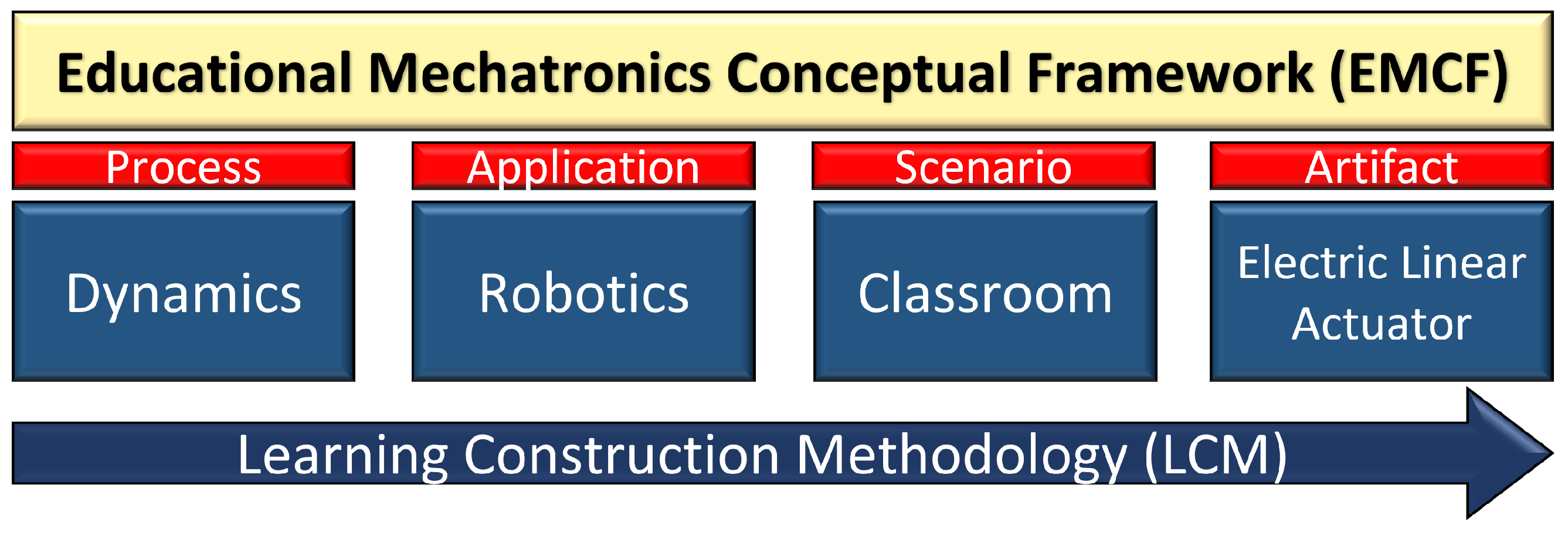
The EMCF aims to help learners understand abstract concepts that form the foundation of mechatronics applications through three reference perspectives: the process, the application, the scenario, and the artifacts. According to [
29], the first perspective covers the fundamental concepts of mechatronics as a process. The second perspective encompasses all sub-disciplines or applications derived from these concepts. The scenario perspective helps to place the application in context by considering the physical environment, which could be a laboratory or academic space or a virtual environment such as a remote laboratory or digital twin lab. Finally, the artifact perspective focuses on creating artifacts related to the process and application construction. This work implements the EMCF applied to an electric linear actuator to learn about uniform rectilinear motion.
Figure 1 shows the three reference perspectives of the EMCF applied to this specific proposal.
Moreover, this framework applies the learning construction methodology (EMCF-LCM). As presented in [
30], the EMCF-LCM proposes a three-level macro-process to construct a method of learning mechatronics concepts. It begins with the concrete level, which involves sensorimotor processes and manipulating and experimenting with objects (mechatronics artifacts). Next, it progresses to the graphic level, relating the elements of reality (the concrete level) with symbolic representations before concluding with the abstract learning level, which focuses on mathematical and formal concepts;
Figure 2 shows the three learning levels. This framework can help to establish a solid foundation in mechatronic thinking.
4. Electric Linear Actuator System
The electric linear actuator system was designed according to the EMCF and inspired by previous works [
29]. In this way, the linear actuator system acts as the mechatronic artifact, where three levels of EMCF-LCM are applied as described in
Figure 2. The system employs a USB camera placed 455 mm over the linear actuator to collect the position data and create an interactive learning experience for kinematics education. The complete system includes hardware such as the linear actuator, a tubular structure, and a graphical user interface developed in PyQt that employs computer vision, Python scripts, and an Arduino controller to interact with the actuator.
Figure 3 illustrates the proposed system architecture.
4.1. Electric Linear Actuator System Fabrication
The artifact depicted in
Figure 4 was designed according to the system architecture shown in
Figure 3. This section focuses on the procedure used to fabricate the system, which involved assembling the components, including the linear actuator, the tubular structure, and the camera support. These elements were designed using SolidWorks, a computer-aided design (CAD) software, and printed using Ultimaker Cura; these are both commonly used software worldwide.
The linear actuator employed a 12V DC motor with an embedded encoder providing rotational motion (see
Figure 5a). In order to convert rotational motion into linear motion, an 8 mm step lead screw was employed. The motor and the lead screw awee coupled using a 4.5 mm to 8 mm flexible coupling element. It is worth noting that no suitable commercial connection was identified. Therefore, the flexible coupling element was designed as shown in
Figure 5b and printed as shown in
Figure 5c. Finally,
Figure 5d shows the coupling of the lead screw and the motor using the flexible printed coupling.
As part of the linear actuator, the cart is a platform that moves along the rail and transports the load;
Figure 6a illustrates the designed cart. The cart was assembled with two linear shafts using the holes at extremes depicted in
Figure 6b and with the lead screw employing an anti-backlash nut, as depicted in
Figure 6c. Finally,
Figure 6d displays a top view of the cart with its load-stabilizing holes.
In order to provide support for the cart, motor, linear shafts, and lead screw, two limit supports were designed: the frontal support (see
Figure 7a) and the rear support (see
Figure 8a).
The frontal support was designed to assemble the DC motor, a limit switch, linear shafts, and the profile supports for the tubular structure described below. The printed frontal motor support is depicted in
Figure 7b,c, while
Figure 7d shows the motor mounting in the printed support. On the other hand, the printed rear support is depicted in
Figure 8b–d. Both pieces (
Figure 7 and
Figure 8) include slots for the assembly of the linear shaft elements and limit switch to restrict the cart’s movement and prevent it from exceeding the intended range. The assembly of the cart with the linear shafts, the lead screw, and the rear support is depicted in
Figure 9.
Two elements were printed for the tubular support;
Figure 10a,b shows the tubular printed supports designed to assemble the 30 × 30 aluminum profiles.
Figure 10c,d shows the assembled profiles with the linear actuator. Moreover, the two printed joints depicted in
Figure 11a,b were employed to assemble the aluminum profiles and to obtain the square shape. Finally, a camera housing support was created based on the size of the FIT0729 USB camera, as shown in
Figure 12a.
Figure 12b displays the housing support, which was shaped to allow for easy placement and rotation of the camera to achieve the desired position and angle. The assembly is depicted in
Figure 12c. Finally, Arduino and a l298n driver were employed to control the linear actuator’s DC motor, as depicted in
Figure 13.
4.2. Tracking and Localization Method Using Computer Vision Algorithms
In order to facilitate a comprehensive understanding of the uniform rectilinear motion concept, specifically as applied to the cart depicted in
Figure 6, it is necessary to determine its current position during travel. This work employs computer vision algorithms to measure the actual position of the cart in the linear actuator.
According to previous studies [
33], the architecture presented in
Figure 4 is suitable for implementing an indoor positioning system with a static camera (sensing device), elements, or features defined for detection (detected elements) via traditional image analysis (localization methods). The possible detectable elements of the cart are that it has the particularity of being a blue square; however, as previous works [
17,
29,
34,
35] indicate, employing a camera as a sensory tool for detecting features such as color proved challenging due to the need to keep consistent illumination levels throughout the process.
Other works employ artificial fiducial marks as detected elements to provide a point of reference for a measurement in an image. The fiducial markers used for localization and positioning are AprilTags, STag, ARTag, and ArUco markers; this last one shows a good position and orientation performance [
36]. ArUco offers a robust binary code that makes it resistant to errors, making error detection and a correction possible [
37]. ArUco has been employed in underwater visual navigation and a multi-sensor fusion indoor localization system for micro air vehicles and achieved accurate localization performance [
38,
39]. Therefore, ArUco markers have the potential to overcome the challenges of using cameras as sensors.
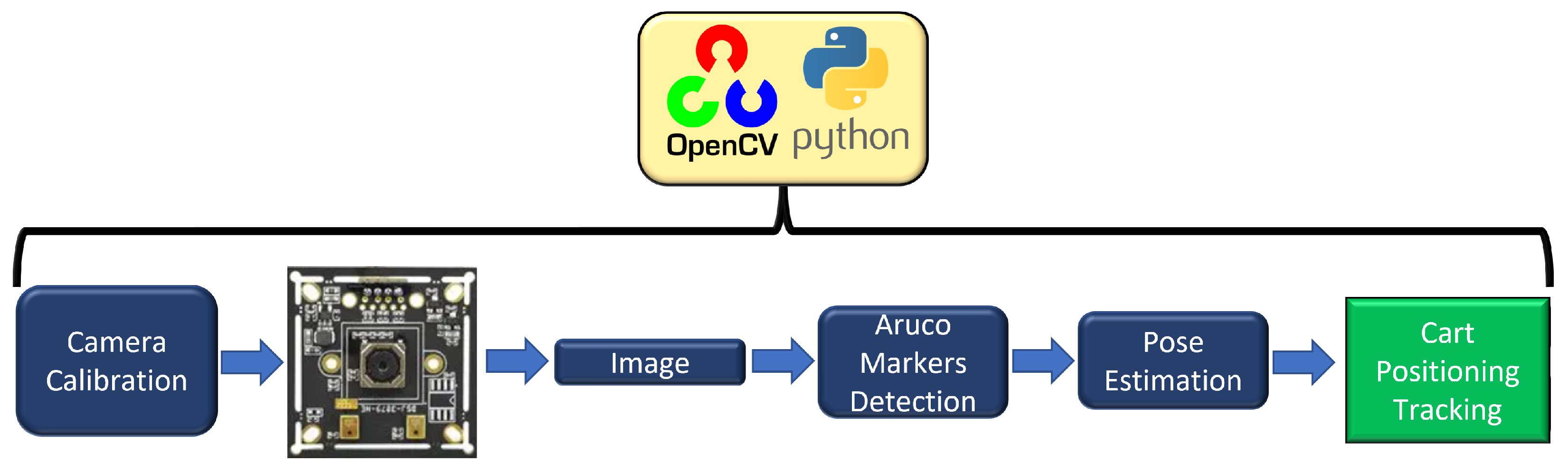
Thus, this work employs the pose estimation method by placing two ArUco markers strategically within the system. This process is based on finding correspondences between points in the real-world environment and their 2D image projection using fiducial marks (ArUco markers). The process of measuring the cart’s position using the OpenCV library in Python is depicted in
Figure 14. OpenCV is a powerful tool that offers efficient image processing and is widely used for real-time computer vision algorithms.
4.2.1. Camera Calibration
In order to accurately estimate the parameters of a camera lens, calibration is required due to the presence of two types of optical distortions: radial and tangential [
40]. The parameters for the calibration process can be calculated using methods described in prior research [
29]. As a result, the internal and external parameters of the camera are as follows:
The matrix
A contains the intrinsic parameters, including the focal elements
and
measured in pixels, as well as the coordinates of the main point, typically located at the center of the image, represented by
and
. Additionally, the vector
represents the distortion coefficients,
The data collected will be utilized in a subsequent phase of the image processing.
4.2.2. ArUco Marker Detection
The system employs a pair of independent 6 × 6 ArUco markers, each featuring a distinctive pattern and a binary-encoded ID, facilitating the individual estimation of the pose of each marker [
37]. The OpenCV library generates a pair of ArUco markers for the linear actuator with a square size of 26.5 mm, as depicted in
Figure 15. The markers are appropriately labeled with their respective IDs (one and two) to ensure efficient identification and tracking.
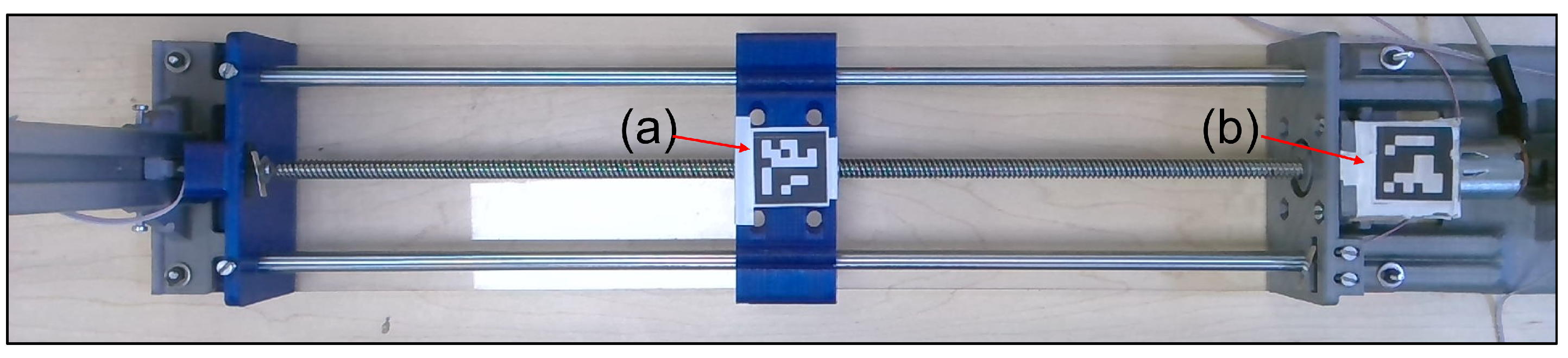
The ArUco marker with ID two is positioned on the cart to measure its current position; this ArUco marker is called the “cart marker”. In contrast, the ArUco marker with ID one operates as a reference point to calculate the precise location of the cart; this is called the “reference marker”.
Figure 16 shows the position of the ArUco markers.
A frame is obtained from the video capture and converted to grayscale. The result is introduced into the “detectmarkers()” function based on the works presented in [
37,
41]. This function lists the corners of the detected markers and their respective IDs. A square with the respective IDs is drawn in the detected elements. This process is depicted in
Figure 17.
4.2.3. Pose Estimation and Object Real-World Coordinates
The poses of the ArUco markers in the system are estimated by measuring their location relative to the camera’s position. This estimation is represented by a rotational and translational vector that extends from the camera lens to the center of the ArUco marker.
Figure 18 illustrates the pinhole camera model used in the system.
Converting a two-dimensional point denoted by the coordinates
to a three-dimensional point denoted by
involves employing Equation (
2).
where
A is the matrix of intrinsic parameters defined in Equation (
1), while
R and
T symbolize the rotation and translation of the camera, respectively.
In order to obtain the
R and
T vectors, it is necessary to collect three-dimensional (3D) position data from the four corners of the ArUco markers; this can be accomplished using the solvePnP algorithm in OpenCV, which employs the n-point projection method to derive rotation and translation matrices [
41,
42]. This method allows unknown values to be determined and represented as vectors, indicating the 3D position of the ArUco marker regarding the camera [
43]. The diagram in
Figure 19 presents the pose estimation and the coordinates of the ArUco markers.
The x and y coordinates (red font) are the coordinates of each ArUco marker with respect to the camera coordinates (0,0,0). Three axes are drawn in the center of the markers; red corresponds to the x axis, green corresponds to the y axis, and blue corresponds to the z axis. It is worth noting that the z and y axes are considered irrelevant due to the linear movement occurring only along the x axis.
4.2.4. Positioning Tracking
Upon completing pose estimation on the two markers, Equation (
3) can be employed to ascertain the precise positioning of the cart with respect to the reference marker.
Equation (
3) calculates the current position of the cart (
d) by finding the difference between the
x-axis coordinates of ArUco markers, represented by
and
, regarding the camera’s position. Additionally, a distance of 230 mm is subtracted from the result to establish the starting point as the midpoint of the cart’s travel. This distance represents the spatial separation between the center of the ArUco reference marker and the middle of the car’s travel along the linear actuator. As a result, the cart’s movement ranges from −180 to 180 mm, accounting for the cart’s width of 30 mm. This relationship is illustrated in
Figure 18. Then, a low-pass filter is employed.
Low-pass filters are commonly used in signal processing to smooth out abrupt value changes and reduce noise. In this sense, a low-pass filter is implemented to smooth the position value by taking a weighted average of the current and previous values using an exponential moving average, allowing us to produce more stable and consistent output. According to [
44], this specific type of filter can be customized through adjustable parameters, increasing its versatility for use in various applications. Equation (
4) describes a first-order low-pass filter.
where
represents the output value at time
n,
represents the input value at time
n, and
represents the output value at time
. The parameter
is a coefficient that determines the filter’s cutoff frequency. The camera rate is 30 frames per second, with a sampling time of 33 milliseconds. The resolution of the camera’s image is defined as 1920 × 1080. The tracking positioning process is described in Algorithm 1.
| Algorithm 1: Estimate of ArUco marker positions and calculated distance between two markers with filtering. |
- Require:
, , , , - Ensure:
- 1:
# Filter time constant (in seconds) - 2:
- 3:
# Sampling frequency (in Hz) - 4:
- 5:
# Filter coefficient - 6:
- 7:
# Initialization of filtered value - 8:
- 9:
if
is not empty then - 10:
Estimate the rotation and translation vectors for each detected marker using - 11:
for each detected marker do - 12:
if the marker ID is 1 or 2 then - 13:
Store the marker position in - 14:
end if - 15:
end for - 16:
end if - 17:
if contains both markers 1 and 2 then - 18:
Calculate the distance between the two markers as the absolute difference of their x-coordinates minus 230 mm - 19:
- 20:
- 21:
end if
|
4.3. Fuzzy Control
This work incorporates closed-loop and open-loop control strategies for instructional purposes. Specifically, a fuzzy controller is employed for the closed-loop control approach.
Figure 20 illustrates the block diagram of the fuzzy controller applied to the linear actuator.
The fuzzy controller performs four main steps: fuzzification, membership function selection, rules, and defuzzification [
45]:
First, during the fuzzification stage, the input information is transformed into fuzzy sets using linguistic expressions to convert fuzzy values.
In the inference process, the controller’s output is determined by establishing rules about linguistic variables; these rules are developed based on the placement of the linear actuator from input to output.
Within the system, the fuzzy controller’s input is determined by the difference between the desired and actual positions, while the voltage represents the output. The rules and membership functions are designed to ensure the controller is suitable. The rules for the input are defined as follows:
The rules for the output are defined as follows:
BNV: Big positive voltage;
SNV: Small negative voltage;
ZV: Zero voltage;
SPV: Small positive voltage;
BPV: Big positive voltage.
Finally, IF-THEN rules are employed as described in
Table 1.
For the input variable Error’s membership function, the range is set from −19 to 19, and for the output Voltage membership function, the range is set from −12 to 12. The BNE, BPE, BNV, and BPV membership functions are trapezoidal, while the remaining membership functions are triangular, as depicted in
Figure 21.
Figure 22 shows the response curve that defines the output
computed by the fuzzy controller as a function of the input variable
.
4.4. Encoder Sensor
The DC motor depicted in
Figure 5 contains an encoder that employs Hall effect sensors to detect the rotation of the motor shaft. As the motor rotates, the sensors generate pulses that the Arduino microcontroller counts. By measuring the time between pulses and the number of pulses per revolution, it is possible to calculate the speed of the motor in revolutions per minute (RPM). The encoder is employed in this work for educational activities. Thus, students will compare the average velocity computed by measured positions vs. the velocity measured by the encoder.
4.5. User Interface System Software
The user interface shown in
Figure 23 was created using pyQt5 and integrated with OpenCV features to enhance the proposed educational framework. pyQt5 is a popular library offering a wide range of design options and useful widgets, making it an optimal choice for creating desktop and mobile applications requiring a graphical user interface.
This software interface facilitates the capture of movements of the linear actuator and their conversion into concrete data. It also lets users control the linear actuator’s position using open- and closed-loop systems at a graphic level. Furthermore, data can be exported for analysis and calculations at an abstract level. The application also supports communication with the microcontroller via serial communication.
There are two ways to control the interface: open-loop and closed-loop control. With open-loop control, users can choose from three speeds (low, medium, and high) and control the direction of the motor with two buttons. Closed-loop mode automatically controls the cart’s position using a fuzzy controller. Users can set the target position and the increment for the target position.
Moreover, three graphs show the current position, the position vs. time, and the encoder speed data vs. time. By pressing the capture data button, the graphs will display the information. Additionally, all data can be downloaded in a comma separated values (CSV) format.
5. Instructional Design
This section describes the instructional design used to the mechatronic concept of rectilinear uniform motion. The instructional design is aligned with the EMCF, which involves three perspective entities: dynamics (process), robotics (application), and the classroom (scenario), as well as the linear actuator system (artifact). It consists of a hands-on learning practice for the EMCF levels, with the selected perspective developed in the subsequent subsections.
To conduct the practice, the student must initialize the user interface, and the linear actuator, by default, goes to the home position (). The system localizes the cart’s position by adding a yellow square indicating the actual position. Then, the practice can be conducted.
Practice: Rectilinear Motion in Open-Loop Control
This practice helps the student understand how a particle moving along a straight line is said to be in rectilinear motion. At any given instant t, the particle occupies a certain position on a straight line. The particle (cart) position is expressed in centimeters, and t is expressed in seconds. This way, the practice involves students determining the particle’s velocity over different motions and travel paths based on captured positional data.
At the concrete level, students use the linear actuator system interface to conduct hands-on learning experiments employing open-loop control. Through this process, they learn how to manipulate the actuator to produce varying speeds, as well as low, medium, and high voltage, and observe its corresponding motion behavior. Once students are familiarized with the interface, the set of instructions for the participants at the concrete level is as follows:
- 1.
Mark the “Low Voltage” checkbox to set the voltage to 2 volts. Then, move the linear actuator from its home position to the right direction by clicking once on “Start Motion to Right”, leaving the cart to reach the limit switch
mm as depicted in
Figure 24a.
- 2.
Press the “Capture Data” button on the user interface (see
Figure 24b), activating the capture of actual coordinates, the time when the capture data button was pressed, and the rpm of the motor. The graphs on the right side show the real-time data.
- 3.
Move the cart from its actual position to the left edge by clicking the “Start Motion to Left” button. Once the cart reaches the edge at 180 mm, click once more on the button “stop capture” to deactivate the capture of coordinates. Then, click on the “Export Position CSV” button; this generates a CSV file with the positional data vs. the time (see
Figure 24c).
At the graphic level, the student must relate the skills acquired at the concrete level with symbolic elements. In order to enhance students’ comprehension of the physical motion of the linear actuator, a CSV file with positioning data is generated, affording the visual illustration of the instructions at a tangible level. The objective is to encourage students to establish a correlation between a physical motion and its corresponding graphical representation. Thus, the instructions at the graphic level are as follows:
- 1.
The student opens the CSV file with recorded positioning data generated in previous instruction.
- 2.
The curve depicted in
Figure 25 is known as the motion curve. The motion curve represents the particle’s motion (
y axis) over time (
x axis). This way, the curve represents the cart’s linear motion from
mm to 180 mm performed at the concrete level.
- 3.
Now, a segment of the curve is selected, in this case a the interval of time from 6 s to 10 s is selected.
At the abstract level, the student relates the symbols assigned at the graphic level with the assistance of the instructor involving the rectilinear motion concept as follows.
In order to gain a better understanding of the movement of a particle, it is beneficial to examine its position at two distinct points in time:
t and
t +
. At time
t, the particle can be found at coordinate
. By introducing a small displacement
to the x-coordinate, the particle’s position at time
t +
can be determined. The particle’s left or right direction will dictate whether
is positive or negative. The particle’s average velocity over the time interval
can be computed as follows:
Figure 24.
Set of Instructions for concrete level: (a) concrete-level results of the 1st movement, (b) concrete-level results of the 2nd movement, (c) concrete-level results of the 3rd movement.
Figure 24.
Set of Instructions for concrete level: (a) concrete-level results of the 1st movement, (b) concrete-level results of the 2nd movement, (c) concrete-level results of the 3rd movement.
Figure 25.
Graphic level motion curve: Position vs. time data collected at the concrete level instructions, the red dashed lines represent the segment of the curve considered for the time intervals from 6 s to 10 s.
Figure 25.
Graphic level motion curve: Position vs. time data collected at the concrete level instructions, the red dashed lines represent the segment of the curve considered for the time intervals from 6 s to 10 s.
The data in
Figure 26 demonstrate a close correlation between the estimated average velocity and the measurements obtained through the encoder; this provides a means for students to verify the accuracy of their results and assess their performance as it pertains to the system’s measurements.
Therefore, in order to promote engagement in the learning process, students are instructed to calculate the velocity through the utilization of different speeds and shorter intervals of time.
6. Results
In assessing the performance of the linear actuator system, several key factors must be taken into account. These include the assessment of precision, which denotes the system’s ability to reproduce the same results consistently. The assessment of accuracy determines how closely the measured values match the actual values, and the resolution assessment quantifies the slightest detectable change in position that the system can respond to.
Additionally, the system’s rise time, settling time, and peak values are typically considered part of the fuzzy controller evaluation performance. The rise time refers to the duration it takes for a system to reach its intended position following a modification in the setpoint. Alternatively, the settling time is defined as the duration necessary for the system to stabilize and remain within a specific range around its steady-state value after a change in the setpoint. Furthermore, peak values indicate the maximum overshoot of the signal and demonstrate how far the system surpassed its target position before ultimately stabilizing.
Analyzing these parameters makes it feasible to evaluate the efficacy of the Linear Actuator system and pinpoint areas that necessitate enhancement.
6.1. System Accuracy and Precision Assessments
Therefore, to evaluate the system’s accuracy, we utilized a method of determining the absolute error by subtracting the measured position from the ground-truth position. In this way, three hundred pieces of position data were collected by each position from
mm to 180 mm. Subsequently, Equation (
7) was applied to calculate the mean absolute error (MAE). In this equation,
n represents the total number of position data points collected,
represents the measured position for the element at index
i, and
represents the actual (or ground-truth) position for the element at index
i. The result of this approach is depicted in
Figure 27.
In order to assess the precision of the system, the standard deviation was employed to measure the extent to which each measurement deviates from the actual values. Equation (
8) calculates the standard deviation, where
represents the standard deviation,
n represents the total number of data points,
represents the data point at index
i, and
represents the mean of all data points.
The standard deviation, calculated as the square root of the average of the squared differences between each data point and the norm, can be seen in
Figure 28.
According to the findings presented in
Figure 27, the maximum mean absolute (MAE) error in the current cart position is 2.5 mm, indicating an MAE position estimation of
mm. Additionally,
Figure 28, which assesses precision, demonstrates a maximum variability of 0.9 mm when the position x equals 100 mm. Finally,
Figure 29 depicts the position with the most significant variability. Moreover, the lighting fluctuations, the sampling rate, and the sudden changes in the cart’s position may contribute to the peaks obtained in the measurement data.
6.2. System Resolution Assessment
The sensor’s resolution represents the minimum detectable change in a physical quantity. This section describes the determination of the linear actuator system’s resolution.
The camera employed in this system has an image resolution of 1920 × 1080 pixels. Furthermore, the focal length (fx) can be derived from the intrinsic camera matrix presented in Equation (
1). This information enables us to calculate the horizontal angle field of view (hAFOV) and vertical angle field of view (vAFOV) employing Equations (
9) and (
10), where
and
are the width and the length of the camera’s image sensor in pixels.
The results can be utilized to determine the field of view for a predetermined distance of
cm, representing the camera’s height relative to the linear actuator. The horizontal and vertical field of view is calculated employing Equations (
11) and (
12), respectively.
Finally, the pixels per millimeter (PPmm) is used to determine the system resolution. The PPmm value defines the number of units of pixels for each meter of the projection image that the camera is capturing. Equations (
13) and (
14) are employed in this manner.
After conducting a resolution assessment, it was determined that the horizontal and vertical resolution values were px/mm. This resulted in a resolution measurement of mm suitable for the educational purpose of the system.
6.3. Fuzzy Controller Performance
To test the stability of the controller response, we evaluated its performance in set-point tracking. This test involves dividing the set point into two stages. The first stage ranges from
mm to 0 with a time interval of 0 s to 15 s, while the second stage ranges from 0 to 50 mm with a time interval of 20 s to 34 s. The results of this procedure are depicted in
Figure 30, while
Table 2 provides a comprehensive overview of the transient analysis of the response.
The performance of the linear actuator is presented in
Table 2. In the first stage, the controller achieved movement towards the target position in 2.62 s with a maximum overshoot of
mm. The settling time, which reflects the duration of the signal within a specific range around its steady-state value, was 14.5 s. In stage 2, a faster response time of 1.36 s was achieved, albeit with a more significant overshoot of
mm. The settling time was longer at 25.82 s when compared to stage 1. Upon evaluation, it can be ascertained that the system demonstrates commendable performance well-suited for educational purposes.
7. Discussion
This work describes the design, implementation, and control of our linear electric actuator system for educational purposes for teaching rectilinear particle motion in kinematics. The proposed tool was inspired by previous works in the field [
17,
26,
29], which employed vision-based control in their learning activities. In this way, the vision-based control method used in this work contributes to a comprehensive learning experience that melds theory, design, and practical implementation. An instructional design is presented based on the constructionist vision according to [
11], which differs from other approaches [
17,
18,
19,
21,
25] where a learning methodology was not defined. Moreover, in contrast to [
27,
28], this work integrates software and hardware to achieve a complete learning experience, providing a hands-on learning tool that addresses the gap between theory and practice, as evidenced in the literature [
46].
The proposed educational system was developed for implementation in the first semester of a robotics and mechatronics program, specifically for a “Introduction to Robotics and Mechatronics” course; for this case, fundamental physics and maths are required to perform the instructional practice. Although this concept may appear straightforward, it provides an essential foundation to comprehend more intricate kinematic principles.
The system employs a USB camera and a fuzzy position controller to enable an automated positioning control, all integrated into a user interface for interacting with the system. Although the encoder measurement might be a straightforward option for the proposed controller feedback, the incorporation of computer vision as controller feedback is due to the broader importance of this technology in modern mechatronic systems. Vision systems have become integral components in various engineering applications, from robotics to automation [
47]. Thus, we have implemented and reported a combination of fuzzy control and computer vision to bring a distinctive contribution to the engineering field.
The interface allows one to select between an open-loop controller and a closed-loop controller to perform different activities. In this study, one instructional design in the open loop was described. Accuracy, precision, resolution, and fuzzy controller performance are assessed to evaluate the system’s overall performance.
MAE and standard deviation are employed to evaluate the precision and accuracy, which show values of ± mm and mm, respectively, indicating that the system is reliable and produces consistent and precise results. In contrast, the system’s resolution indicates a value of mm, which is suitable for educational kinematics applications requiring precise measurements. The performance of the fuzzy controller was evaluated through set-point tracking tests. The system achieved a rise time of 2.62 s and 1.36 s for the test and settling times of 14.5 and 25.82 s at different tracking stages. The results show that the fuzzy controller provides the precise and accurate position of the linear actuator.
The results obtained in this evaluation support the suitability of the linear actuator system for use in educational applications in kinematics. However, some areas could be improved in future iterations of the system. Variations in lighting and sampling rates may significantly impact the results obtained. However, these challenges can be addressed by implementing image processing techniques and hardware enhancements, as discussed in other works [
17].
Traditional classroom demonstrations often rely on simplified models or animations, which can inadvertently oversimplify the real-world complexities students will encounter. The proposed system allows students to interact with a real-world mechanism that illustrates mechatronics concepts and their implications in more advanced scientific and engineering contexts. Although this work is an instructional guide for learning about a single concept in kinematics, the modular system design enables the modification of the overall interface to experience various learning concepts and their practical application in diverse contexts, such as control design.
Finally, a fuzzy position controller is used as the first evaluation experiment on the linear actuator. Further research will be conducted to investigate different control methods and offer students the opportunity to assess and contrast them in various educational settings, utilizing the same hands-on approach demonstrated in this current work.
Author Contributions
Conceptualization, L.F.L.-V., M.A.C.-M. and R.C.-N.; methodology, R.C.-N. and M.A.C.-M.; software, J.A.N.-P., M.E.M.-R. and S.C.-T.; validation, H.A.G.-O., L.F.L.-V., M.A.C.-M. and R.C.-N.; formal analysis, J.A.N.-P., L.E.G.-J. and M.E.M.-R.; investigation, J.A.N.-P., H.A.G.-O. and L.O.S.-S.; resources, M.A.C.-M. and R.C.-N.; data curation, J.A.N.-P.; writing—original draft preparation, J.A.N.-P. and L.F.L.-V.; writing—review and editing, L.F.L.-V., L.E.G.-J. and H.A.G.-O.; visualization, J.A.N.-P., S.C.-T. and H.A.G.-O.; supervision, L.F.L.-V., M.A.C.-M. and R.C.-N.; project administration, H.A.G.-O. and L.E.G.-J.; funding acquisition, M.A.C.-M., L.O.S.-S. and R.C.-N. All authors have read and agreed to the published version of the manuscript.
Funding
This research received no external funding.
Institutional Review Board Statement
Not applicable.
Informed Consent Statement
Not applicable.
Data Availability Statement
Not applicable.
Acknowledgments
The authors want to thank the Mexican National Council of Science and Technology CONACYT for its support to the National Laboratory of Embedded Systems, Advanced Electronics Design and Micro Systems (LN-SEDEAM by its initials in Spanish), projects number 282357, 293384, 299061, 314841, 315947, and 321128, as well as for scholarship 805876.
Conflicts of Interest
The authors declare no conflict of interest.
Abbreviations
The following abbreviations are used in this manuscript:
| ME | Mechanical engineering |
| EE | Electronic engineering |
| IT | Information technology |
| CS | Control system |
| STEM | Science, technology, engineering, and mathematics |
| CV | Computer vision |
| EMCF | Educational mechatronics conceptual framework |
| COTS | Commercial off-the-shelf |
| BPS | Ball–plate system |
| USB HD | Universal serial bus high definition |
| DC | Direct current |
| HVS | Hue saturation value |
| PID | Proportional integral derivative |
| EMCF-LCM | EMCF learning construction methodology |
| CAD | Computer-aided design |
| 3D | Three-dimensional |
| BNE | Big negative error |
| SNE | Small negative error |
| ZE | Zero error |
| SPE | Small positive error |
| BPE | Big positive error |
| BNV | Big negative voltage |
| SNV | Small negative voltage |
| ZV | Zero voltage |
| SPV | Small positive voltage |
| BPV | Big positive voltage |
| RPM | Revolutions per minute |
| CSV | Comma separated values |
| MAE | Mean absolute error |
| hAFOV | Horizontal angle field of view |
| vAFOV | Vertical angle field of view |
| PPM | Pixels per meter |
References
- Masayoshi, T. Mechatronics: From the 20th to 21st century. Control Eng. Pract. 2002, 10, 877–886. [Google Scholar]
- Filipescu, A.; Mincă, E.; Filipescu, A.; Coandă, H. Manufacturing Technology on a Mechatronics Line Assisted by Autonomous Robotic Systems, Robotic Manipulators and Visual Servoing Systems. Actuator 2020, 9, 127. [Google Scholar] [CrossRef]
- Cornejo, J.; Perales-Villarroel, J.P.; Sebastian, R.; Cornejo-Aguilar, J.A. Conceptual Design of Space Biosurgeon for Robotic Surgery and Aerospace Medicine. In Proceedings of the 2020 IEEE ANDESCON, Quito, Ecuador, 13 October 2020. [Google Scholar]
- Annaswamy, A.M.; Johansson, K.H.; Pappas, G.J. (Eds.) Control for Societal-Scale Challenges: Road Map 2030; IEEE Control Systems Society Publication: Piscataway, NJ, USA, 2023. [Google Scholar]
- Ma, J.; Li, X.; Tan, K.K. Advanced Optimization for Motion Control Systems; CRC Press: Boca Raton, FL, USA, 2020. [Google Scholar]
- Ceccarelli, M.; Ottaviano, E.; Carbone, G. A Role of Mechanical Engineering in Mechatronics. IFAC Proc. Vol. 2006, 39, 29–34. [Google Scholar]
- Craig, K.; Stolfi, F. Teaching control system design through mechatronics: Academic and industrial perspectives. Mechatronics 2002, 12, 371–381. [Google Scholar] [CrossRef]
- Habib, M.K.; Nagata, F.; Watanabe, K. Mechatronics: Experiential Learning and the Stimulation of Thinking Skills. Educ. Sci. 2021, 11, 46. [Google Scholar] [CrossRef]
- Boon Ng, S. Exploring STEM competences for the 21st century. In Current and Critical Issues in Curriculum, Learning and Assessment; UNESCO: Ginebra, Switzerland, 2019. [Google Scholar]
- Li, Y.; Schoenfeld, A.H.; diSessa, A.A. Design and Design Thinking in STEM Education. J. STEM Educ. Res. 2019, 2, 93–104. [Google Scholar] [CrossRef]
- Harel, I.; Papert, S. Software Design as a Learning Environment. Interact. Learn. Environ. 1990, 1, 1–32. [Google Scholar] [CrossRef]
- Haidar, A.; Al-Mutairi, M.; Al-Mutairi, A.; Al-Mutairi, F. Fuzzy Model Reference Adaptive Controller for Position Control of a DC Linear Actuator Motor in a Robotic Vehicle Driver. Int. J. Integr. Eng. 2020, 12, 235–244. [Google Scholar]
- Tawk, C.; Spinks, G.M.; in Het Panhuis, M.; Alici, G. 3D Printable Vacuum-Powered Soft Linear Actuators. In Proceedings of the 2019 IEEE/ASME International Conference on Advanced Intelligent Mechatronics (AIM), Hong Kong, China, 8–12 July 2019; pp. 50–55.
- Cui, L.; Phan, A.; Allison, G. Design and fabrication of a three dimensional printable non-assembly articulated hand exoskeleton for rehabilitation. In Proceedings of the 2015 37th Annual International Conference of the IEEE Engineering in Medicine and Biology Society (EMBC), Milan, Italy, 25–29 August 2015; pp. 4627–4630. [Google Scholar]
- Schmidt, M.; Kühnlenz, F.; Rinderknecht, S. Dynamic model predictive position control for linear actuators in automotive applications. In Proceedings of the 2018 Thirteenth International Conference on Ecological Vehicles and Renewable Energies (EVER), Monte-Carlo, Monaco, 10–12 April 2018; pp. 1–6. [Google Scholar]
- Sanfilippo, F.; Økter, M.; Eie, T.; Ottestad, M. Teaching Motion Control in Mechatronics Education Using an Open Framework Based on the Elevator Model. Machines 2022, 10, 945. [Google Scholar] [CrossRef]
- Tudić, V.; Kralj, D.; Hoster, J.; Tropčić, T. Design and Implementation of a Ball-Plate Control System and Python Script for Educational Purposes in STEM Technologies. Sensors 2022, 22, 1875. [Google Scholar] [CrossRef]
- Zhou, L.; Yoon, J.Y.; Andriën, A.; Nejad, M.I.; Allison, B.T.; Trumper, D.L. FlexLab and LevLab: A Portable Control and Mechatronics Educational System. IEEE/ASME Trans. Mechatron. 2020, 25, 305–315. [Google Scholar] [CrossRef]
- Bakaráč, P.; Kalúz, M.; Čirka, L. Design and development of a low-cost inverted pendulum for control education. In Proceedings of the 2017 21st International Conference on Process Control (PC), Strbske Pleso, Slovakia, 6–9 June 2017; pp. 398–403. [Google Scholar]
- Odry, Á.; Fullér, R.; Rudas, I.; Odry, P. Fuzzy control of self-balancing robots: A control laboratory project. Comput. Appl. Eng. Educ. 2020, 28, 512–535. [Google Scholar] [CrossRef]
- Takács, G.; Konkoly, T.; Gulan, M. OptoShield: A Low-Cost Tool for Control and Mechatronics Education. In Proceedings of the 2019 12th Asian Control Conference (ASCC), Kitakyushu, Japan, 9–12 June 2019; pp. 1001–1006. [Google Scholar]
- Aviles, M.; Rodríguez-Reséndiz, J.; Pérez-Ospina, J.; Lara-Mendoza, O. A Comprehensive Methodology for the Development of an Open Source Experimental Platform for Control Courses. Technologies 2023, 11, 25. [Google Scholar] [CrossRef]
- Torres-Salinas, H.; Rodríguez-Reséndiz, J.; Estévez-Bén, A.A.; Cruz Pérez, M.A.; Sevilla-Camacho, P.Y.; Perez-Soto, G.I. A Hands-On Laboratory for Intelligent Control Courses. Appl. Sci. 2020, 10, 9070. [Google Scholar] [CrossRef]
- Peters, A.A.; Vargas, F.J.; Garrido, C.; Andrade, C.; Villenas, F. PL-TOON: A Low-Cost Experimental Platform for Teaching and Research on Decentralized Cooperative Control. Sensors 2021, 21, 2072. [Google Scholar] [CrossRef]
- Assis, W.O.; Coelho, A.D. Use of Educational Tool for Modeling Temperature Control Systems as a Remote Teaching and Learning Strategy in Engineering. Int. J. Appl. Math. 2023, 53, 21. [Google Scholar]
- Rios, M.L.; Netto, J.F.d.M.; Almeida, T.O. Computational vision applied to the monitoring of mobile robots in educational robotic scenarios. In Proceedings of the 2017 IEEE Frontiers in Education Conference (FIE), Indianapolis, IN, USA, 18–21 October 2017. [Google Scholar]
- Aktaş, M.; Çavuş, B. A computer-aided educational tool for vector control of AC motors in graduate courses. Comput. Appl. Eng. Educ. 2020, 28, 705–723. [Google Scholar] [CrossRef]
- Muhiuddin, G.; Aguilera-Alvarez, J.; Padilla-Medina, J.; Martínez-Nolasco, C.; Samano-Ortega, V.; Bravo-Sanchez, M.; Martínez-Nolasco, J. Development of a Didactic Educational Tool for Learning Fuzzy Control Systems. Math. Probl. Eng. 2021, 2021, 3158342. [Google Scholar]
- Guerrero-Osuna, H.A.; Nava-Pintor, J.A.; Olvera-Olvera, C.A.; Ibarra-Pérez, T.; Carrasco-Navarro, R.; Luque-Vega, L.F. Educational Mechatronics Training System Based on Computer Vision for Mobile Robots. Sustainability 2023, 15, 1386. [Google Scholar] [CrossRef]
- Luque-Vega, L.F.; Lopez-Neri, E.; Arellano-Muro, C.A.; González-Jiménez, L.E.; Ghommam, J.; Saad, M.; Carrasco-Navarro, R.; Ruíz-Cruz, R.; Guerrero-Osuna, H.A. UAV-Based Smart Educational Mechatronics System Using a MoCap Laboratory and Hardware-in-the-Loop. Sensors 2022, 22, 5707. [Google Scholar] [CrossRef]
- Guerrero-Osuna, H.A.; Luque-Vega, L.F.; Carlos-Mancilla, M.A.; Ornelas-Vargas, G.; Castañeda-Miranda, V.H.; Carrasco-Navarro, R. Implementation of a MEIoT Weather Station with Exogenous Disturbance Input. Sensors 2021, 21, 1653. [Google Scholar] [CrossRef] [PubMed]
- Castañeda-Miranda, V.H.; Luque-Vega, L.F.; Lopez-Neri, E.; Nava-Pintor, J.A.; Guerrero-Osuna, H.A.; Ornelas-Vargas, G. Two-Dimensional Cartesian Coordinate System Educational Toolkit: 2D-CACSET. Sensors 2021, 21, 6304. [Google Scholar] [CrossRef]
- Morar, A.; Moldoveanu, A.; Mocanu, I.; Moldoveanu, F.; Radoi, I.E.; Asavei, V.; Gradinaru, A.; Butean, A. A Comprehensive Survey of Indoor Localization Methods Based on Computer Vision. Sensors 2020, 20, 2641. [Google Scholar] [CrossRef] [PubMed]
- Choi, H.-H. CVCC Model: Learning-Based Computer Vision Color Constancy with RiR-DSN Architecture. Sensors 2023, 23, 5341. [Google Scholar] [CrossRef] [PubMed]
- Wu, J.; Shen, T.; Wang, Q.; Tao, Z.; Zeng, K.; Song, J. Local Adaptive Illumination-Driven Input-Level Fusion for Infrared and Visible Object Detection. Remote Sens. 2023, 15, 660. [Google Scholar] [CrossRef]
- Kalaitzakis, M.; Cain, B.; Carroll, S.; Ambrosi, A.; Whitehead, C.; Vitzilaios, N. Fiducial Markers for Pose Estimation: Overview, Applications and Experimental Comparison of the ARTag, AprilTag, ArUco and STag Markers. J. Intell. Robot Syst. 2021, 101, 71. [Google Scholar] [CrossRef]
- OpenCV. Detection of ArUco Markers. Available online: https://docs.opencv.org/4.x/d5/dae/tutorial_aruco_detection.html (accessed on 24 June 2023).
- Xu, Z.; Haroutunian, M.; Murphy, A.J.; Neasham, J.; Norman, R. An Underwater Visual Navigation Method Based on Multiple ArUco Markers. J. Mar. Sci. Eng. 2021, 9, 1432. [Google Scholar] [CrossRef]
- Xing, B.; Zhu, Q.; Pan, F.; Feng, X. Marker-Based Multi-Sensor Fusion Indoor Localization System for Micro Air Vehicles. Sensors 2018, 18, 1706. [Google Scholar] [CrossRef]
- Sivkov, S.; Novikov, L.; Romanova, G.; Romanova, A.; Vaganov, D.; Valitov, M.; Vasiliev, S. The algorithm development for operation of a computer vision system via the OpenCV library. Procedia Comput. Sci. 2020, 169, 662–667. [Google Scholar] [CrossRef]
- Garrido-Jurado, S.; Muñoz-Salinas, R.; Madrid-Cuevas, F.J.; Marín-Jiménez, M.J. Automatic generation and detection of highly reliable fiducial markers under occlusion. Pattern Recognit. 2014, 47, 2280–2292. [Google Scholar] [CrossRef]
- Chen, C.-S.; Chang, W.-Y. Pose estimation for generalized imaging device via solving non-perspective N point problem. In Proceedings of the 2002 IEEE International Conference on Robotics and Automation (Cat. No.02CH37292), Washington, DC, USA, 11–15 May 2002; Volume 3, pp. 2931–2937. [Google Scholar]
- Guo, J.; Wu, P.; Wang, W. A precision pose measurement technique based on multi-cooperative logo. J. Phys. Conf. Ser. 2020, 1607, 0120471. [Google Scholar] [CrossRef]
- Petráš, I. Novel Generalized Low-Pass Filter with Adjustable Parameters of Exponential-Type Forgetting and Its Application to ECG Signal. Sensors 2022, 22, 8740. [Google Scholar] [CrossRef] [PubMed]
- Ross, T.J. Membership Functions, Fuzzification and Defuzzification. In Fuzzy Systems in Medicine; Szczepaniak, P.S., Lisboa, P.J.G., Kacprzyk, J., Eds.; Physica-Verlag HD: Heidelberg, Germany, 2000; pp. 69–86. [Google Scholar]
- Čech, M.; Königsmarková, J.; Goubej, M.; Oomen, T.; Visioli, A. Essential challenges in motion control education. IFAC-PapersOnLine 2019, 52, 200–205. [Google Scholar] [CrossRef]
- Okarma, K. Applications of Computer Vision in Automation and Robotics. Appl. Sci. 2020, 10, 6783. [Google Scholar] [CrossRef]
Figure 1.
The Educational Mechatronics Conceptual Framework (EMCF).
Figure 1.
The Educational Mechatronics Conceptual Framework (EMCF).
Figure 2.
Educational Mechatronics Conceptual Framework Learning Construction Methodology.
Figure 2.
Educational Mechatronics Conceptual Framework Learning Construction Methodology.
Figure 3.
Electric Linear Actuator System architecture comprised of a Linear Actuator, a tubular structure, a camera, and a user interface employing EMCF-LCM.
Figure 3.
Electric Linear Actuator System architecture comprised of a Linear Actuator, a tubular structure, a camera, and a user interface employing EMCF-LCM.
Figure 4.
Linear Actuator System Artifact.
Figure 4.
Linear Actuator System Artifact.
Figure 5.
Motor and lead screw coupling parts: (a) DC motor; (b) 4.5:8 mm Flexible coupling design; (c) printed flexible coupling; (d) coupling of the motor and the lead screw.
Figure 5.
Motor and lead screw coupling parts: (a) DC motor; (b) 4.5:8 mm Flexible coupling design; (c) printed flexible coupling; (d) coupling of the motor and the lead screw.
Figure 6.
Development of the cart: (a) cart design; (b) front-side view of printed cart; (c) rear-side view of printed cart; (d) top-side view of printed cart.
Figure 6.
Development of the cart: (a) cart design; (b) front-side view of printed cart; (c) rear-side view of printed cart; (d) top-side view of printed cart.
Figure 7.
DC motor support: (a) DC motor support design; (b) front view of the printed support; (c) rear view of the printed support; (d) motor mounting.
Figure 7.
DC motor support: (a) DC motor support design; (b) front view of the printed support; (c) rear view of the printed support; (d) motor mounting.
Figure 8.
Rear support: (a) rear support design; (b) front view of the printed support; (c) rear view of the printed support; (d) isometric view of the printed support.
Figure 8.
Rear support: (a) rear support design; (b) front view of the printed support; (c) rear view of the printed support; (d) isometric view of the printed support.
Figure 9.
Cart assembly: (a) assembly of the cart on the lead screw; (b) assembly of the cart with the linear shafts and lateral rear support.
Figure 9.
Cart assembly: (a) assembly of the cart on the lead screw; (b) assembly of the cart with the linear shafts and lateral rear support.
Figure 10.
Profile supports: (a) frontal profile support; (b) rear profile support; (c) frontal profile support assembly; (d) rear profile support assembly.
Figure 10.
Profile supports: (a) frontal profile support; (b) rear profile support; (c) frontal profile support assembly; (d) rear profile support assembly.
Figure 11.
Printed joints: (a) joint for corners and (b) joint for straight edges.
Figure 11.
Printed joints: (a) joint for corners and (b) joint for straight edges.
Figure 12.
Camera housing support: (a) USB FIT0729 camera; (b) printed housing; (c) assembled camera in housing support and aluminum profile.
Figure 12.
Camera housing support: (a) USB FIT0729 camera; (b) printed housing; (c) assembled camera in housing support and aluminum profile.
Figure 13.
Controllers: (a) Arduino Mega 2560 and (b) LN298n driver.
Figure 13.
Controllers: (a) Arduino Mega 2560 and (b) LN298n driver.
Figure 14.
Localization and tracking procedure stages.
Figure 14.
Localization and tracking procedure stages.
Figure 15.
Developed ArUco Markers: (a) reference marker and (b) cart marker.
Figure 15.
Developed ArUco Markers: (a) reference marker and (b) cart marker.
Figure 16.
ArUco markers: (a) ArUco marker with ID 2 on the cart and (b) reference ArUco with ID 1.
Figure 16.
ArUco markers: (a) ArUco marker with ID 2 on the cart and (b) reference ArUco with ID 1.
Figure 17.
ArUco marker detection process: (a) frame from video; (b) converting the frame to grayscale; (c) applying the detectmarkers() function; and (d) providing the list of corners and IDs.
Figure 17.
ArUco marker detection process: (a) frame from video; (b) converting the frame to grayscale; (c) applying the detectmarkers() function; and (d) providing the list of corners and IDs.
Figure 18.
General geometric relationship in the system: pinhole camera model and linear actuator’s working area.
Figure 18.
General geometric relationship in the system: pinhole camera model and linear actuator’s working area.
Figure 19.
Pose estimation: the image depicts the x and y coordinates regarding the camera (0,0,0). Three axes are shown; red corresponds to the x axis, green corresponds to the y axis, and blue corresponds to the z axis.
Figure 19.
Pose estimation: the image depicts the x and y coordinates regarding the camera (0,0,0). Three axes are shown; red corresponds to the x axis, green corresponds to the y axis, and blue corresponds to the z axis.
Figure 20.
Block diagram of fuzzy controller applied to the Linear Actuator.
Figure 20.
Block diagram of fuzzy controller applied to the Linear Actuator.
Figure 21.
Fuzzy Membership Functions: (a) Input Membership Functions and (b) Output Membership Functions.
Figure 21.
Fuzzy Membership Functions: (a) Input Membership Functions and (b) Output Membership Functions.
Figure 22.
The input–output control curve produced by the fuzzy controller.
Figure 22.
The input–output control curve produced by the fuzzy controller.
Figure 23.
Linear Actuator System graphical user interface developed in pyQt5 displaying the cart’s measured position in the 2D-plane, and the position and velocity with respect to time.
Figure 23.
Linear Actuator System graphical user interface developed in pyQt5 displaying the cart’s measured position in the 2D-plane, and the position and velocity with respect to time.
Figure 26.
Abstract level: Estimated average speed, the blue line denotes the speed measured by the encoder, while red dashed lines illustrate the estimated average speed in the time intervals from 6 s to 10 s.
Figure 26.
Abstract level: Estimated average speed, the blue line denotes the speed measured by the encoder, while red dashed lines illustrate the estimated average speed in the time intervals from 6 s to 10 s.
Figure 27.
Linear Actuator System Accuracy assessment for the position measurements.
Figure 27.
Linear Actuator System Accuracy assessment for the position measurements.
Figure 28.
Linear Actuator System precision assessment and the standard deviation for each position.
Figure 28.
Linear Actuator System precision assessment and the standard deviation for each position.
Figure 29.
Box plot for the position with the most significant variability (x = 10).
Figure 29.
Box plot for the position with the most significant variability (x = 10).
Figure 30.
Set-point tracking response for stage 1 and stage 2.
Figure 30.
Set-point tracking response for stage 1 and stage 2.
Table 1.
Linear Actuator Rules membership function.
Table 1.
Linear Actuator Rules membership function.
| Error | Voltage |
|---|
| BNE | BNV |
| SNE | SNV |
| ZE | ZV |
| SPE | SPV |
| BPE | BPV |
Table 2.
Performance evaluation of set-point tracking for the linear actuator system’s position controller.
Table 2.
Performance evaluation of set-point tracking for the linear actuator system’s position controller.
| | Rise Time (s) | Peak Value (mm) | Settling Time (s) |
|---|
| Stage 1 | 2.62 | 2.3 | 14.5 |
| Stage 2 | 1.36 | 52.6 | 25.82 |
| Disclaimer/Publisher’s Note: The statements, opinions and data contained in all publications are solely those of the individual author(s) and contributor(s) and not of MDPI and/or the editor(s). MDPI and/or the editor(s) disclaim responsibility for any injury to people or property resulting from any ideas, methods, instructions or products referred to in the content. |
© 2023 by the authors. Licensee MDPI, Basel, Switzerland. This article is an open access article distributed under the terms and conditions of the Creative Commons Attribution (CC BY) license (https://creativecommons.org/licenses/by/4.0/).


 ,
, 


