A Predictive Control Model of Bernoulli Production Line with Rework Loop for Real-Time WIP Optimization in Permutation Flowshop

Abstract

Permutation flowshop design and optimization are crucial in industry as they have a direct impact on production scheduling and efficiency. The ultimate goal is to model the production system (PSM) based on revealing the fundamental principles of the production process, and to schedule or reschedule production release plans in real time without interrupting work-in-progress (WIP). Most existing PSMs are focused on static production processes which fail to describe the dynamic relationships between machines and buffers. Therefore, this paper establishes a PSM to characterize both the static and transient behaviors of automatic and manual machines in the permutation flowshop manufacturing system. Building upon the established PSM, based on Bernoulli’s theory, discrete event model predictive control is proposed in this paper; its aim is to realize real-time optimization of production release plans without interfering with work-in-progress. According to the results of numerical examples, the discrete event model predictive control proposed in this paper is feasible and effective. The model established in this paper provides a theoretical basis for optimizing the effective operation of work-in-progress and replacement process systems.

1. Introduction

In traditional serial production systems, multiple machines are arranged consecutively, and the machines process tasks in sequence. This mode of production will be affected by dynamic events such as buffer starvation or blockage and machine stoppage [1]. To reduce the effects caused by uncertain events, the model of the permutation flowshop production line needs to consider two parts. The first is to model the production line; the second is to consider the rework production line. Specifically, on the main production line, the work is ongoing. The rework production line can reprocess or handle non-conforming work [2]. In such complex production systems, to enhance overall production efficiency and reduce the production cost, it is essential to optimize both operations and decision making in order to improve the performance of individual machines and systems. This production system is very complex, and in order to improve overall production efficiency, reduce production costs, and improve the performance of each machine and the entire system, it is necessary to optimize the operation and decision-making process. Permutation flowshop production lines have some unique characteristics, such as the low flexibility of some machines and buffers and the nonlinear correlation in the real-time capacity of the permutation flowshop, which pose critical challenges to effective, intelligent decision making [3].

Extensive investigations into permutation process problems and discrete event production systems have been conducted by scholars both on a domestic and international level, predominantly focusing on static production processes [4,5,6,7,8,9,10,11,12]. Chen et al. [4] utilized Markov analysis to scrutinize the production process within flexible production systems that handle multiple product types, rely on Bernoulli reliability model-compliant machines, and implement dedicated buffers. In an endeavor to minimize energy consumption, Yan et al. [5] meticulously analyzed the structural intricacies and conditions conducive to optimality in a two-machine Bernoulli serial production line. They derived two nonlinear algebraic equations characterizing these optimal conditions and introduced an efficacious binary search-based algorithm to solve said equations. Their work also includes a quantitative sensitivity analysis regarding how system parameters affect the optimal solution. Pei et al. [6] studied a series production line encompassing two Bernoulli machines, aiming to minimize total energy consumption whilst sustaining a specified production rate. Wang et al. [7] investigated on/off control strategies within a serial production line configuration compromised by unreliable machines and capacity-constrained buffers. Initially calculating strategies for lines with two or three machines, they subsequently adopted a decomposition technique to extrapolate these strategies to systems with a greater number of machines. Addressing the optimization problem of energy consumption in Bernoulli series production lines with more than two machines, Yan et al. [8] proposed a recursive methodology to enhance energy efficiency. In addition to these research trajectories, some scholars have amalgamated other cutting-edge technologies to expand investigation of these issues. Hadžić et al. [9] fused the benefits of finite state methods with genetic evolutionary algorithms to devise an innovative design technique, targeted at optimizing the lean design of Bernoulli series production lines. Subsequently, Hadžić et al. [10] utilized finite state methods to navigate the complexities associated with the assembly line production process, delivering a cost-effective computational mechanism to appraise assembly line performance in a steady state. Underpinning the need for precision and adaptability in simulation and modeling methods for discrete manufacturing workshops, Liu et al. [11] presented a logical modeling and simulation modality tailored to discrete manufacturing production processes. Tackling mixed-process scheduling challenges, Oztop et al. [12] developed a dual-objective mixed-integer linear programming model along with a unidirectional dual-objective constrained programming model. They further designed seven sophisticated dual-objective metaheuristic algorithms to address these complex scheduling dilemmas.

The above works in the literature only develop research on production problems from a steady-state perspective. When considering large-scale production operations, transient processes are often insignificant compared to the overall production duration, rendering steady-state analysis viable [13]. Nevertheless, in scenarios subject to frequent changes in orders and physical systems, such as in the manufacture of aircraft, ships, multi-variant furniture production plants, and the assembly lines for customized personal laptop computers, steady-state analysis may lack sufficient precision [14]. In order to solve this problem, some scholars have conducted relevant research on the transient process of the system. For example, Chen et al. [15] analyzed the dynamic behavior of a manufacturing system with regular orders and developed corresponding algorithms to make the modeling and estimation of the system solvable. Pagone et al. [16] conceptualized a framework for assessing manufacturing system robustness through intensive exploration of its structural and dynamic features. Mo et al. [17] introduced a paradigm that assimilates digital twins with modular artificial intelligence algorithms to dynamically reconfigure manufacturing systems to align with fluctuating consumer or market demands, addressing aspects such as layout, process parameters, and the scheduling of numerous assets. Wang et al. [18] defined the state expression function and reliability model of operator-based combined machine tools. Then, Bernoulli’s theory is used to calculate the state of the machine and buffer. Wang et al. [19] generated mathematical models and analytical solutions pertaining to single-machine and dual-machine production lines, proposing an efficient aggregation technique for lengthier production lines. Lastly, for systems bedeviled by product quality issues within a context of Bernoulli machines and Bernoulli quality inspection machines, Ma et al. [20] offered a Markov chain model of a dual-machine system to assess transient performance metrics.

The research of the above-mentioned articles focuses on the system analysis of flexible and discrete manufacturing. However, there is still insufficient research on complex replacement process manufacturing systems such as aircraft, ships, and computers. In the replacement process manufacturing system, the rework production line (i.e., entering the process) helps eliminate waste and reduce overall costs, as it effectively solves the problem of machine blockage and/or hunger. However, only a few analytical models have been established for permutation flowshop considering re-entrant links [21,22,23,24,25]. Furthermore, the mixed permutation flowshop consists of two types of machines: manual and automatic machines. Manual machines have a low degree of automation and require the machine operators to participate in production, whereas automatic machines do not need labor intervention. The probability of machine failure/success for automatic machines can be described by machine reliability, which can be evaluated by machine productivity. However, the reliability of manual machines cannot be assessed straightforwardly, because the potential human errors in machine tool selection and processing play a critical factor in machine reliability [26,27,28]. At present, scholars have conducted research on manufacturing processes containing rework loops. Producing defective products is a very common phenomenon. Bachar et al. [21] developed a flexible production model that can redesign repairable defecation products and outsource the products to prevent backlogs. As closed-loop production lines with a constant number of carriers are widely used, Zhou et al. [22] proposed a closed-loop production line production performance evaluation and optimization model considering the quality degradation level and rework process. In view of the problems faced by production systems that adopt the “immediate rework” mechanism, such as high complexity of equipment composition and long idling time of idle machines, SUN et al. [23] built a digital twin system for energy consumption optimization of production systems, integrating real-time data to achieve optimal caching based on online energy consumption optimization of zone thresholds. Considering unreliable machines and limited buffers, Jia et al. [24] studied the problem of dynamic process modeling and real-time performance evaluation of rework systems. By integrating resource allocation and rework decisions into the tolerance allocation problem, Khezri et al. [25] proposed a cost modeling method to minimize manufacturing costs in terms of resource allocation and rework decisions. In order to make the research more realistic, some scholars have conducted research on human factors in manufacturing systems. Chen et al. [26] evaluated automation or robot collaboration on an existing assembly line to help workers reduce repetitive tasks and increase productivity. Lago et al. [27] proposed a method to incorporate human factors into digital twins to provide recommendations on employee rotation based on their previous performance during the shift. Shi et al. [28] studied a new boredom-aware dual-resource-constrained flexible job shop scheduling problem and constructed an efficiency function to characterize the impact of worker boredom.

In summary, scholars have conducted a large number of extended studies on static and transient production processes which achieved curtained research results. However, the current literature on production system modeling has the following limitations:

(1)

Most current modeling efforts mainly focus on static production processes, and steady-state analysis is effective in the case of a single large-scale production. In complex and changeable streamlined production processes, compared with transient analysis, the results obtained by steady-state analysis are not accurate enough in some cases. However, the current transient modeling work on production systems is still insufficient.

(2)

The rework and reuse of defective products is of great significance to reducing costs, improving manufacturing efficiency, and realizing green manufacturing. Currently, the existing transient modeling work mainly focuses on continuous manufacturing systems, and it is difficult to consider complex re-entrant systems. There is still insufficient research on this link.

(3)

In the actual production process, human factors play a large role in the safety, risk management, and quality control of the production system. However, current research on the replacement process usually only considers automatic machines and does not consider manual machines that are affected by the human actions of the machine operator.

To address these limitations, this research proposes to establish a production line performance prediction model based upon the instantaneous state probability of the system to reflect the dynamic changes of the manufacturing system states in real time. This research aims to model the permutation flowshop with re-entrant links and conduct dynamic analysis to provide a solid foundation for optimizing the operations and enabling intelligent decision making. The main contributions of this paper are:

(1)

This paper presents an analysis of automated and manually operated semi-automated machines and their integration into a displacement flowshop with a rework loop.

(2)

This study establishes an instantaneous productivity model suitable for arranging flow operations with rework loops and human factors, and measures basic production performance indicators through a recursive method.

(3)

To address the challenges of intelligent control in permutation flowshops and to furnish comprehensive, real-time production insights, a model predictive control system based on discrete event-driven feedback is employed. As a result of these research outcomes, there is a discernible enhancement in the ability to perceive and predict work-in-progress, leading to significant savings in human resources.

The remaining chapters of this paper include the following sections. Section 2 introduces the problem description and model assumptions. Section 3 introduces the modeling of the production system for the replacement flowchart. Section 4 analyzes the algorithm for solving the established model. Section 5 conducts numerical case studies. Section 6 includes the research conclusions of this paper and future work.

2. Problem Description and Model Assumptions

The traditional serial production system has machines that are connected in a serial way, where a material storage device (or buffer) exists between the two machines to convey products from one machine to another. A traditional serial production line, with a rectangle representing M machines and a circle representing M-1 buffers, is shown in Figure 1. Hunger and congestion often occur on this serial production line [29].

A permutation process model with re-entrant links has been established which can solve the problem of traditional tandem production lines. Figure 2 shows that the main production line and rework production line constitute the production system. In this system, $m_{i,j}$ denotes the processing machine; $b_{i,j}$ denotes the buffer of storage and transportation equipment (AGV). Moreover, parameter i, i = 1, 2, 3, …, n, means the computer or buffer index. The parameter j means the index of production lines. The parameters n and r mean another index number of machines (n, r ≥ 2). Three main production lines include Line1 ($m_{1,1}\to m_{n,1}$), Line2 ($m_{1,2}\to m_{n,2}$), and Line3 ($m_{n+1,3}\to b_{n+2,3}$), which can provide processing of parts for the end product. Parts can be transferred by AGV on the main production line Line4 ($b_{n,4}\to m_{n+r+1,4}$) and Line5 ($b_{n,5}\to m_{n+r+1,5}$) are called rework production lines; they can assist in reprocessing non-conforming parts on the main production line. If the $m_{i,j}$ probability of being non-faulty at any time is $P_{i,j}$, then the probability of being faulty is $1-P_{i,j}$. At any given moment, since the probability of failure for all busy machines is considered independent, the occurrence of a failure in one busy machine does not affect the probability of failures in other busy machines. If the number of tool types on the machine $m_{i,j}$ is $T_{i,j}$, the number of parts to be processed is $A_{i,j}$, the $b_{i,j}$ maximum inventory level of is $Q_{i,j}$, and C is the number of buffers. It is assumed that each machine in the permutation flowshop can process the same number of parts per unit time. If the amount of parts processed by each machine at the same time is the same, to reduce the difficulty of calculation, the number of parts is assumed to be 1. The total processing time is evenly divided into several sections according to the number of machines. Assuming the total processing time is M, the initial moment is expressed as t = 0, the end of the first moment is represented as t = 1, and the last moment is represented as t = M [30].

Four hypotheses are used to model the transient production of a permutation flowshop with re-entrant links, described as follows.

(1)

There are M machines and M-1 buffers on the main production line. Among them, there are two rework production lines, on which is an inspection machine which can check whether the products are qualified. Qualified products are recorded as class A products, and unqualified products are recorded as class B products. Qualified products are directly transferred to the buffer, and unqualified products are sent for or wait for reprocessing through the rework production line [31].

(2)

At least one machine has sufficient raw materials, and the last machine on the production line of Line 3 will not be blocked [32].

(3)

The start time of each production determines the working status of the machine, and the end time of each production determines the status of the buffer [33].

(4)

The entire replacement process with re-entry satisfies the assumptions of “time dependent failure” and “pre-processing blocking” [34].

3. Production System Modeling and Predictive Model Control

3.1. Production System Modeling

3.1.1. Machine Reliability Model for Both Manual and Automatic Machines

In the permutation flowshop with re-entrant links, the specific indicators include Rework Rate (RR), Production Rate (PR), Energy-Consuming Reduction Rate (ECRA), etc. The reliability of automatic machines is determined when the parts and tools to be processed are determined, and the factors of human interference in the production process are very small [18]. Productivity is an important indicator of reliability characteristics. The number of parts to be processed and the selection of processing tools limit the reliability of manual machine tools. The number of parts and the correct choice of processing tools become the factors that interfere with reliability, so the reliability of the machine is jointly determined by the choice of processing personnel and process reliability. Based on the explanation of selection complexity [12], the selection equation of $T_{i,j}$ and $A_{i,j}$ for the operator of the machine $m_{i,j}$ can be expressed as follows.

$$\left\{\begin{array}{l}{H}_{i,j}^T=-{\displaystyle \sum _{x=1}^{T_{i,j}}{F}_x·{\log }_2{F}_x}\\ H_{i,j}^A=-{\displaystyle \sum _{x=1}^{A_{i,j}}{F}_y·{\log }_2{F}_y}\end{array}\right.$$

(1)

In Equation (1), $H_{i,j}^T$ is the probability of processing personnel in selecting tools at $m_{i,j}$; $H_{i,j}^A$ is the probability of $m_{i,j}$’s processing personnel for the parts to be processed. x is a random variable and it represents the choice of machining parts by the processing personnel. y is a random variable and it represents the choice of machining parts by the processing personnel. $F_x$ is the probability that the processing personnel selects x, and $F_y$ is the probability that the processing personnel selects y. When $F_x$ = 1 (or $F_y$ = 1), Equation (4) becomes 0, indicating that the choice of production tools and parts to be machined have been determined, and the random variable x (or y) has also been determined. According to the above equation and the current literature [15], it can be deduced that the average reaction time of $m_{i,j}$ to $T_{i,j}$ and $A_{i,j}$ is, respectively,

$$\left\{\begin{array}{l}R{T}_{i,j}^T={\alpha }^1+{\beta }^1·H_{i,j}^T\\ R{T}_{i,j}^A={\alpha }^2+{\beta }^2·H_{i,j}^A\end{array}\right.$$

(2)

In Equation (2), $R{T}_{i,j}^T$ is the average reaction time of the processing personnel selecting the correct processing tool in $m_{i,j}$. $R{T}_{i,j}^A$ is the average reaction time of the processing personnel in $m_{i,j}$ selecting the correct production parts; ${\alpha }^1,{\alpha }^2,{\beta }^1,{\beta }^2$ are constants. Therefore, the total average response time of the processing personnel to $T_{i,j}$ and $A_{i,j}$ in $m_{i,j}$ can be obtained by Equation (3).

$$R{T}_{i,j}=R{T}_{i,j}^T+R{T}_{i,j}^A$$

(3)

On the basis of the above equation, according to the research of Yang [21], the calculation equation of machine reliability is formulated as follows.

$$P_{i,j}={\omega }_{i,j}·{\mathcal{l}}^{-{[R{T}_{i,j}/{\eta }_{i,j}]}^{\gamma }}$$

(4)

In Equation (4), ${\omega }_{i,j}$ is the process reliability of $m_{i,j}$, ${\eta }_{i,j}$ is the scaling parameter of Weibull reliability function, and γ (γ > 1) is the risk rate of the Weibull reliability function. In Equations (3) and (4), when $H_{i,j}^T$ or $H_{i,j}^A$ is equal to 0, there is only one variable ${\omega }_{i,j}$, so the reliability of the machine only depends on ${\omega }_{i,j}$. When the number of $T_{i,j}$ or $A_{i,j}$ increases, the artificial reliability is inversely proportional to it, so it will decrease.

3.1.2. Transient Transition Modeling

To simplify the calculation of the state of each machine, the following operators and notations are introduced to describe some objects or events.

(1)

Operator P describes the probability of occurrence of event E (i.e., P[E]).

(2)

The operator Φ describes the event that the object O is in state S at time t, respectively, Φ (O, S, t).

(3)

The operator H describes multiple objects (O₁, O₂, O₃, …) At time t, they are in states (S₁, S₂, S₃, …), respectively, H (O₁, O₂, O₃, …/S₁, S₂, S₃, …, t)

(4)

The operator T describes the probability of a particular object O going from state S₁ to S₂ in time t, respectively, $T^{S_2,S_1}(t)$.

The following notations are used to describe the different operating states of the machine in a unit time period, as shown in

Table 1. Notations for different machine states.

Notation	Interpretation
$U{P}_{i,j}(t)$	The machine is in a state of non-fault operation in unit time t
$D{N}_{i,j}(t)$	A machine or buffer that is out of order within a time unit t
$P{R}_{i,j}(t)$	The operation of a machine within a time unit t
$NP{R}_{i,j}(t)$	The state in which a machine operates non-productively within a time unit t
$S{T}_{i,j}(t)$	The machine or buffer operates in a hungry state for a unit time t
$NS{T}_{i,j}(t)$	The machine or buffer unit is not hungry within unit time t
$B{L}_{i,j}(t)$	The operation of a machine or buffer that is blocked for a unit of time t
$NB{L}_{i,j}(t)$	The state of unblocked operation of a machine or buffer for a unit of time t
$\theta$	The complete set of all possible states of a machine
$X_{i,j}(t)$	Time instant at which the machine $m_{i,j}$ starts to work on the t-th part
$y(t)$	Time instant at which the t-th part leaves the permutation flowshop
${\sigma }_{i,j}(t)$	Processing time of the t-th part at $m_{i,j}$
$N_i^{-}\left(t\right)$	The buffer level after the t-th part’s entrance into $b_{i,j}$
$N_i^{+}\left(t\right)$	The buffer level of $b_{i,j}$ just after the t-th part leaves $b_{i,j}$
$N_c$	The control range of discrete event model predictive control
$N_p$	The prediction horizon of the discrete event model predictive control, Nc ≤ Np
$N_i$	The capacity of the buffer $b_{i,j}$
$r(t)$	The expiration date of the finished product
$u(t)$	The time when the t-th component is fed to the system
${\overrightarrow{\mathrm{e}}}_i=(\mathrm{j},t_i,{\mathrm{d}}_i)$	A disturbing event that lasts di time when the machine $m_{i,j}$ processes the t-th part

.

Based on different machine states, the logical relationships between the operating states of each machine in the permutation flowshop are shown in Figure 3.

As shown in Figure 3, the machine can be in a state of blockage and starvation at the same time. Furthermore, there can only be one running state at each moment, and the rest of the states are shown in Equation (5).

$$\left\{\begin{array}{l}\Phi (m_{i,j},\mathrm{P}{R}_{i,j},t)=\Phi (m_{i,j},U{P}_{i,j},t)\cap \Phi (m_{i,j},NS{T}_{i,j},t)\cap \Phi (m_{i,j},NB{L}_{i,j},t);\\ \Phi (m_{i,j},N\mathrm{P}{R}_{i,j},t)=\Phi (m_{i,j},D{N}_{i,j},t)\cup \Phi (m_{i,j},S{T}_{i,j},t)\cup \Phi (m_{i,j},B{L}_{i,j},t);\\ \Phi (m_{i,j},U{P}_{i,j},t)\cup \Phi (m_{i,j},D{N}_{i,j},t)=\theta ;\\ \Phi (m_{i,j},U{P}_{i,j},t)\cap \Phi (m_{i,j},D{N}_{i,j},t)=\varnothing ;\\ \Phi (m_{i,j},\mathrm{P}{R}_{i,j},t)\cap \Phi (m_{i,j},S{T}_{i,j},t)=\varnothing ;\\ \Phi (m_{i,j},\mathrm{P}{R}_{i,j},t)\cap \Phi (m_{i,j},B{L}_{i,j},t)=\varnothing .\end{array}\right.$$

(5)

The reason for the state change of the manufacturing system in the permutation flowshop is that each machine presents different running states at different times. Because there is no memory in every machine, the instantaneous occupancy of the buffer is used to describe the transient state of the system. To explain this process, three machine manufacturing systems (Line1 = Line2 = Line3) are taken as an example. There are three machines and three buffers on two main production lines of Line1 and Line2, and one test machine, two machines, and three buffers on Line3, and the set of their combined states is shown in

Table 2. The combined state sets for 3-machine-3-buffer permutation flowshop.

Type	${\mathit{m}}_{1,1}$	${\mathit{m}}_{2,1}$	${\mathit{m}}_{3,1}$
A	×	×	×
B	×	×	√
C	×	√	×
D	×	√	√
E	√	×	×
F	√	×	√
G	√	√	×
H	√	√	√

. It is assumed that α, β, and γ represent the immediate possession of the buffer $b_{1,1}$, $b_{2,1}$, $b_{3,1}$ ($\alpha ,\beta ,\gamma \in N,\alpha \le Q_{1,1},\beta \le Q_{2,1},\gamma \le Q_{3,1}$). At the beginning of production of the machine (i.e., at t = 0), the number of buffers $b_{1,1}$, $b_{2,1}$, $b_{3,1}$ is 0, so (000) represents the system’s state at t = 0. As the processing progresses, the state of each machine will change, and the number of buffers will also change. Now, assume that × means that the machine is in a fault state; √ indicates that the machine is in a non-fault state.

When the machine is at different running states at different times, the immediate occupancy of the buffer will change accordingly. For example, suppose that the immediate occupancy of the permutation flowshop is all 0 at time t = 0; the combined state of the machine is typing A (or B) in Table 1. System status at time t = 1 can only be (000). It can be seen that under the action of eight different types of machine combination states, the system can only be in one of the two states (000) and (100) at t = 1. Based on operator H and operator T, the transient transition relation of the permutation flowshop manufacturing system can be obtained by Equation (6).

$$P[H(b_1,b_2,b_3/k_1,k_2,k_3,t)]=\Gamma (P[H(b_1{b}_2{b}_3/k_1^{\prime },k_2^{\prime },k_3^{\prime },t-1)])$$

(6)

In Equation (6), $k_1,k_2,k_3$ represent the instantaneous occupancy of the buffer in the permutation flowshop at time t; $k_1^{\prime },k_2^{\prime },k_3^{\prime }$ represent the real-time occupancy of the buffer at time t − 1. $\Gamma ( )$ represents the mapping relationship between transient states of three machine manufacturing systems during the period from t − 1 to t, as shown in Figure 4.

3.1.3. Transient Mapping Analysis

In the production process of permutation flowshop with re-entrant links, for each machine, only one product is processed at a time and the number of buffers can only increase one product at a time, that is to say, the change of the immediate occupancy of each buffer can only appear as −1, 0, +1 in unit time. Based on the above analysis, the transient transition relation of buffer $b_{i,j}$ at time t is described with operator T, as shown in Figure 5.

If the buffer $b_{i,j}$ immediate possessiveness at time t is k ($k\ne 0, k\ne Q_{i,j}$), then the buffer $b_{i,j}$ immediate possessiveness at time t − 1 can only be k − 1, k, and k + 1. The corresponding state transition probability is, respectively: $T_{i,j}^{k,k-1}(t),T_{i,j}^{k,k}(t),T_{i,j}^{k,k+1}(t)$ [16]. Based on the above, the buffer $b_{i,j}$ at t time instant with the number zero probability can be expressed as the buffer occupancy of instant in t − 1 time for probability multiplied by the buffer occupancy of instant in time t, namely, the buffer occupancy at the time instant t − 1 and t is 0. Another possibility is that the buffer at time t is −1 to 1 in the number of real time. At time t, the immediate occupancy is reduced to 0 due to the downstream machine.

Assuming the direct occupancy of buffer $b_{i,j}$ at time t is 1, there exist the following four situations. The first situation is that the buffer $b_{i,j}$ at t − 1 moment of immediate occupancy is 0, due to the upstream machine processing; the product is transported to the buffer. Therefore, the direct occupancy of the buffer increases. Secondly, it is not possible to deal with the upstream or downstream side of the buffer $b_{i,j}$ because of failure or blockage, so the direct occupancy of the buffer remains unchanged at t − 1 and t, and remains 1. In the third situation, both upstream and downstream of the buffer $b_{i,j}$ can be processed normally, so that the immediate occupancy of the buffer $b_{i,j}$ does not have any change between time t − 1 and time t, remaining 1. In the last situation, the buffer $b_{i,j}$’s immediate occupancy is 2 at t − 1, because the downstream machine can carry out normal production, while the upstream buffer cannot transfer products due to faults and other reasons, so the buffer’s immediate occupancy becomes 1. The rest can be obtained by analogy. Therefore, according to the total probability equation, it can be obtained by Equation (7).

$$\left\{\begin{array}{l}P[\Phi (b_{i,j},0,t)]=T_{i,j}^{0,0}(t)·P[\Phi (b_{i,j},0,t-1)]+T_{i,j}^{0,1}(t)·P[\Phi (b_{i,j},1,t-1)]\hfill \\ P[\Phi (b_{i,j},1,t)]=T_{i,j}^{1,0}(t)·P[\Phi (b_{i,j},0,t-1)]+T_i^{1,1}(t)·P[\Phi (b_{i,j},1,t-1)]+T_{i,j}^{1,2}(t)·P[\Phi (b_{i,j},2,t-1)]\hfill \\ P[\Phi (b_{i,j},2,t)]=T_{i,j}^{2,1}(t)·P[\Phi (b_{i,j},1,t-1)]+T_{i,j}^{2,2}(t)·P[\Phi (b_{i,j},2,t-1)]+T_{i,j}^{2,3}(t)·P[\Phi (b_{i,j},3,t-1)]\hfill \\ \cdots \hfill \\ P[\Phi (b_{i,j},k,t)]=T_{i,j}^{k,k-1}(t)·P[\Phi (b_{i,j},k-1,t-1)]+T_{i,j}^{k,k}(t)·P[\Phi (b_{i,j},k,t-1)]\hfill \\ \hspace{1em}\hspace{1em}\hspace{1em}\hspace{1em}\hspace{1em} +T_{i,j}^{k,k+1}(t)·P[\Phi (b_{i,j},k+1,t-1)]\hfill \\ \cdots \hfill \\ P[\Phi (b_{i,j},Q_{i,j}-1,t)]=T_{i,j}^{Q_{i,j}-1,Q_{i,j}}(t)·P[\Phi (b_{i,j},Q_{i,j},t-1)]+T_{i,j}^{Q_{i,j}-1,Q_{i,j}-1}(t)·P[\Phi (b_{i,j},Q_{i,j}-1,t-1)]\hfill \\ \hspace{1em}\hspace{1em}\hspace{1em}\hspace{1em}\hspace{1em}\hspace{1em}\hspace{1em}+T_{i,j}^{Q_{i,j}-1,Q_{i,j}-2}(t)·P[\Phi (b_{i,j},Q_{i,j}-2,t-1)]\hfill \\ P[\Phi (b_{i,j},Q_{i,j},t)]=T_{i,j}^{Q_{i,j},Q_{i,j}-1}(t)·P[\Phi (b_{i,j},Q_{i,j}-1,t-1)]+T_{i,j}^{Q_{i,j},Q_{i,j}}(t)·P[\Phi (b_{i,j},Q_{i,j},t-1)]\hfill \end{array}\right.$$

(7)

In the last expression, there are only two situations; since $b_{i,j}$ is the maximum inventory level of the buffer, there is no situation of $Q_{i,j}$ + 1. The above equation can only be established under the premise of Equation (8); the total probability of all possibilities of the immediate occupancy of buffer $b_{i,j}$ at time t is 1, as shown in Equation (8).

$${\displaystyle \sum _{u=1}^{Q_{i,j}}P[\Phi (b_{i,j},u,t)]=1}$$

(8)

The matrix expression of Equation (8) is shown in Equation (9).

$$\left[\begin{array}{c}P[\Phi (b_{i,j},0,t)]\\ ⋮\\ P[\Phi (b_{i,j},Q_{i,j},t)]\end{array}\right]=\left[\begin{array}{cccc}{T}_{i,j}^{0,0}(t)& T_{i,j}^{0,1}(t)& 0& \cdots \\ \cdots & & & \cdots \\ \cdots & T_{i,j}^{k,k-1}(t)& T_{i,j}^{k,k}(t)& T_{i,j}^{k,k+1}(t)\\ \cdots & & & \cdots \\ \cdots & 0& T_{i,j}^{Q_{i,j}}(t)& T_{i,j}^{Q_{i+1,j}}(t)\end{array}\right].\left[\begin{array}{c}P[\Phi (b_{i,j},0,t-1)]\\ \cdots \\ P[\Phi (b_{i,j},k,t-1)]\\ \cdots \\ P[\Phi (b_{i,j},Q_{i,j},t-1)]\end{array}\right]$$

(9)

3.1.4. Reverse Modeling of Machine Transient Behavior

In the arrangement process, the transient state of the system during the production process may change due to the different operating states of each machine. On this basis, this paper conducts reverse modeling to solve the transition probability. In fact, the state of the machines connected to each buffer in the permutation flowchart determines the current change in occupancy rate. For example, when the immediate occupancy of the buffer $b_{i,j}$ is k at t − 1 and k + 1 at t, the state of $m_{i,j}$ must be $P{R}_{i,j}(t)$; the state of $m_{i+1,j}$ must be $NP{R}_{i,j}(t)$ during the unit period from t − 1 to t. Similarly, when the immediate occupancy of the buffer $b_{i,j}$ is k + 1 at t − 1 and k at t, $m_{i,j}$ must be $NP{R}_{i,j}(t)$; $m_{i+1,j}$ must be $P{R}_{i,j}(t)$ in the unit time from t − 1 to t. When the immediate occupancy of the buffer $b_{i,j}$ is k at both t − 1 and t, $m_{i,j}$ and $m_{i+1,j}$ must be in the state of $P{R}_{i,j}(t)$ or $NP{R}_{i,j}(t)$ at the same time during the unit time from t − 1 to t.

Based on the above analysis, the state transition probability $T_{i,j}^{k+1,k}(t)(0\le k\le Q_{i,j}-1)$ can be obtained by Equation (10).

$$\begin{array}{cc}\hfill T_{i,j}^{k+1,k}(t)& =P[\Phi (b_{i,j},k+1,t)|\Phi (b_{i,j},k,t-1)]\hfill \\ & =P[\Phi (m_{i,j},\mathrm{P}{R}_{i,j},t)\cap \Phi (m_{i+1,j},N\mathrm{P}{R}_{i,j},t)|\Phi (b_{i,j},k,t-1)]\hfill \end{array}$$

(10)

In this equation, k equals 0, because of $\Phi (b_{i,j},0,t-1)\subseteq \Phi (m_{i+1,j},N\mathrm{P}{R}_{i,j},t)$. Equation (11) can be obtained as follows.

$$P[\Phi (m_{i+1,j},N\mathrm{P}R,t)|\Phi (b_{i,j},k,t-1)]=1$$

(11)

Equation (11) is subject to the following equation.

$$T_{i,j}^{k+1}(t)=P[\Phi (m_{i,j},\mathrm{P}{R}_{i,j},t)|\Phi (b_{i,j},k,t-1)]$$

(12)

According to Equation (5), we have Equation (13).

$$T_{i,j}^{k+1,k}(t)=P[\Phi (m_{i,j},U{P}_{i,j},t)\cap \Phi (m_{i,j},NS{T}_{i,j},t)\cap \Phi (m_{i,j},NB{L}_{i,j},t)|\Phi (b_{i,j},k,t-1)]$$

(13)

Now, Equations (14) and (15) can be obtained.

$$\Phi (b_{i,j},k,t-1)\subseteq \Phi (m_{i,j},NB{L}_{i,j},t)$$

(14)

$$P[\Phi (m_{i,j},NB{L}_{i,j},t)|\Phi (b_{i,j},k,t-1)]=1$$

(15)

The state transition probability $T_{i,j}^{k+1,k}(t)(0\le k\le Q_{i,j}-1)$ is formulated as follows.

$$\begin{array}{cc}\hfill T_{i,j}^{k+1,k}(t)& =P[\Phi (m_{i,j},U{P}_{i,j},t)\cap \Phi (m_{i,j},NS{T}_{i,j},t)|\Phi (b_{i,j},k,t-1)]\hfill \\ & =P_{i,j}-\mathrm{P}[\Phi {(m}_{i,j}{,\mathrm{ST}}_{i,j},t\left)\right]\hfill \end{array}$$

(16)

when $0<k\le Q_{i,j}-1$, Equation (17) can be obtained according to Equation (5).

$$\begin{array}{cc}\hfill T_{i,j}^{k+1,k}(t)& =P[\Phi (m_{i,j},U{P}_{i,j},t)\cap \Phi (m_{i,j},NS{T}_{i,j},t)|\Phi (b_{i,j},k,t-1)]\hfill \\ & =P_{i,j}-\mathrm{P}[\Phi {(m}_{i,j}{,\mathrm{ST}}_{i,j},t)]\hfill \end{array}$$

(17)

Now, Equations (18) and (19) can be obtained.

$$\Phi (b_{i,j},k,t-1)\subseteq \Phi (m_{i,j},NB{L}_{i,j},t)$$

(18)

$$P[\Phi (m_{i,j},NB{L}_{i,j},t)|\Phi (b_{i,j},k,t-1)]=1$$

(19)

Equations (20) and (21) can also be obtained.

$$P[\Phi (m_{i+1,j},S{T}_{i,j},t)|\Phi (b_{i,j},k,t-1)]=1$$

(20)

$$\begin{array}{cc}\hfill T_{i,j}^{k+1,k}(t)=& P[\Phi (m_{i,j},U{P}_{i,j},t)\cap \Phi (m_{i,j},NS{T}_{i,j},t)\cap \Phi (m_{i+1,j},D{N}_{i,j},t)\hfill \\ & \cup \Phi (m_{i+1,j},B{L}_{i,j},t)|\Phi (b_{i,j},k,t-1)]\hfill \end{array}$$

(21)

According to Equation (5), we have Equation (22).

$$T_{i,j}^{k+1,k}(t)=(P_{i,j}-P[\Phi (m_{i,j},S{T}_{i,j},t)])·(1-{\mathrm{P}}_{i+1,j}+P[\Phi (m_{i+1,j},B{L}_{i,j},t)])$$

(22)

A summary is shown in Equation (23).

$$T_{i,j}^{k+1,k}(t)=\left\{\begin{array}{l}P[\Phi (m_{i,j},U{P}_{i,j},t)\cap \Phi (m_{i,j},NS{T}_{i,j},t)|\Phi (b_{i,j},k,t-1)]\\ =P_{i,j}-P[\Phi (m_{i,j},S{T}_{i,j},t)]\hspace{0.17em},\hspace{1em}\hspace{1em}\hspace{1em}\hspace{1em}\hspace{1em}\hspace{1em}\hspace{1em}\hspace{1em}\hspace{1em}\hspace{1em}\hspace{1em}\hspace{1em}\hspace{1em}\hspace{1em}k=0\\ P_{i,j}-P[\Phi (m_{i,j},S{T}_{i,j},t)]·(1-P_{i+1,j}+P[\Phi (m_{i+1,j},B{L}_{i,j},t)]).\hspace{1em}0\le k\le Q_{i,j}-1\end{array}\right.$$

(23)

A similar derivation method is adopted to further obtain $T_{i,j}^{k,k}(t)$. As shown in Equation (24), the derivation process is omitted.

$$T_{i,j}^{k,k}(t)=\left\{\begin{array}{l}1-{\mathrm{P}}_{i,j}+\mathrm{P}[\Phi {(m}_{i,j}{,\mathrm{ST}}_{i,j},t\left)\right],\hspace{1em}\hspace{1em}\hspace{1em}\hspace{1em}\hspace{1em}\hspace{1em}\hspace{1em}\hspace{1em}\hspace{1em}\hspace{1em}\hspace{1em}\hspace{1em}\hspace{1em}\hspace{1em}\hspace{1em}\hspace{1em}\hspace{1em}k=0\\ {(\mathrm{P}}_{i,j}-\mathrm{P}[\Phi {(m}_{i,j}{,\mathrm{ST}}_{i,j},t\left)\right])·{(\mathrm{P}}_{i+1,j}-\mathrm{P}[\Phi {(m}_{i+1,j}{,\mathrm{BL}}_{i,j},t\left)\right])+\\ (1-{\mathrm{P}}_{i,j}+\mathrm{P}[\Phi {(m}_{i,j}{,\mathrm{ST}}_{i,j},t\left)\right])·(1-{\mathrm{P}}_{i+1,j}+\mathrm{P}[\Phi {(m}_{i+1,j}{,\mathrm{BL}}_{i,j},t\left)\right]),\hspace{1em}\hspace{1em}0\le k\le Q_{i,j}-1\\ (P_{i,j}-P[\Phi (m_{i,j},S{T}_{i,j},t)])·(P_{i+1,j}-P[\Phi (m_{i+1,j},B{L}_{i,j},t)])\\ +(1-P_{i+1,j}+P[\Phi (m_{i+1,j},B{L}_{i,j},t)]).\hspace{1em}\hspace{1em}\hspace{1em}\hspace{1em}\hspace{1em}\hspace{1em}\hspace{1em}\hspace{1em}\hspace{1em}\hspace{1em}\hspace{1em}\hspace{1em}\hspace{1em}\hspace{1em}k=Q_{i,j}\end{array}\right.$$

(24)

when the immediate occupancy of buffer $b_{i,j}$ at time t is k and the immediate occupancy of buffer T − 1 is k + 1, $T_{i,j}^{k,k+1}(t)$ can be obtained by Equation (25); the derivation process is omitted.

$$T_{i,j}^{k,k+1}(t)=(1-{\mathrm{P}}_{i,j}+P[\Phi (m_{i,j},S{T}_{i,j},t)])·(P_{i+1,j}-P[\Phi (m_{i+1,j},B{\mathrm{L}}_{i,j},t)]), 0\le k\le Q_{i,j}-1$$

(25)

3.2. Model Predictive Control

3.2.1. r-WIP Optimization Problem Formulation

The information system (e.g., MES) is being continuously used in permutation flowshop. The information system mainly relies on Radio Frequency Identification (RFID) and multifarious distributed sensors to obtain workshop information. Specifically, the RFID system techniques can perceive the information of system states in real time (e.g., current input state u(k), output state y(k), and production state x(k)). The distributed sensors (e.g., displacement sensor, frequency sensor, and so on) are used to monitor dynamic interference events ${\overrightarrow{e}}_i$(${\overrightarrow{e}}_i\in E$), such as processing equipment starvation or buffer blockage. In permutation flowshop, it is easy to obtain the instantaneous state during production. Therefore, taking optimal control actions according to technical analysis of the information becomes a difficult problem. To solve this problem, a discrete event-driven r-WIP optimization method based on model predictive control is proposed. This method can perform predictive control based on instantaneous state information and arrangement process characteristics. Figure 6 shows the three steps involved in the event-driven control logic of discrete event model predictive control.

Step 1: The initial production of permutation flowshop. A discrete event-driven permutation flowchart model based on model predictive control is designed, with each N_p step having a re-entry link. The goal is to reduce the cost and the rate of rework with the least WIP cost. The product quality information will feed back to the dynamic permutation flowshop performance check.

Step 2: The inspection system will identify whether there are non-conforming parts. RFID technology or distributed sensors can be used to perceive the instantaneous state and machine state of the arrangement process. Based on the model, an event-driven performance identification approach can be developed to determine the presence of non-conforming components.

Step 3: The model predictive control optimized by r-WIP is updated. If the machine state leads to the non-conforming parts, the model predictive control will feed back to the rework production lines for reprocessing. A new production release plan with new model predictive control will be generated, and the results will be fed back to the manufacturing execution system and arrangement flowchart. Return to Step 1 [35].

Addressing three technical challenges can help the three intelligent control steps to be effective.

(1)

To represent the dynamic behavior of a replacement process model with re-entry links, a mathematical model can be established.

(2)

To determine when there are non-conforming parts, an event-driven production performance identification method based on the model can be proposed.

(3)

To produce the best release time of r-WIP optimization jobs, a discrete event-driven model predictive control is proposed. The following assumptions will be defined so that the dynamic behavior of permutation flow stores with retransmission links can be modeled.

a.

SM* defines the last and slowest machine closest to the end of the line, assuming that one or more machines are likely to be hungry or blocked in the re-entry link.

b.

When a disturbing event happens, the processing time of the k_i-th part at the i, j-th machine is ${\sigma }_{i,j}^{\prime }(k_i)={\sigma }_{i,j}(k_i)+d_i$.

c.

There is a finite capacity for each buffer $b_{i,j}$.

d.

The interference event depends on the operation and can be detected in real time.

e.

If the customer’s demand exceeds the production capacity of the replacement process, the replacement process should be run at maximum production capacity.

f.

The transportation time between the machine and the buffer can be ignored [35].

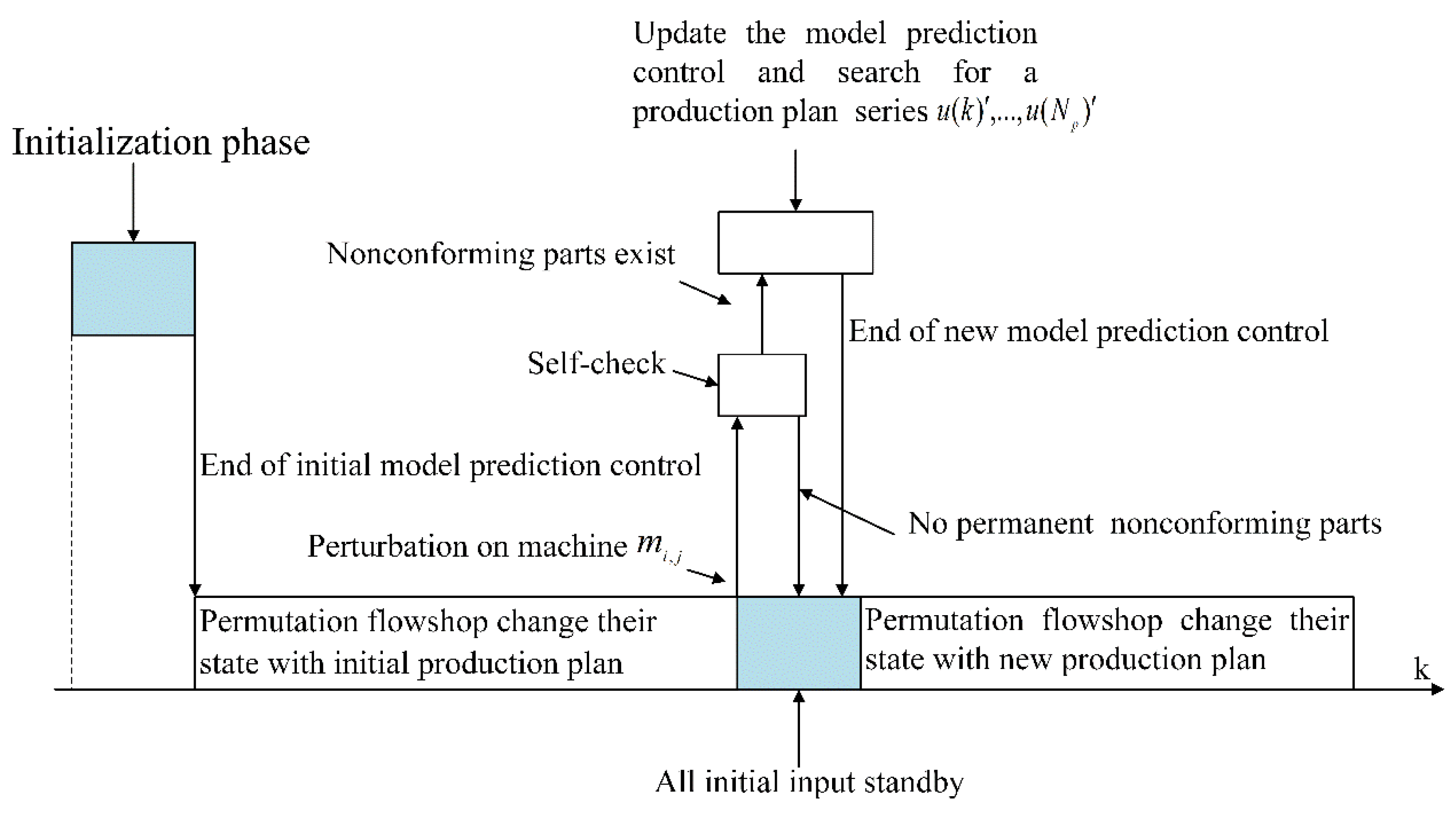
3.2.2. Event-Based Time-Varying Model Predictive Control

Typically, model predictive control only performs the first control sample. After finishing the implementation of the first control sample, the model predictive control will restart with new system information. The job release time is dynamic and uncertain in permutation flowshop; production management will become increasingly difficult. For this reason, an r-WIP optimization approach is presented based on discrete event-driven predictive control. Figure 7 illustrates the implementation architecture of predictive control for the model. In Figure 7, the proposed model predictive control is divided into three steps. Because $A_o(k)$ is a strictly lower triangular matrix with an appropriate number of transitions, a standard state–space model can be obtained by Equations (26) and (27). The $\oplus$ and $\otimes$ mean maximization and addition are, respectively, $a\oplus b=\max (a,b)$ and $a\otimes b=a+b$.

$$X(k)=\overline{A}(k-1)\otimes X(k-1)\oplus \overline{B}(k)\otimes u(k)$$

(26)

$$Y(k)=\overline{C}(k)\otimes X(k),N_{\max }-1\le k\le K$$

(27)

This model predictive control consists of three major steps.

Step 1: A discrete event based on model predictive control driven by current production data and information can be established; it is used to create an initial prediction sequence of production release plan times u (1), u (2), …, u (Np).

Step 2: Through Equations (26) and (27), the state of the replacement flowchart is updated, and real-time data from the physical production system are sensed.

Step 3: If the permutation flowshop has disturbing events, model predictive control can do a self-check to understand how permutation flowshop performance is affected by this random event. If the interference event causes parts to fail, the parameters which the discrete event-driven model predictive control governs are switched, and a new production plan is generated. Otherwise, the production plan needs to be changed every N_p step (if customer demand is deterministic, it is necessary to update the mechanism for releasing the plan every N_p step).

If a disturbing event causes the occurrence of non-conforming parts, set ${\sigma }_j^{\prime }(k_i)={\sigma }_j(k_i)+d_i$. The matrixes $A_o(k^{\prime })$, …, $A_{N_{\max }}(k^{\prime })$, $k^{″}$, and $B(k^{\prime })$ should be updated to $A_o(k^{\prime })$, …, $A_{N_{\max }}(k^{\prime })$, $A(k^{\prime })d$, and $B(k^{\prime })$, $k_i+N_{\max }\ge k^{\prime }\ge k_i$. Then, the space–state equation of a serial production system can be transferred to Equations (28) and (29).

$$X(k^{\prime }+1)=A^{\prime }(k^{\prime })\otimes X(k^{\prime })\oplus B^{\prime }(k+1)\otimes u(k^{\prime }+1)$$

(28)

$$Y(k^{\prime }+1)=C(k^{\prime }+1)\otimes X(k^{\prime }+1),k^{\prime }\ge k_i$$

(29)

In addition, when a disruptive event is perceived, $k^{″}$ components are released into the manufacturing system. (argmax $u(k^{″}):=\left\{k^{″}\left|x_j(k_i)-u(k^{″})>0\right.\right\}$. Then, the new model predictive control can renovate the series of job release times from $k^{″}$ to $k^{″}$ + N_p [35].

4. Solution of the Established Model

If a machine is starved $(S{T}_{i,j}(t))$ at the unit moment t, this indicates that the machine is in a non-fault condition at that moment. But the immediate occupancy rate of the upstream buffer is 0, and the machine has no component input and cannot operate normally. Therefore, the probability of $m_{i,j}$ being in the state $S{T}_{i,j}$ at this moment is shown in Equation (30).

$$P[\Phi (m_{i,j},S{T}_{i,j},t)]=\left\{\begin{array}{l}0,\hspace{1em}\hspace{1em}\hspace{1em}\hspace{1em}\hspace{1em}\hspace{1em}\hspace{1em}\hspace{1em}\hspace{1em}\hspace{1em}\hspace{1em}\hspace{1em}\hspace{1em}\hspace{1em}\hspace{1em}\hspace{1em}\hspace{1em}\hspace{1em}\hspace{1em} i=1\\ P_{i,j}·(P[\Phi (b_{1,1},0,t-1)])·(1-P[\Phi (b_{1,2},0,t-1)]),\hspace{1em}i=2\\ P_{i,j}·P[\Phi (b_{i,j},0,t-1)],\hspace{1em}\hspace{1em}\hspace{1em}\hspace{1em}\hspace{1em}\hspace{1em}\hspace{1em}\hspace{1em}\hspace{1em}\hspace{1em}\hspace{1em} i\ge 3\end{array}\right.$$

(30)

If a machine is blocked $(B{L}_{i,j}(t))$ at the unit moment t, although the machine is in a non-fault state, the downstream buffer has reached its maximum capacity at this moment, the next machine cannot receive parts, and the upstream buffer cannot reduce the inventory. As a result, the machine is blocked because parts cannot be removed after processing. Therefore, the probability of $m_{i,j}$ being in the state $B{L}_{i,j}$ at this moment is shown in Equation (31).

$$P[\Phi (m_{i,j},B{L}_{i,j},t)]=\left\{\begin{array}{l}0,\hspace{1em}\hspace{1em}\hspace{1em}\hspace{1em}\hspace{1em}\hspace{1em}\hspace{1em}\hspace{1em}\hspace{1em}\hspace{1em}\hspace{1em}\hspace{1em}\hspace{1em}\hspace{1em}\hspace{1em}\hspace{1em}\hspace{1em}\hspace{1em}\hspace{1em}\hspace{1em}\hspace{1em}\hspace{1em}i=n,j=3;\\ P_{i,j}·P[\Phi (b_{i,j},Q_{i,j},t-1)]·(P[\Phi (b_{n-1,2},0,t-1]\\ +(1-P[\Phi (b_{{}_{n-1,2}},0,t-1)])·((P_{n+1,3}-P[\Phi (m_{n+1,3},B{L}_{i,j},t]))),\hspace{1em}i=n,j=1;\\ P_{i,j}·P[\Phi (b_{i,j},Q_{i,j},t-1)]·(P[\Phi (b_{n-1,1},0,t-1]\\ +(1-P[\Phi (b_{n-1,1},0,t-1])·((P_{n+1,3}-P[\Phi (m_{n+1,3},B{L}_{i,j},t]))),\hspace{1em}i=n,j=2;\\ P_{i,j}·P[\Phi (b_{i,j},Q_{i,j},t-1)]·(P_{i+1,j}-P[\Phi (m_{i+1,j},B{L}_{i,j},t])),\hspace{1em}\hspace{1em}\hspace{1em} Other.\end{array}\right.$$

(31)

Based on the machine state relationship revealed in Figure 3, the transient productivity of $m_{i,j}$ at time t can be obtained by Equation (32). Figure 3 shows the machine state relationship, and Equation (32) can obtain the instantaneous productivity at time t.

$$\begin{array}{cc}\hfill \mathrm{P}[\Phi {(m}_{i,j}{,\mathrm{PR}}_{i,j},t\left)\right]& =\mathrm{P}[\Phi {(m}_{i,j}{,\mathrm{UP}}_{i,j},t\left)\right]\cap \mathrm{P}[\Phi {(m}_{i,j}{,\mathrm{NST}}_{i,j},t\left)\right]\cap \mathrm{P}[\Phi {(m}_{i,j},{\mathrm{NBL}}_{i,j},t\left)\right]\hfill \\ & ={\mathrm{P}}_{i,j}-P[\Phi (m_{i,j},S{T}_{i,j},t)]-P[\Phi (m_{i,j},B{L}_{i,j},t)]\hfill \end{array}$$

(32)

The change in buffer occupancy rate of the system can be used to describe the transient changes in the permutation flowchart with re-entry links, and the transfer matrix of buffer occupancy can be used to represent the mapping relationship between the system’s pre- and post-transients. Based on the above analysis, Equation (23) to Equation (25) and Equation (30) to Equation (32) are substituted into Equation (9); from this, it can be concluded that the transient state of the permutation flowshop with re-entrant links at the time t and t − 1 is related, so the result is identical to Equation (9). Therefore, if the buffer immediate occupation of the system at time t = 0 and the parameter setting of the machine are given, the buffer level at time t = 1 can be calculated by Equation (9). If this step is repeated, the instantaneous state of the arrangement flowchart with re-entry links can be determined by recursion at any later time. In addition, the process of continuous calculation of buffer occupancy by the recursive method simulates the real running process of permutation flowshop by system modeling. After obtaining the transient information of the system at any time, the transient productivity of a permutation flowshop which has re-entrant links can be calculated by using Equation (32).

5. Case Study

In order to prove the effectiveness of the transient model of the replacement process with re-entry and the feasibility of the analysis method, numerical case studies are performed. In the permutation flowshop environment, as shown in Figure 2, by setting the values of n and r on each production line, seven production systems with different permutation flowshop layouts are selected for example verification; the specific production parameters are shown in

Table 3. Permutation flowshop production parameters.

Layout Code	Machines on the Main Production Line		Rework Line Machine		Machine Separation
	Pi	C	Pi	C	h
1	{0.9, 0.8, 0.8, 0.7}	8	{0.9, 0.8}	4	1
2	{0.9, 0.7, 0.85, 0.8, 0.9}	10	{0.9, 0.8}	4	1
3	{0.9, 0.7, 0.85, 0.8, 0.9}	10	{0.9}	2	1
4	{0.9, 0.7, 0.85, 0.8, 0.9}	10	{0.9, 0.8}	4	1
5	{0.9, 0.7, 0.85, 0.8, 0.9}	10	{0.9, 0.8, 0.7}	6	1
6	{0.9, 0.7, 0.85, 0.8, 0.9, 0.7}	12	{0.9}	2	1
7	{0.9, 0.7, 0.8, 0.8, 0.9, 0.7, 0.8, 0.7, 0.9, 0.9}	20	{0.9, 0.8, 0.9, 0.7, 0.85}	10	1

.

In layout 1, assume that n = 4, r = 1, Line1 and Line2 each have four machines, and there is a test machine on Line3. Also assume that Line1, Line2 and Line3 each have three buffers; Line2 and Line3 each have two machines and two buffers. The reliability model of all machines is set as the Bernoulli model, through Equation (4), to calculate the Line1 production line at any point in $m_{1,1}, m_{2,1}, m_{3,1}, m_{4,1}$ non-fault probability. The maximum storage water in the buffer between machines is set at two processing parts on average. For such a permutation flowshop with a re-entrant link and a total of 13 machines, the first of its parts (the number of the batch of parts $\le Q_{i,j}$) enables all the parts at once to carry on the processing unblocked. In the case of a machine fault which may occur on the main lines, the parts passing through the test machine will be sent to the rework line because there is only one rework machine online; its processing must be less than or equal to one hundred percent success rate. Productivity (PR) is unlikely to be reached one hundred percent. Finally, the maximum productivity PR_max of the system is 0.8959 by simulation. For the last remaining flowchart layout, the average stock level, the productivity (PR), the rework rate (RR), and the power decrease ratio (ECRA) are shown in

Table 4. Results of performance indicators for different permutation flowshop layouts.

Layout Code	Average Inventory Level (${\mathit{Q}}_{\mathit{i},\mathit{j}}$)	Production Rate (PR)	Rework Rate (RR)	Energy-Consuming Reduction Rate (ECRA)
1	0.53	0.8959	0.31	0.11
2	0.47	0.7853	0.26	0.12
3	0.43	0.6792	0.22	0.14
4	0.38	0.5878	0.18	0.18
5	0.34	0.6862	0.26	0.23
6	0.27	0.4865	0.12	0.27
7	0.23	0.4842	0.09	0.31

.

As shown in Table 3 and Table 4, the buffer capacity threshold is kept as 2, and the number of machines and buffers in the permutation flowshop is set, respectively, when the whole production line is a basic flowchart, that is, Layout 1. The number of machines and buffers on the primary production line is very small, so the part processing production line may malfunction and enter the rework line or become blocked on the production line, resulting in a higher rework rate (RR) than other workshop layouts. But when the permutation flowshop reaches $Q_{i,j}$ steady state, layout 1 has the highest productivity (PR) and average inventory level A. On the contrary, when the number of machines and buffers on the main production line increases, the number of machines on the rework line is consistent with layout 1; it can be seen that the rework rate (RR) decreases and the productivity (PR) also decreases. As the research object is the permutation flowshop with re-entrant links, a larger scale means a longer production process and more machines, and the success rate of part processing will greatly increase. Products are in the processing state, so there will be few parts remaining in the buffer. Moreover, the increase in the machine causes the overall production line to be longer; the work of online processes experienced by the products will increase and take more time. At the same time, due to the limitation of buffer stock level $Q_{i,j}$, the biggest permutation flowshop productivity (PR) is affected; the permutation relative to the machine is less and permutation flowshop is lower. Therefore, the productivity (PR) is low. For the layout design problem of permutation flowshop with re-entrant links, a near-optimal solution can be found quickly according to the preset production task type, and can be used to reasonably design the production layout scheme to increase productivity and companies’ economic benefits.

Under the premise of the same production task, for layout 7, the maximum buffer inventory level $Q_{i,j}$ and different processing times are compared, where the probability of the machine being in non-fault condition and the processing cycle are given. In the primary production line, there are 20 machines and the rework has 10 machines in the production line of the re-entrant production line simulation experiment; all the machines still satisfy the information entropy theory and cognitive reliability model, but now the biggest inventory level $Q_{i,j}$ buffer is set to 10 and 100. In certain machines, the maximum inventory level buffer is not the same as the $Q_{i,j}$ comparison. When the buffer between the machine inventory level $Q_{i,j}$ is 20 of the largest processing parts, the machine fault rate is β = 0.15. The following is a comparison of the final productivity (PR) of such re-entrant lines for different processing times. The experimental results are shown in

Table 5. The result when the maximum buffer inventory level $Q_{i,j}$ is 10.

Processing Times	Average Inventory (${\mathit{Q}}_{\mathit{i},\mathit{j}}$)	Production Rate (PR)	Rework Rate (RR)	Energy-Consuming Reduction Rate (ECRA)
10	5	0.8863	0.25	0.206
20	8	0.8886	0.20	0.235
50	10	0.8873	0.15	0.259
80	10	0.8896	0.10	0.293
100	10	0.8912	0.10	0.326

. The results of an experiment where the maximum inventory level of buffer between machines $Q_{i,j}$ is 200 processing parts are presented in

Table 6. The result when the maximum buffer inventory level $Q_{i,j}$ is 100.

Processing Times	Average Inventory (${\mathit{Q}}_{\mathit{i},\mathit{j}}$)	Production Rate (PR)	Rework Rate (RR)	Energy-Consuming Reduction Rate (ECRA)
10	20	0.8852	0.15	0.157
20	25	0.8867	0.17	0.209
50	35	0.8886	0.20	0.248
80	40	0.8898	0.25	0.316
100	60	0.8926	0.25	0.324

.

From Table 5 and Table 6, it can be seen that obtaining a different productivity (PR) solution requires the determination of the number of machines and buffers on the primary line, as well as the different processing periods and buffer capacities. According to the experimental results, if buffer inventory levels are $Q_{i,j}$ for the 20 highest results in the production time, stable production status can be achieved on permutation flowshop; when the biggest buffer inventory levels $Q_{i,j}$ increase, the number of average inventory levels have been $Q_{i,j}$ in the system. That is to say, more and more parts are left in the buffer zone, and if processing time increases, the number of these parts will continue to increase. The replacement process will not reach a stable state. The productivity (PR) is stable in both cases, between 0.8 and 0.9.

Combined with Table 3 and Table 4, in the process of production and processing, when the machine parameters and quantity of the permutation flowshop are determined, the method in this paper can calculate the status of a machine in a certain state under different conditions. Then, it can be used to simulate the productivity (PR) of machines in processing products. It can determine which layout to choose by judging the amount of machines on the entire production line. This production line will optimize the layout of the whole flowshop. For example, different flowshop layouts can be selected when the number of processing parts is large or small, and the permutation flowshop can realize the inspection of the working state of the machine. According to the Bernoulli probability method to calculate the probability of machine fault, it is possible to assign different rework production lines for processing, and finally calculate the productivity (PR) of the product. In addition, regarding the impact of buffer maximum inventory level $Q_{i,j}$ on the energy-saving effect, with the increase in processing times, productivity (PR) shows a decreasing trend; the energy reduction rate (ECRA) gradually increases. Finally, productivity (PR) is 89.26%, and the energy reduction rate (ECRA) is 32.4%. Factories can choose different flowshop layouts according to the actual situation. According to the production demand, the optimal parameter combination is selected by calculating the state of the machine. If factories want to maintain the best productivity (PR) of a permutation flowshop, they can choose the parameter combination with a lower inventory level $Q_{i,j}$. To keep the system inventory level $Q_{i,j}$ minimum, factories can choose $Q_{i,j}$ in combination with higher productivity (PR).

When assessing the efficacy of control strategies for permutation flowshop operations, it is important to consider not only the instantaneous state of the process J_in, but also the tracking error J_out of the reference signal. In Figure 8a, the tardiness values for layouts 1 to 7 are Y (700)-r (700) = 4261 s, 4725 s, 5125 s, 5944 s, 4958 s, 8027 s, and 10,669 s, respectively. Layout 1 can also achieve maximum throughput in the presence of non-conforming parts, but this can only be achieved by maintaining a high level of work-in-progress (WIP) buffering. In addition, the flexibility of event model predictive control (WIP) and discrete model predictive control (DMPC) in work-in-progress (WIP) is limited when machines are lacking or blocked. In Figure 8b, the circle represents the delay gap Jout (k + 1) − Jout (k) for different layouts. It can be seen from the results that when additional work is actively added in the unpredictable event, it is possible to increase the throughput of the sorting process by the event model prediction control and the discrete model prediction of the WIP. While DPM has similar output performance as WIP, it is not highly stable, as illustrated in Figure 8a of the drawing. In particular, r-WIP in discrete model predictive control of WIP is highly volatile, as illustrated in Figure 9b, which can add complexity to process management. On the other hand, WIP, an event model predictive control, is able to keep a constant WIP level through real-time adjustment of production schedule. Specifically, the r-WIP is very volatile in discrete model predictive control; as illustrated in Figure 9b, the complexity of process management may increase. On the contrary, if the production plan is adjusted in real time, event model predictive control of work-in-progress can maintain a constant level of it.

In Figure 9, we can observe the r-WIP metrics for seven distinct layouts. At each production step, r-WIP can be computed. Figure 9a illustrates that the r-WIP of the first layout exhibits a consistent linear increase alongside the production plan. Meanwhile, Figure 9b provides a graphical representation of the r-WIP for layouts 2 to 7 in a block diagram format, highlighting the fact that r-WIP values for other layouts remain below that of layout 2.

The average r-WIP for layout 2 hovers at approximately 24 units, while for the other layouts, the corresponding averages stand at 13 units, 6 units, 15 units, 7 units, and 21 units for layouts 3, 4, 5, 6, and 7, respectively. If we allocate preventive work-in-progress within the production system, it can lead to a notable enhancement in the effectiveness of discrete model predictive control and event model predictive control. To further investigate the average r-WIP required for event model predictive control WIP to achieve the same throughput as layout 2, a series of sensitivity experiments pertaining to r-WIP constraints were conducted within the scope of this study.

The results reveal that the event model predictive control WIP can achieve an equivalent throughput to various layouts when the average r-WIP is approximately 14.3 units. This average r-WIP value is smaller than the reference value associated with layout 2. As part of this study, numerous sensitivity experiments were carried out concerning the r-WIP constraint. This allowed the author to gain insights into the requisite average r-WIP for event model predictive control WIP to match the throughput of layout 2. The findings underscore that, with an average r-WIP of 14.3 units, the event model predictive control WIP can achieve parity with various layouts, even when layout 2 surpasses this particular benchmark.

Furthermore, in comparison to discrete model predictive control, both WIP and event model predictive control exhibit reduced flexibility only in cases where the duration of interference events is more prolonged. As depicted by the circular graph in Figure 8b, variations in the delay gap, denoted as Jout (k + 1) − Jout (k), occur under different conditions for discrete model predictive control WIP and event model predictive control WIP, resulting in distinct delay gaps. This signifies that it is only when additional work-in-progress is introduced prior to unforeseen events that discrete model predictive control WIP and event model predictive control WIP can enhance the production system’s throughput.

Although discrete model predictive control WIP demonstrates similar output performance when compared to event model predictive control WIP, as illustrated in the figure, the stability, as shown in Figure 8a, is notably compromised. In discrete model predictive control, work-in-progress fluctuations are pronounced, as is evident in Figure 9b, potentially escalating the challenges associated with process management. Conversely, by adjusting the production release plan in real time, event model predictive control WIP can maintain a consistent level of work-in-progress, thereby ensuring a more stable operational environment.

To further verify the effectiveness of the proposed method in practical cases, a simulation was carried out for the production process of flowshop layout 7, and the reliability (R) of the machine was the same, varying evenly from 0.6 to 1 at 0.1 intervals. All buffers have the same maximum inventory level $Q_{i,j}$, which increases evenly from 0 to 100. For all parameter settings, the productivity (PR) obtained by the method in this paper, the classical steady-state method [36], and the traditional method are shown in Figure 10 and Figure 11.

Under the same production line, permutation flowshop layout, and production tasks, the method in this paper is used to process parts in batches. Figure 10 shows that the method and classical steady-state method productivity (PR) will be considered as the change of reliability (R) and the maximum inventory level $Q_{i,j}$; the method of productivity (PR) will increase with an increase in the reliability (R), resulting in an increase in productivity (PR) calculation error. However, compared with the conventional steady-state method, the error of (PR) calculation is lower. The results obtained by the classical steady-state method [36] are at the low point, which proves the feasibility of the proposed method.

It is clear from Figure 11 that the same production tasks in the permutation flowshop layout, the reliability (R), and largest inventory levels under the premise of the same. The present method and the traditional method of productivity (PR) will go along with the reliability ® increases, but based on the method of productivity, (PR) is higher than the traditional method of productivity (PR) and the maximum inventory level $Q_{i,j}$ = 100. The difference between the two can be as much as 5%. Therefore, under the premise of the same layout and same productivity (PR), the maximum inventory level required in this paper $Q_{i,j}$ is small. In the case of the same layout and the same maximum inventory level $Q_{i,j}$, the productivity (PR) of the proposed method is high.

6. Conclusions and Future Work

This paper conducts an in-depth analysis of the interplay of flexibility and uniqueness in the substitution process within the framework of Bernoulli’s theory. To begin, it commences by assessing the reliability of the production process and the operational states of the machinery and buffers. Subsequently, it employs state transition probability functions to model potential blockages or resource shortages, deriving the transient mapping relationship matrix of the system.

Furthermore, this research establishes a transient productivity model tailored for permutation flowshops and gauges the essential production performance indicators through a recursive methodology. Notably, it also formulates an instantaneous productivity model for the permutation process, employing recursive techniques to evaluate the key production metrics.

To address the challenges of intelligent control in permutation flowshops and to furnish comprehensive, real-time production insights, a model predictive control system based on discrete event-driven feedback is employed. As a result of these research outcomes, there is a discernible enhancement in the ability to perceive and predict work-in-progress, leading to significant savings in human resources.

The presence of re-entrant links within this permutation flowshop production system ensures that the entire production line remains uninterrupted even in the event of machinery faults, thereby augmenting the production efficiency in part processing. The proposed model has optimized the layout of the arrangement process and enables the prediction and analysis of potential congestion or resource shortages. This offers an invaluable theoretical underpinning for making intelligent decisions in the realm of complex part production.

In future research endeavors, we will place a strong emphasis on several key aspects. Firstly, we intend to utilize this algorithm to schedule and manage diverse production lines, broadening its applicability and effectiveness across various industrial contexts. Secondly, we will delve into the exploration of alternative approximation algorithms, such as local search and simulated annealing, to address the problem at hand. This expansion of algorithmic theory will enrich our problem-solving toolkit and provide more robust solutions. Thirdly, our objective is to enhance the proposed model, enabling a comprehensive analysis and optimization of the real-time state of the products. This advancement will allow for proactive planning and decision making. Lastly, we will direct our research efforts towards dynamic production decision equations, leveraging the power of deep reinforcement learning. This approach promises to deliver more adaptive and data-driven production decisions, ensuring greater efficiency and responsiveness in dynamic manufacturing environments.

References

1. Gheisariha, E.; Tavana, M.; Jolai, F.; Rabiee, M. A simulation–optimization model for solving flexible flow shop scheduling problems with rework and transportation. Math. Comput. Simul. 2021, 180, 152–177. [Google Scholar] [CrossRef]
2. Subramaniyan, M.; Skoogh, A.; Salomonsson, H.; Bangalore, P.; Bokrantz, J. A data-driven algorithm to predict throughput bottlenecks in a production system based on active periods of the machines. Comput. Ind. Eng. 2018, 125, 533–544. [Google Scholar] [CrossRef]
3. Tao, F.; Zhang, M.; Cheng, J.; Qi, Q. Digital twin workshop: A new paradigm for future workshop. Comput. Integr. Manuf. Syst. 2017, 23, 1–9. [Google Scholar]
4. Chen, J.; Jia, Z.; Huang, L. Multi-type products and dedicated buffers-based flexible production process analysis of serial Bernoulli lines. Comput. Ind. Eng. 2021, 154, 107167. [Google Scholar] [CrossRef]
5. Yan, C.B.; Cheng, X.; Gao, F.; Guan, X. Formulation and solution methodology for reducing energy consumption in two-machine Bernoulli serial lines. IEEE Trans. Autom. Sci. Eng. 2020, 19, 522–530. [Google Scholar] [CrossRef]
6. Pei, Z.; Yang, P.; Wang, Y.; Yan, C.-B. Energy consumption control in the two-machine Bernoulli serial production line with setup and idleness. Int. J. Prod. Res. 2023, 61, 2917–2936. [Google Scholar] [CrossRef]
7. Wang, X.; Dai, Y.; Jia, Z. Energy-efficient on/off control in serial production lines with Bernoulli machines. Flex. Serv. Manuf. J. 2022, 1–26. [Google Scholar] [CrossRef]
8. Yan, C.B.; Zheng, Z. Problem formulation and solution methodology for energy consumption optimization in Bernoulli serial lines. IEEE Trans. Autom. Sci. Eng. 2020, 18, 776–790. [Google Scholar] [CrossRef]
9. Hadžić, N.; Ložar, V.; Opetuk, T.; Andrić, J. A finite state method in improvement and design of lean Bernoulli serial production lines. Comput. Ind. Eng. 2021, 159, 107449. [Google Scholar] [CrossRef]
10. Hadžić, N.; Ložar, V.; Opetuk, T.; Kunkera, Z. The Bernoulli Assembly Line: The Analytical and Semi-Analytical Evaluation of Steady-State Performance. Appl. Sci. 2022, 12, 12447. [Google Scholar] [CrossRef]
11. Liu, M.; Xie, J.; Wu, H.; Fu, J.; Ding, G. Research on Workshop Logic Modeling and Simulation Based on Finite State Machine. J. Syst. Simul. 2023, 35, 853–861. [Google Scholar]
12. Öztop, H.; Tasgetiren, M.F.; Kandiller, L.; Eliiyi, D.T.; Gao, L. Ensemble of metaheuristics for energy-efficient hybrid flowshops: Makespan versus total energy consumption. Swarm Evol. Comput. 2020, 54, 100660. [Google Scholar] [CrossRef]
13. Tang, D.; Wang, J.; Ding, X. Order-Driven Dynamic Resource Configuration Based on a Metamodel for an Unbalanced Assembly Line. Machines 2022, 10, 508. [Google Scholar] [CrossRef]
14. Zhao, R.; Zou, G.; Su, Q.; Zou, S.; Deng, W.; Yu, A.; Zhang, H. Digital Twins-Based Production Line Design and Simulation Optimization of Large-Scale Mobile Phone Assembly Workshop. Machines 2022, 10, 367. [Google Scholar] [CrossRef]
15. Chen, J.; Shen, Z.J.M. Fast Approximations for Dynamic Behavior in Manufacturing Systems with Regular Orders: An Aggregation Method. IEEE Robot. Autom. Lett. 2023, 8, 7122–7129. [Google Scholar] [CrossRef]
16. Pagone, E.; Haddad, Y.; Barsotti, L.; Dini, G.; Salonitis, K. A stochastic evaluation framework to improve the robustness of manufacturing systems. Int. J. Comput. Integr. Manuf. 2023, 36, 966–984. [Google Scholar] [CrossRef]
17. Mo, F.; Rehman, H.U.; Monetti, F.M.; Chaplin, J.C.; Sanderson, D.; Popov, A.; Maffei, A.; Ratchev, S. A framework for manufacturing system reconfiguration and optimisation utilising digital twins and modular artificial intelligence. Robot. Comput. Integr. Manuf. 2023, 82, 102524. [Google Scholar] [CrossRef]
18. Wang, X.; Gu, W.; Liu, S.; Guo, Z.; Zhan, Y. Modeling of Bernoulli production line with rework loop for real-time work-in-process optimization in permutation flowshop. In Proceedings of the IEEE 6th Advanced Information Technology, Electronic and Automation Control Conference, Beijing, China, 3–5 October 2022; pp. 1266–1270. [Google Scholar]
19. Wang, X.; Dai, Y.; Wang, L.; Jia, Z. Transient Analysis and Scheduling of Bernoulli Serial Lines with Multi-Type Products and Finite Buffers. IEEE Trans. Autom. Sci. Eng. 2022, 20, 2367–2382. [Google Scholar] [CrossRef]
20. Ma, C.; Jia, Z.; Wang, X.; Ni, Z. Transient Performance Evaluation with Finite Production Run-based Serial Lines: Bernoulli Quality Model. In Proceedings of the 2021 International Conference on Cyber-Physical Social Intelligence (ICCSI), Beijing, China, 18–20 December 2021; pp. 1–6. [Google Scholar]
21. Bachar, R.K.; Bhuniya, S.; Ghosh, S.K.; AlArjani, A.; Attia, E.; Uddin, S.; Sarkar, B. Product outsourcing policy for a sustainable flexible manufacturing system with reworking and green investment. Math. Biosci. Eng. 2023, 20, 1376–1401. [Google Scholar] [CrossRef]
22. Zhou, B.; Zha, W. Performance evaluation and optimization model for closed-loop production lines considering preventive maintenance and rework process. Proc. Inst. Mech. Eng. Part E J. Process Mech. Eng. 2023, 09544089231160514. [Google Scholar] [CrossRef]
23. Sun, H.; Xia, T.; Shi, Y.; Leng, B.; Wang, H. Online energy consumption optimization of rework production system based on digital twin. Comput. Integr. Manuf. Syst. 2023, 29, 11. [Google Scholar]
24. Jia, Z.; Ni, Z.; Ma, C. Dynamic Process Modeling and Real-Time Performance Evaluation of Rework Production System with Small-Lot Order. IEEE Robot. Autom. Lett. 2023, 8, 2874–2881. [Google Scholar] [CrossRef]
25. Khezri, A.; Homri, L.; Etienne, A.; Dantan, J.-Y.; Lanza, G. A Framework for integration of resource allocation and reworking concept into design optimisation problem. IFAC Pap. 2022, 55, 1037–1042. [Google Scholar] [CrossRef]
26. Chen, J.; Mohammed, A.; Alexopoulos, T.; Setchi, R. Collaborative human-robot assembly: Methodology, simulation and industrial validation. In International Conference on Sustainable Design and Manufacturing; Springer: Singapore, 2022; pp. 181–190. [Google Scholar]
27. Lago Alvarez, A.; Mohammed, W.M.; Vu, T.; Ahmadi, S.; Martinez Lastra, J.L. Enhancing Digital Twins of Semi-Automatic Production Lines by Digitizing Operator Skills. Appl. Sci. 2023, 13, 1637. [Google Scholar] [CrossRef]
28. Shi, J.; Chen, M.; Ma, Y.; Qiao, F. A new boredom-aware dual-resource constrained flexible job shop scheduling problem using a two-stage multi-objective particle swarm optimization algorithm. Inf. Sci. 2023, 643, 119141. [Google Scholar] [CrossRef]
29. Li, Y.; Chang, Q.; Ni, J.; Brundage, M.P. Event-based supervisory control for energy efficient manufacturing systems. IEEE Trans. Autom. Sci. Eng. 2018, 15, 92–103. [Google Scholar] [CrossRef]
30. Zhou, B.; Su, Y. Energy-saving analysis of serial production lines based on the changeable buffers’ storage. J. Harbin Eng. Univ. 2016, 37, 832–836. [Google Scholar]
31. Xin, W.; Zequn, Z.; Dunbing, T. Energy-saving Oriented Multi-objective Shop Floor Scheduling for Mixed-line Production of Missile Components. J. Mech. Eng. 2018, 54, 45–54. [Google Scholar]
32. Zhang, H.; Tang, D. Output Prediction and Disturbance Analysis of Manufacturing Networks Based on State Space. J. Mech. Eng. 2016, 52, 166–174. [Google Scholar] [CrossRef]
33. Pan, Q.K.; Wang, L.; Li, J.Q.; Duan, J.H. A novel discrete artificial bee colony algorithm for the hybrid flowshop scheduling problem with makespan minimization. Omega 4 2014, 5, 42–56. [Google Scholar] [CrossRef]
34. Cao, Y.; Subramaniam, V.; Chen, R. Performance evaluation and enhancement of multistage manufacturing systems with rework loops. Comput. Ind. Eng. 2011, 62, 161–176. [Google Scholar] [CrossRef]
35. Chen, W.; Liu, H.; Qi, E. Discrete Event-driven Model Predictive Control for Real-time Work-in-process Optimization in Serial Production Systems. J. Manuf. Syst. 2020, 55, 132–142. [Google Scholar] [CrossRef]
36. Komenda, J.; Lahaye, S.; Boimond, J.-L.; Boom, T.V.D. Max-plus algebra in the history of discrete event systems. Annu. Rev. Control 2018, 45, 240–249. [Google Scholar] [CrossRef]
Figure 1. Traditional serial production line.
Machines 12 00020 g001
Figure 2. A Replacement Process Model with Re-entry Links.
Machines 12 00020 g002
Figure 3. Machine state diagram.
Machines 12 00020 g003
Figure 4. Three machine instantaneous state transition relationships.
Machines 12 00020 g004
Figure 5. The instantaneous transfer relation of buffer b i , j at time t.
Machines 12 00020 g005
Figure 6. The logic of the model predictive control.
Machines 12 00020 g006
Figure 7. Model Predictive Control Based on Discrete Events’ Implementation Structure.
Machines 12 00020 g007
Figure 8. Permutation flowshop throughput with various control mechanisms. (a) Y(700)-r(700), (b) J1 (k + 1)-J1 (k).
Machines 12 00020 g008
Figure 9. r-WIP with different control mechanisms. (a) The WIP in layout 1, (b) The WIP in layout 2-layout 7.
Machines 12 00020 g009
Figure 10. The calculation results of the proposed method and the classical steady-state performance algorithm under different parameter settings.
Machines 12 00020 g010
Figure 11. Comparison of calculation results between the proposed method and the traditional method under different parameter settings.
Machines 12 00020 g011