Article

A Novel Load Extrapolation Method for Multiple Non-Stationary Loads on the Drill Pipe of a Rotary Rig

1
Xuzhou Xugong Foundation Construction Machinery Co., Ltd., Xuzhou 221018, China
2
School of Mechanical and Aerospace Engineering, Jilin University, Changchun 130025, China
*
Author to whom correspondence should be addressed.
Machines 2024, 12(1), 75; https://doi.org/10.3390/machines12010075
Submission received: 1 December 2023 / Revised: 3 January 2024 / Accepted: 16 January 2024 / Published: 19 January 2024
(This article belongs to the Section Machine Design and Theory)

Abstract

:
The drill pipe of a rotary rig is subject to the dynamic influence of non-stationary loads, including rotation torque and applied force. In order to address the challenge of simultaneously extrapolating multiple non-stationary loads, a novel extrapolation framework is proposed. This framework utilizes rainflow counting to obtain mean and amplitude sequences of the loads. The extreme values of the amplitude sequence are fitted using the Generalized Pareto Distribution (GPD), while the median values are fitted using the Double Kernel Density Estimation (DKDE). By extrapolating the Inverse Cumulative Distribution Function (ICDF) based on the fitted distribution, a new amplitude sequence can be derived. The combination of this extrapolated amplitude sequence with the original mean sequence forms a new load spectrum. The results of applying the proposed extrapolation method to the drill pipe of a rotary rig demonstrate the ability of the method to yield conservative extrapolation results and accurately capture the variations in damage under the original working conditions.

1. Introduction

The rotary drilling rig is a type of large-scale engineering equipment that is extensively utilized in highway and bridge engineering, water conservancy engineering, and urban construction [1]. The drill pipe is a critical component of the rotary drilling rig, and there has been significant attention given to the compilation of its load spectrum and the calculation of its fatigue life. The load spectrum can be employed to evaluate the structural life, analyze bench tests, and consequently optimize the main structure to enhance durability [2,3]. In general, testing large equipment poses challenges due to its difficulty and high cost. A rational load spectrum extrapolation method is crucial to accurately reflect the load variations throughout the entire life cycle of the structure.
As shown in Figure 1a, the drill pipe is subject to both rotation torque and applied force. The torque and force, obtained from the stress solution, are illustrated in Figure 1b. None of the existing methods are suitable for the compilation and extrapolation of the drill pipe load spectrum. The compiled and extrapolated load spectrum should take into account the simultaneous variations in both torque and force. The extrapolation based on the rainflow matrix method does not meet the aforementioned requirements, while the time-domain extrapolation approach is constrained by the stationary properties of the loads, making it unsuitable for non-stationary load scenarios. Therefore, there is an urgent demand for load extrapolation methods for multiple non-stationary loads acting simultaneously.

1.1. Related Works

1.1.1. Approach for Keeping the Load Sequence

Multiple load sequences can be statistically counted in two ways: online and offline, depending on whether the order of actions is preserved.
Online counting ensures the load sequence order, taking into account the effects of temperature gradients [4] and time-dependent damage mechanisms [5,6], but it may be limited by data storage and computational resources [7]. Moreover, online real-time counting may neglect the residual large loads, which can cause significant damage.
The purpose of offline counting methods is to retain the load sequence without requiring real-time processing [8]. For example, the top-level-up counting technique considers the load sequence, but it only records the changes in load magnitude [9]. Additionally, there is an iterative RFC algorithm that preserves the cycle order, but it has high complexity and a long computation time [10]. However, the methods for actively retaining the non-stress loads are still imperfect. The integration of extrapolation knowledge with the load sequence is an undeveloped area.

1.1.2. Load Extrapolation

Currently, load spectrum extrapolation methods can be primarily categorized into three main approaches: parametric extrapolation, nonparametric extrapolation, and time-domain extrapolation [11,12]. Both parametric and nonparametric methods rely on statistical rainflow matrices [13]. In the parametric method, amplitude and mean distributions are parametrically fitted, and extrapolation is performed based on the estimated number of potential load cycles. On the other hand, the nonparametric method utilizes kernel density to estimate potential distribution and extrapolate the load accordingly [2]. The prototypical time-domain extrapolation method, proposed by P. Johannesson, is based on the peak over threshold (POT) Pareto parameter model [14].

1.1.3. Advanced Load Extrapolation Method

Advanced load spectrum extrapolation methods emphasize the integration of load extrapolation with sophisticated preprocessing techniques and simulation-based or data-driven approaches for load extrapolation. Zhang et al. [15] determined the optimal threshold for extreme value extrapolation based on gray correlation. Shangguan et al. [16] used the wavelet transform to process the measured loads, preserving most of the damage while making it possible to reduce the length of the time series. In terms of simulation-based or data-driven approaches, Poloni et al. [17] used Gaussian process strain extrapolation to reconstruct displacements on beam or shell structures. Wen et al. [18] recognized the high-work-intensity segment of a tractor load spectrum using a modified LSTM network. Other approaches include the use of machine learning [19,20] and deep learning [21,22] for load prediction and estimation, which can lead directly to the relevant load spectrum.

1.2. Motivation and Contribution

We propose a novel load extrapolation framework to effectively address the scenario of multiple non-stationary loads acting simultaneously. The torque and force loads are first processed using rainflow counting to obtain a sequence of amplitude and mean values. These values are then arranged in the order of their occurrence. To capture extreme amplitudes, the POT method is utilized in the proposed framework. By fitting the extreme loads using a Generalized Pareto Distribution (GPD), the extrapolation of extreme loads can be performed effectively. The median amplitudes are fitted using a Diffusion Kernel Density Estimation (DKDE) [23,24] method. This allows for an accurate estimation of the underlying probability density function, which is then used to extrapolate the median amplitudes accordingly. The final load spectrum is obtained by combining the mean sequence and the extrapolated amplitude sequence. The main contributions of the proposed load spectrum extrapolation framework are as follows:
  • Consideration of multiple non-stationary loads. The framework addresses the challenge of multiple non-stationary loads acting simultaneously, allowing for a more realistic representation of load variations.
  • Integration of rainflow counting and POT method. By incorporating rainflow counting and the POT method, the framework effectively captures extreme load amplitudes and enables accurate extrapolation of the load spectrum.
  • DKDE method for median amplitudes estimation. The DKDE method is employed to fit and extrapolate median amplitudes, providing a reliable estimation of load behavior.
  • Comprehensive load spectrum representation. A load spectrum that accounts for both median and extreme load variations, offering a more complete understanding of the load profiles for structural analysis.

2. Methods

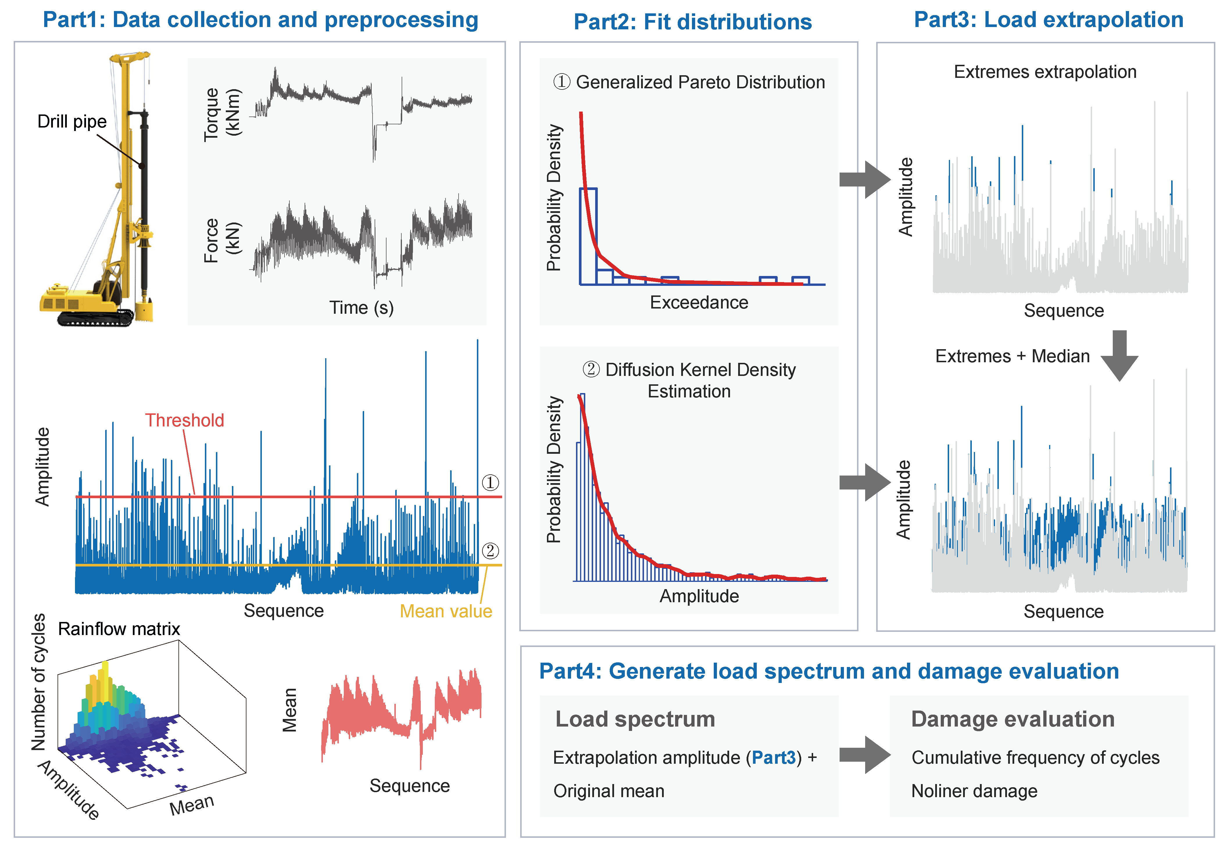
2.1. Proposed Load Spectrum Extrapolation Framework

The specific steps involved in the multiple non-stationary load extrapolation framework shown in Figure 2 are as follows:
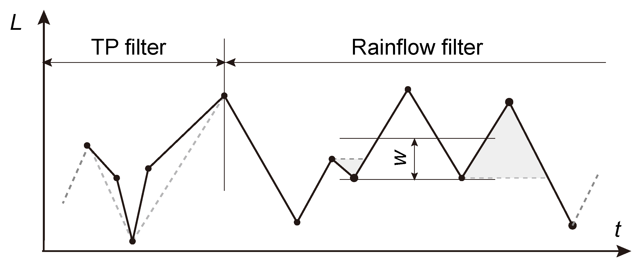
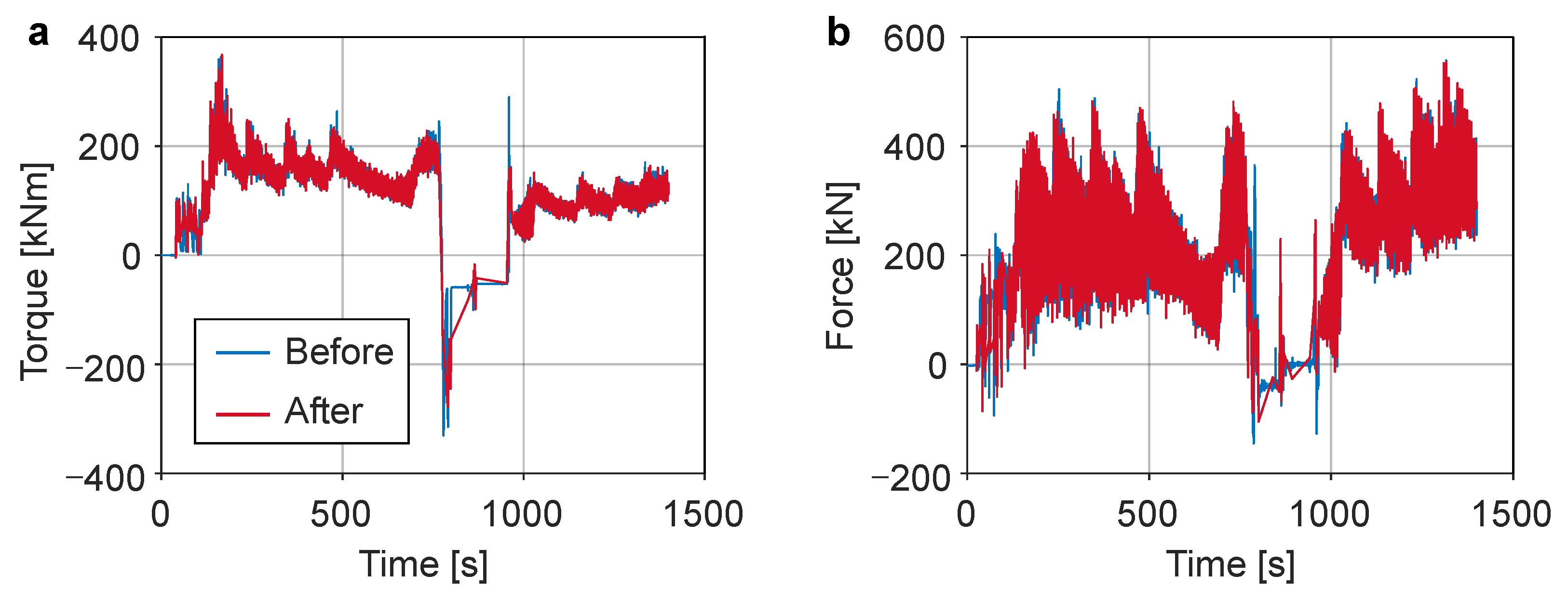
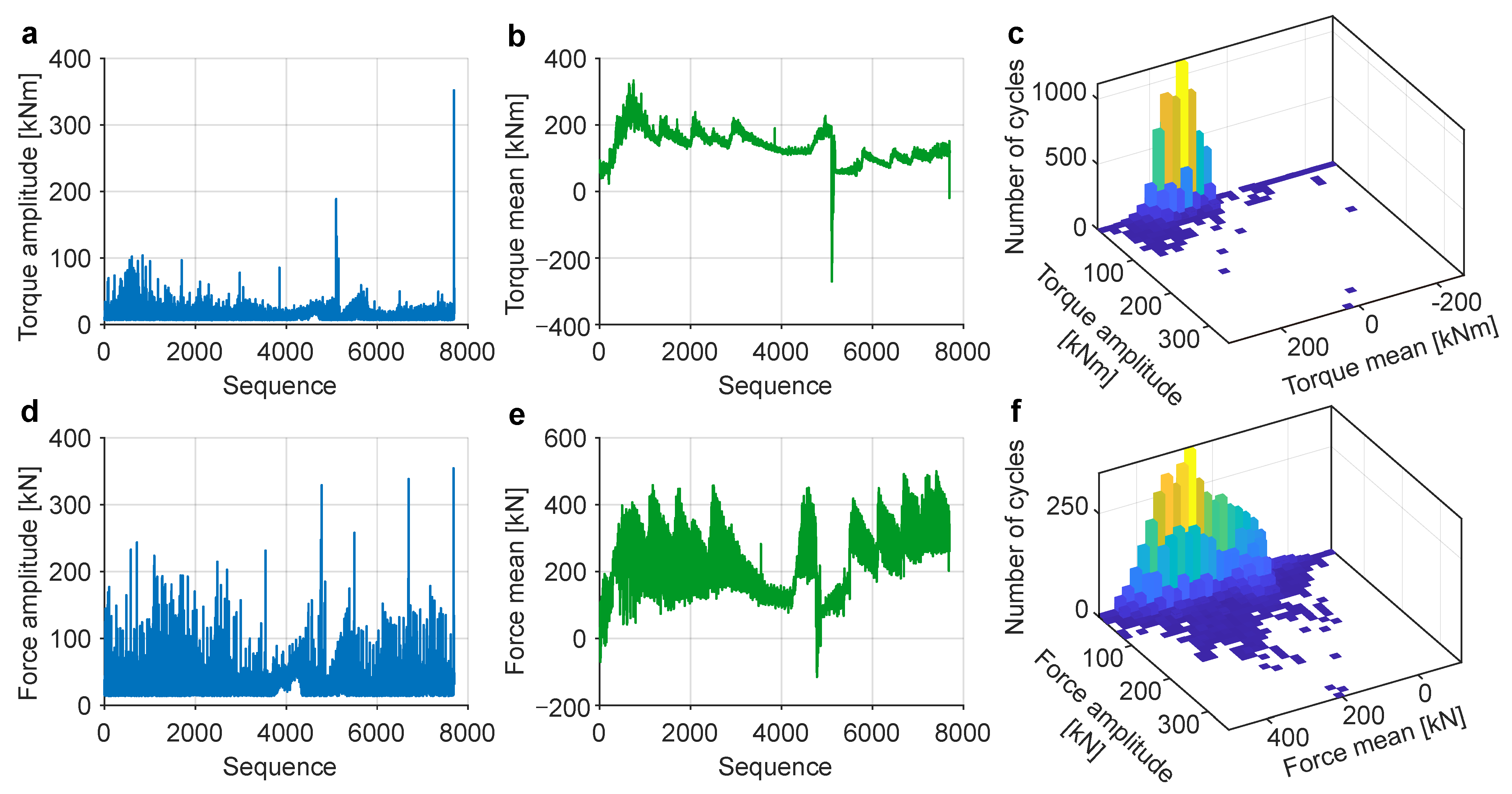
  • Data collection and preprocessing. The stress data of the drill pipe are converted into torque and force data, which are filtered and synchronized with rainflow counting to obtain the same mean and amplitude sequences.
  • Fit distributions. The amplitude sequence is analyzed by fitting distributions to different parts of the data. Specifically, a GPD fit is applied to the portion beyond a specified threshold, while a DKDE fit is used for the section between the median and the threshold. This fitting process allows for capturing the characteristics and modeling the distribution of amplitudes within different ranges of the data.
  • Load extrapolation. To extrapolate the amplitude in the order of occurrence, an inverse cumulative distribution function (ICDF) is established based on the probability density function (PDF) of the distribution function. Using the established ICDF, we can extrapolate the amplitudes in the order of occurrence by generating random numbers from a uniform distribution and mapping them to corresponding amplitude values using the ICDF.
  • Generate load spectrum and damage evaluation. The extrapolated amplitude sequence, obtained using the inverse cumulative distribution function, is combined with the original mean sequence to form a load spectrum, and nonlinear damage is used to assess the damage of the current extrapolated load spectrum.

2.2. Data Preprocessing

Before obtaining the mean and amplitude of the rainflow count for torque and force, the loads undergo a filtering process that consists of two steps: a turning point filter and a hysteresis filter based on the rainflow counts, as shown in Figure 3 [25].
Turning Point Filter. The turning points of the load data L ( t ) are identified. Turning points represent the transition from one load direction to another.
T P ( L ( t ) ) = { L ( t 1 0 ) , L ( t 2 0 ) , , L ( t N 0 ) }
where t 1 0 , , t N 0 are the time points of the local extremes. By filtering out insignificant turning points, such as those caused by noise or measurement errors, the data are refined to include only significant turning points.
Hysteresis Filter. Based on the rainflow counts, a hysteresis filter is applied to remove minor load cycles that do not significantly contribute to fatigue damage. This removes all turning points that correspond to rainflow cycles with the ranges below the given threshold w, resulting in
T P ( L ( t ) , w ) = { L ( t 1 ) , L ( t 2 ) , , L ( t N ) }
where t 1 , , t N are the time points of the local extremes.
The filter process helps to capture the major load cycles with higher amplitudes and eliminate smaller cycles that may not significantly affect the structural fatigue life.

2.3. Distribution Fitting

The fitting of the distribution in the proposed framework involves two parts: GPD fitting for suprathreshold extremes and DKDE fitting for medium loads.

2.3.1. Generalized Pareto Distribution Model

After counting the rainflow, the amplitude and mean values of the torque and force in the order of occurrence are obtained. Based on the POT method for selecting extreme values above the threshold u, the upper tail is fitted using the GPD. The cumulative distribution function (CDF) of the GPD is expressed as [26]
G [ u ] ( x ; σ , ξ ) = 1 1 + ξ x u σ 1 ξ , ξ 0 1 exp x u σ , ξ = 0 , x u , 1 + ξ x u σ > 0
By calculating the first derivative of the distribution function (Equation (3)), the probability density function (PDF) of the GPD can be obtained.
g [ u ] ( x ; σ , ξ ) = 1 σ 1 + ξ x u σ 1 + ξ ξ , ξ 0 1 σ exp x u σ , ξ = 0 , x u , 1 + ξ x u σ > 0
where x is the sample value, σ is the scale parameter, and ξ is the shape parameter.

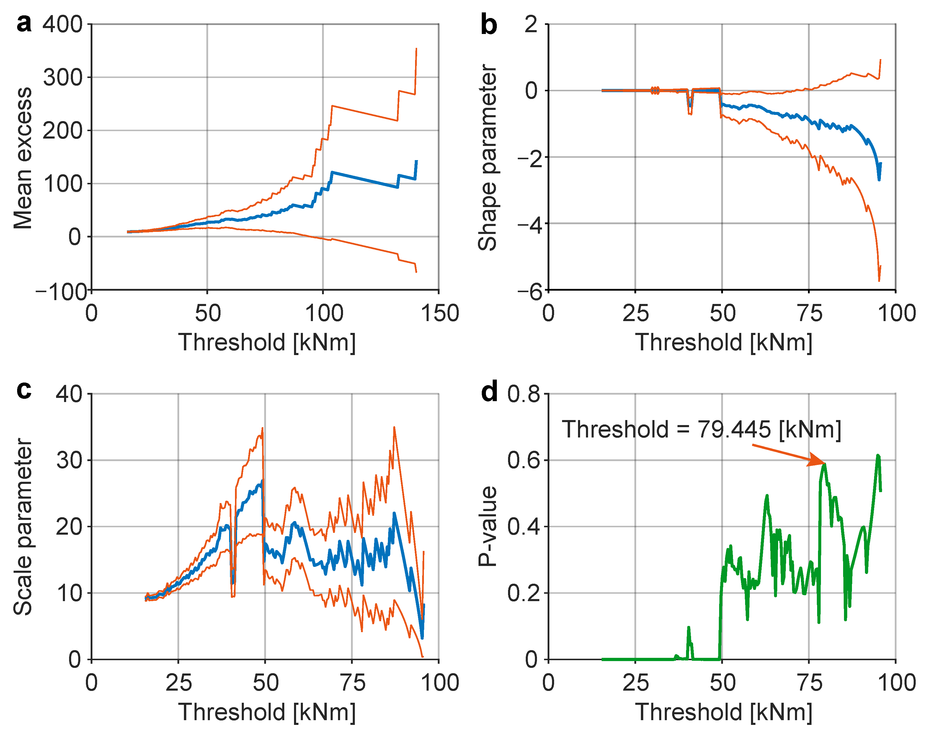
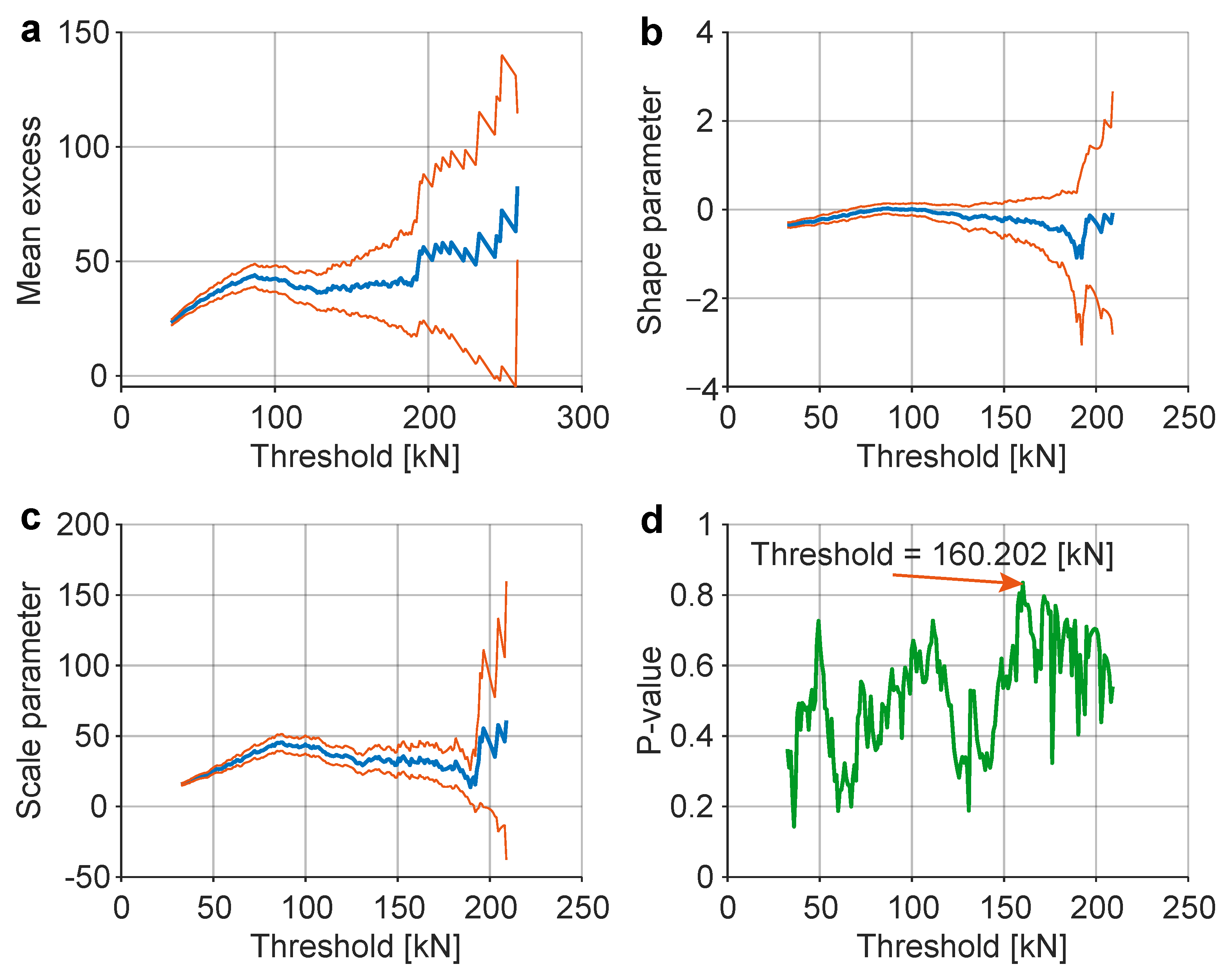
2.3.2. Threshold Selection

In the GPD, one of the main concerns is the determination of appropriate thresholds. The selection of thresholds is crucial as it affects the estimation of the tail behavior and the accuracy of the extrapolation for extreme values. The choice of thresholds should strike a balance between capturing enough extreme events for reliable estimation and avoiding excessive inclusion of non-extreme events that can lead to biased results.
Various statistical methods, such as the mean excess plot, Hill plot, or graphical techniques, can be employed to assist in determining suitable thresholds for GPD estimation based on the specific characteristics of the dataset and the desired level of accuracy.
Mean exceedance is the most commonly used method of threshold selection. The mean excess function (MEF) of the GPD can be obtained as follows
e ( u ) = E ( x u x > u ) = σ 1 ξ + u ξ 1 ξ , ξ < 1
Furthermore, once the threshold is selected, the shape and scale parameters of the GPD can be estimated using the maximum likelihood estimation method. This estimation allows for quantifying the shape of the distribution and its scale relative to the threshold.
To evaluate the goodness of fit, a χ 2 test can be performed to assess the difference between the observed extreme-value distribution and the estimated GPD distribution. The test calculates a p-value, and a p-value close to 1 indicates a good fitting effect, suggesting that the estimated GPD distribution adequately captures the characteristics of the observed extreme values.

2.3.3. Diffusion Kernel Density Estimation

Kernel density estimation (KDE) is an important nonparametric estimation method. Consider a random variable X [ X 1 , , X n ] with a true probability distribution f ( x ) [27]:
f ^ ( x ; h ) = 1 n i = 1 n K x , X i ; h = 1 n h i = 1 n K x X i h
where K ( · ) is a kernel function, and h is a bandwidth. The two most important parameters to be determined in kernel density estimation are the choice of the kernel function and the bandwidth.
The kernel function determines the shape and characteristics of the individual kernels placed at each sample point. Commonly used kernel functions include the Gaussian (or normal) kernel, Epanechnikov kernel, and uniform kernel. The bandwidth parameter controls the width or spread of the kernel function. It determines the extent to which nearby sample points contribute to the density estimate. There are various methods available for selecting the kernel function and bandwidth, such as cross-validation, plug-in methods, and rule-of-thumb approaches.
In the DKDE, when the domain is [ 0 , 1 ] , it is divided into N segments as part of the estimation process. The PDF of the DKDE can be expressed as [23]
f ^ ( x , t ) k = 0 N 1 a k exp k 2 π 2 t 2 cos k π ( 2 j + 1 ) 2 N
where t is the bandwidth of the DKDE, and the coefficient a k is
a k = 1 , k = 0 2 j = 0 N 1 P ( j ) cos ( 2 j + 1 ) k π 2 N , k = 1 , 2 , , N 1
where P ( j ) is the probability that X i happens in the interval [ j / N , ( j + 1 ) / N ] .
Indeed, the DKDE method employs an improved plug-in methodology that is fully data-driven and does not assume that the data follow a Gaussian distribution. DKDE provides a flexible and robust method for estimating the probability density function. It is particularly useful when dealing with complex or unknown data distributions, ensuring reliable density estimates without relying on specific assumptions. The bandwidth calculation formula is [23]
t = ζ γ [ l ] ( t )
ζ = 6 2 3 7 0.9
γ [ l ] ( t ) = 1 + ( 0.5 ) l + 0.5 3 × 1 × 3 × × ( 2 l 1 ) n 0.5 π f ( l + 1 ) 2
f ( l + 1 ) 2 = k = 1 l 1 ( k π ) ( 2 l + 2 ) a k 2 exp k 2 π 2 t
where f ( l + 1 ) 2 is the square of the second paradigm, representing the square of the Euclidean distance. In this paper, the value of l is set to 5 because increasing it beyond that does not enhance the outcome of Equation (9). The code for the numerical solution can be found at https://github.com/john-hen/KDE-diffusion (accessed on 5 January 2024).

2.4. Load Extrapolation

The inverse cumulative distribution function (ICDF) of the GPD can be used for stochastic extrapolation of the extremes [15].
G [ u ] 1 ( ν ) = u + σ 1 ν ξ 1 / ξ , ξ 0 u + [ σ ln ( 1 ν ) ] , ξ = 0
where ν [ 0 , 1 ] is a random value.
Due to the complexity of solving the ICDF of the DKDE analytically, an approximation method is employed. The ICDF is approximated using a spline fit to the keypoints, where the cumulative probability values are represented by the horizontal coordinates and the corresponding amplitudes are represented by the vertical coordinates. Random points are generated within the interval [ 0 , 1 ] , and the median amplitude of the change is extrapolated from these points.

2.5. Damage Evaluation

2.5.1. Equivalent of the Mean Value

Fatigue damage primarily relies on the amplitude of the load, and the mean value of the cycle also exerts an influence. Consequently, this effect is typically considered in fatigue analysis. An improvement can be made to the Smith–Watson–Topper (SWT) method by disregarding plastic deformation, thus extending the applicability of mean stress corrections to non-stress data:
Δ Y ^ = Y a Y a + Y m , Y a + Y m > 0 Y a , Y a + Y m 0
where Y a and Y m are the amplitude and mean of the loop.

2.5.2. Multi-Axis Load Equivalence

By integrating the multi-axial damage model on the critical plane and the load–strain proportionality, the enhanced multi-axial load equivalence equation can be formulated as follows:
Δ S p 2 = S p 2 + 1 3 S t 2 2
Δ S t 2 = 3 S p 2 + S t 2 2
Δ S eq / 2 = Δ S p / 2 , Δ S p Δ S t Δ S t / 2 , Δ S p < Δ S t
The pressure- and torque-equivalent amplitudes, calculated by Equation (14), are denoted by S p and S t , respectively. The multi-axial equivalence amplitudes of the pressure and torque are represented by Δ S p and Δ S t , respectively. The final equivalence amplitude is given by Δ S eq .

2.5.3. Linear/Nonlinear Damage Accumulation Rule

According to the cumulative Palmgren–Miner rule for damage, the total fatigue damage D = 1 , which can be expressed as follows:
D i = n i N i
where the number of load cycles for fatigue failure under a specific load amplitude is denoted by N i . The damage caused by n i cycles at the stress level of S i is represented by D i .
Based on the dynamic residual S-N curve in [28], a nonlinear cumulative fatigue damage rule can be suggested. The S-N curve follows the form of Basquin’s equation.
N i = τ × S i η
where the specific load amplitude is denoted by S i , τ is associated with the materials of components, and the damage exponent is represented by η . For the components with a normal surface, the damage exponent η = 5 is chosen [29]. The nonlinear pseudo-damage can be expressed as follows:
d i = 1 i S i η × j = 1 i 1 S j S j + 1 η

3. Implementation and Results

3.1. Experiments and Data Preprocessing

In this case, the load of the drill pipe was tested and a load spectrum was compiled using the drilling soil condition of a rotary drilling rig. Figure 4 illustrates the placement of the strain gauge on the drill pipe of the XR360E rotary drilling rig. The frequency of the signal acquisition was 50 Hz.
Strain was converted into torque and force with simple equivalent calculations. The torque and force data obtained after data preprocessing are shown in Figure 5. Data preprocessing eliminated small loops while preserving the load variability. Figure 6 depicts the outcomes of simultaneous rainflow counting, revealing an equal number of cycles for torque and force totaling 7690.

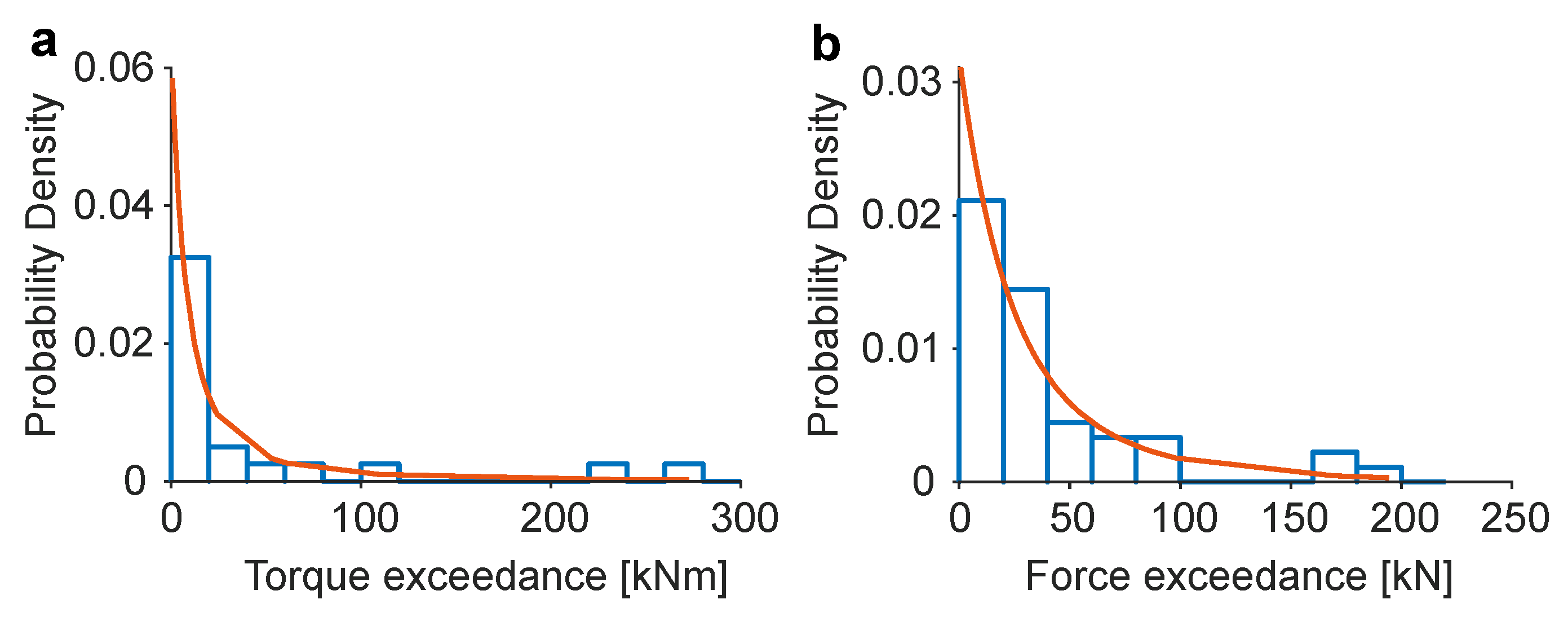
3.2. Fitting the Distribution of Extremes

The GPD distribution was utilized to fit the extremes, while the selection of the threshold involved a combination of a mean excess plot and goodness-of-fit (p-value) analysis performed under various threshold-parameter scenarios. The threshold selection for torque and force amplitude is shown in Figure 7 and Figure 8.
According to the mean excess plot, the threshold should be selected at the inflection point where there is a sharp decrease. However, choosing the threshold at this point may result in a very small number of extreme values, making it difficult to support the fitting of the GPD. Therefore, by considering the relationship between shape and scale parameters and the threshold, as well as the current goodness of fit (p-value), it is possible to select a reasonable threshold. The final threshold for torque was chosen as 79.445 kNm, and for force, it was 160.202 kN. The parameter selection for the GPD is shown in Table 1. The final fitting results are depicted in Figure 9, illustrating the goodness of fit achieved.

3.3. Fitting the Distribution of the Median Amplitude

To model the distribution of the intermediate values using the DKDE method, we took the mean values of the torque and force amplitudes as the minimum values and the threshold as the maximum value. The minimum value, maximum value, bandwidth, and goodness of fit are shown in Table 2. The final fit is shown in Figure 10, where the DKDE distribution perfectly fits the median values of torque and force.

3.4. Load Extrapolation and Damage Evaluation

To extrapolate the load using the ICDF of the fitted distribution, it is necessary to estimate the load values beyond the observed range, allowing predictions based on the characteristics of the fitted distribution to be made. Based on the number of extreme and intermediate values, random numbers are generated within the range of [ 0 , 1 ] . The extrapolation of torque and force amplitudes is illustrated in Figure 11, where Figure 11a,b represent the extrapolation of extreme values, while Figure 11c,d include both extreme and intermediate values.
Moreover, the extrapolation results of different extrapolation methods are compared. Three types of extrapolation methods are compared; namely, parametric extrapolation, linear (proportional) extrapolation, and the proposed non-stationary load extrapolation method. Linear extrapolation extrapolates the original load with a certain number of folds and does not estimate the statistics or distribution of the original load [2]. The method does not take into account large loads that may occur during the life cycle, and the results are biased towards conservatism. The parametric method extrapolates the original load through the estimated mean and amplitude distributions, generally using a Weibull distribution to fit the PDF of the amplitude value and a Gaussian or mixed Gaussian distribution to fit the PDF of the mean value [30].
The cumulative frequency cycle of the extrapolated values can be seen in Figure 12. This plot represents the cumulative probability of the extrapolated torque and force amplitudes over a specified range. Indeed, as depicted in Figure 12, the extrapolation method we employed effectively accounted for the potential occurrence of extreme and moderate load values. This conservative approach is particularly beneficial for structural components, as it considers a wider range of potential loads, ensuring a higher level of safety and reliability. By combining the extrapolated amplitudes with the original mean values, the final extrapolated load spectrum can be created. The nonlinear pseudo-damage of the original load and a tenfold load spectrum obtained with different methods are shown in Table 3.
When parameter extrapolation is applied, the resulting step spectrum may lead to the inclusion of large force loads alongside large torque loads. This can potentially result in excessive damage and may not accurately reflect the actual operating conditions. It is essential to consider the practical aspects of the working environment and the interplay between torque and force loads to ensure a more realistic representation of the damage evolution process. The proposed method of extrapolation resulted in possible extreme and intermediate load values, which led to a extrapolated damage 12.59 times the original load. This conservative estimate demonstrates that the extrapolation approach considers a wider range of potential loads and is more inclined towards a conservative estimation of damage.

4. Conclusions

The drilling pipe of a rotary rig is subject to the dual action of torque and force, which necessitates a rational extrapolation of the load spectrum to enhance structural design and lifespan assessment. However, existing load spectrum extrapolation methods fail to adequately address the challenge of non-stationary load extrapolation with multiple loads acting simultaneously.
To overcome this limitation, we propose a novel load extrapolation framework tailored for the extrapolation of multiple non-stationary loads. Through synchronized rainflow counting, the torque and force loads on the drill pipe are converted into mean-sequence and amplitude-sequence data. Subsequently, the extremes of the amplitude sequence are fitted using the GPD, while the intermediate values are fitted using the DKDE. By employing the estimated parameters and observed data, the ICDF of the fitted distribution can be calculated. Utilizing different probabilities as inputs to the ICDF allows for the determination of corresponding amplitude values, thereby providing insights into potential values that may lie beyond the observed dataset. Finally, the extrapolated amplitude and mean values are combined to form the ultimate load spectrum.
The extrapolation results highlight the efficacy of our proposed method in addressing the challenges posed by multiple non-stationary loads, enabling the extrapolation of possible extreme and intermediate values. Furthermore, the nonlinear cumulative pseudo-damage results demonstrate that our method yields more conservative fatigue damage estimations. Overall, our proposed framework contributes novel insights into the realm of extrapolation of multiple non-stationary loads.

Author Contributions

Conceptualization, H.W. and Z.Z.; methodology, H.W. and Y.S.; software, H.W. and Y.S.; validation, Z.Z. and J.W.; formal analysis, H.W.; investigation, J.Z.; resources, Z.Z. and J.W.; data curation, Z.Z. and J.Z.; writing—original draft preparation, H.W.; writing—review and editing, Y.S. and J.W.; visualization, H.W.; supervision, J.W.; project administration, Z.Z.; funding acquisition, J.W. All authors have read and agreed to the published version of the manuscript.

Funding

This research was funded by the National Natural Science Foundation of China (no. 52272434).

Data Availability Statement

Data are unavailable due to privacy.

Acknowledgments

Thanks to Xuzhou Construction Machinery Group for the promotion of innovation and industrialized application.

Conflicts of Interest

Author Haijin Wang was employed by the company Xuzhou Construction Machinery Group. The remaining authors declare that the research was conducted in the absence of any commercial or financial relationships that could be construed as a potential conflict of interest.

Abbreviations

The following abbreviations are used in this paper:
CDFCumulative Distribution Function
ICDFInverse Cumulative Distribution Function
KDEKernel Density Estimation
DKDEDiffusion Kernel Density Estimation
PDFProbability Density Function
GPDGeneralized Pareto Distribution

References

  1. Lu, X.; Jiang, T. Working Pose Measurement and Quality Evaluation of Rotary Drilling Rig Based on Laser Tracker. Optik 2019, 187, 311–317. [Google Scholar] [CrossRef]
  2. Wang, J.; Chen, H.; Li, Y.; Wu, Y.; Zhang, Y. A Review of the Extrapolation Method in Load Spectrum Compiling. Stroj. Vestn. J. Mech. Eng. 2016, 62, 60–75. [Google Scholar] [CrossRef]
  3. Sun, L.; Liu, M.; Wang, Z.; Wang, C.; Luo, F. Research on Load Spectrum Reconstruction Method of Exhaust System Mounting Bracket of a Hybrid Tractor Based on MOPSO-Wavelet Decomposition Technique. Agriculture 2023, 13, 1919. [Google Scholar] [CrossRef]
  4. Samavatian, V.; Iman-Eini, H.; Avenas, Y. An Efficient Online Time-Temperature-Dependent Creep-Fatigue Rainflow Counting Algorithm. Int. J. Fatigue 2018, 116, 284–292. [Google Scholar] [CrossRef]
  5. Loew, S.; Bottasso, C.L. Lidar-Assisted Model Predictive Control of Wind Turbine Fatigue via Online Rainflow-Counting Considering Stress History. Wind Energ. Sci. 2021, 7, 1605–1625. [Google Scholar] [CrossRef]
  6. Obermayr, M.; Riess, C.; Wilde, J. A Novel Online 4-Point Rainflow Counting Algorithm for Power Electronics. Microelectron. Reliab. 2021, 120, 114112. [Google Scholar] [CrossRef]
  7. Musallam, M.; Johnson, C.M. An Efficient Implementation of the Rainflow Counting Algorithm for Life Consumption Estimation. IEEE Trans. Reliab. 2012, 61, 978–986. [Google Scholar] [CrossRef]
  8. Twomey, J.M.; Chen, D.Y.; Osterman, M.D.; Pecht, M.G. Development of a Cycle Counting Algorithm with Temporal Parameters. Microelectron. Reliab. 2020, 109, 113652. [Google Scholar] [CrossRef]
  9. Zhu, Y.; Zhang, S.; Yan, M. A Cycle Counting Method Considering Load Sequence. Int. J. Fatigue 1993, 15, 407–411. [Google Scholar] [CrossRef]
  10. Jiang, D. A Sequence Retainable Iterative Algorithm for Rainflow Cycle Counting. SAE Int. J. Mater. Manuf. 2014, 7, 108–114. [Google Scholar] [CrossRef]
  11. Jin, T.; Yan, C.; Guo, J.; Chen, C.; Zhu, D. Compilation of Drilling Load Spectrum Based on the Characteristics of Drilling Force. Int. J. Adv. Manuf. Technol. 2022, 124, 4045–4055. [Google Scholar] [CrossRef]
  12. Wang, Y. A Novel Method for the Distribution and Extrapolation of Extreme Sea State Parameters. Ocean Eng. 2022, 251, 111102. [Google Scholar] [CrossRef]
  13. Liu, X.; Wang, H.; Wu, Q.; Wang, Y. Uncertainty-Based Analysis of Random Load Signal and Fatigue Life for Mechanical Structures. Arch. Comput. Methods Eng. 2021, 29, 375–395. [Google Scholar] [CrossRef]
  14. Johannesson, P. Extrapolation of Load Histories and Spectra. Fatigue Fract. Eng. Mater. Struct. 2006, 29, 209–217. [Google Scholar] [CrossRef]
  15. Zheng, G.; Liao, Y.; Chen, B.; Zhao, S.; Wei, H. Multi-Axial Load Spectrum Extrapolation Method for Fatigue Durability of Special Vehicles Based on Extreme Value Theory. Int. J. Fatigue 2024, 178, 108014. [Google Scholar] [CrossRef]
  16. Shangguan, W.B.; Zheng, G.F.; Rakheja, S.; Yin, Z. A method for editing multi-axis load spectrums based on the wavelet transforms. Measurement 2020, 162, 107903. [Google Scholar] [CrossRef]
  17. Poloni, D.; Oboe, D.; Sbarufatti, C.; Giglio, M. Towards a stochastic inverse Finite Element Method: A Gaussian Process strain extrapolation. Mech. Syst. Signal Process. 2023, 189, 110056. [Google Scholar] [CrossRef]
  18. Wen, C.K.; Li, R.C.; Zhao, C.J.; Chen, L.P.; Wang, M.H.; Yin, Y.X.; Meng, Z.J. An improved LSTM-based model for identifying high working intensity load segments of the tractor load spectrum. Comput. Electron. Agric. 2023, 210, 107879. [Google Scholar] [CrossRef]
  19. Lin, P.; Ding, F.; Hu, G.; Li, C.; Xiao, Y.; Tse, K.; Kwok, K.; Kareem, A. Machine learning-enabled estimation of crosswind load effect on tall buildings. J. Wind. Eng. Ind. Aerodyn. 2022, 220, 104860. [Google Scholar] [CrossRef]
  20. Shen, Y.; Zhang, W.; Wang, J.; Feng, C.; Qiao, Y.; Sun, C. A Boom Damage Prediction Framework of Wheeled Cranes Combining Hybrid Features of Acceleration and Gaussian Process Regression. Measurement 2023, 221, 113401. [Google Scholar] [CrossRef]
  21. Yang, G.; Wang, P.; Han, W.; Chen, S.; Zhang, S.; Yuan, Y. Automatic generation of fine-grained traffic load spectrum via fusion of weigh-in-motion and vehicle spatial–temporal information. Comput. Aided Civ. Infrastruct. Eng. 2022, 37, 485–499. [Google Scholar] [CrossRef]
  22. Yang, J.; Kang, G.; Kan, Q. A novel deep learning approach of multiaxial fatigue life-prediction with a self-attention mechanism characterizing the effects of loading history and varying temperature. Int. J. Fatigue 2022, 162, 106851. [Google Scholar] [CrossRef]
  23. Botev, Z.I.; Grotowski, J.F.; Kroese, D.P. Kernel Density Estimation via Diffusion. Ann. Stat. 2010, 38, 2916–2957. [Google Scholar] [CrossRef]
  24. Ma, S.; Sun, S.; Wang, B.; Wang, N. Estimating Load Spectra Probability Distributions of Train Bogie Frames by the Diffusion-Based Kernel Density Method. Int. J. Fatigue 2020, 132, 105352. [Google Scholar] [CrossRef]
  25. Marsh, G.; Wignall, C.; Thies, P.R.; Barltrop, N.; Incecik, A.; Venugopal, V.; Johanning, L. Review and Application of Rainflow Residue Processing Techniques for Accurate Fatigue Damage Estimation. Int. J. Fatigue 2016, 82, 757–765. [Google Scholar] [CrossRef]
  26. Wang, Q.; Zhou, J.; Gong, D.; Wang, T.; Sun, Y. Fatigue Life Assessment Method of Bogie Frame with Time-Domain Extrapolation for Dynamic Stress Based on Extreme Value Theory. Mech. Syst. Signal Process. 2021, 159, 107829. [Google Scholar] [CrossRef]
  27. Shen, Y.; Li, X.; Wang, J.; Liu, C.; Kong, W. An Extrapolation Framework for Torque Spectrum of Excavator Internal Combustion Engine via Bivariate Diffusion-Based Kernel Density Estimation. Proc. Inst. Mech. Eng. Part C J. Mech. Eng. Sci. 2023, 237, 133–147. [Google Scholar] [CrossRef]
  28. Peng, Z.; Huang, H.Z.; Zhou, J.; Li, Y.F. A New Cumulative Fatigue Damage Rule Based on Dynamic Residual S-N Curve and Material Memory Concept. Metals 2018, 8, 456. [Google Scholar] [CrossRef]
  29. Johannesson, P.; Speckert, M. Guide to Load Analysis for Durability in Vehicle Engineering; John Wiley & Sons: Hoboken, NJ, USA, 2013. [Google Scholar] [CrossRef]
  30. Liu, X.; Zhang, M.; Wang, H.; Luo, J.; Tong, J.; Wang, X. Fatigue Life Analysis of Automotive Key Parts Based on Improved Peak-over-threshold Method. Fatigue Fract. Eng. Mater. Struct. 2020, 43, 1824–1836. [Google Scholar] [CrossRef]
Figure 1. Schematic diagram of load on drill pipe. (a) Rotation torque and applied force acting on the drill pipe. (b) Time history of rotation torque and applied force.
Machines 12 00075 g001
Figure 2. Multiple non-stationary load extrapolation framework.
Machines 12 00075 g002
Figure 3. Turning point (TP) filter and hysteresis (rainflow) filter.
Machines 12 00075 g003
Figure 4. Load testing of drill pipe on rotary drilling rig.
Machines 12 00075 g004
Figure 5. Torque (a) and force (b) of drill pipe before (blue) and after (red) data preprocessing.
Machines 12 00075 g005
Figure 6. Simultaneous rainflow count results. (a) Torque amplitude and sequence, (b) torque mean and sequence, (c) torque rainflow matrix, (d) force amplitude and sequence, (e) force mean and sequence, and (f) force rainflow matrix.
Machines 12 00075 g006
Figure 7. The threshold selection for the force amplitude sequence, where the red lines are the error boundary and the blue line is the ture value. (a) Mean excess, (b) threshold shape parameter, (c) threshold scale parameter, and (d) threshold p-value.
Machines 12 00075 g007
Figure 8. The threshold selection for the force amplitude sequence, where the red lines are the error boundary and the blue line is the ture value. (a) Mean excess, (b) threshold shape parameter, (c) threshold scale parameter, and (d) threshold p-value.
Machines 12 00075 g008
Figure 9. GPD fit for extremes, where the red lines are the error boundary and the blue line is the ture value. (a) Torque extremes, (b) force extremes.
Machines 12 00075 g009
Figure 10. DKDE fit for median values. (a) Torque median values, (b) force median values.
Machines 12 00075 g010
Figure 11. Load extrapolation for amplitude sequence. (a) Extreme extrapolation of torque amplitude, (b) extreme extrapolation of force amplitude, (c) load extrapolation of torque amplitude, and (d) load extrapolation of force amplitude.
Machines 12 00075 g011
Figure 12. Cumulative frequency of cycles for load extrapolation. (a) Torque amplitude extrapolation, (b) force amplitude extrapolation.
Machines 12 00075 g012
Table 1. The parameter selection for the GPD.
ItemsShape ParameterScale ParameterThresholdp-ValueNumber of Extremes
Torque amplitude−1.00515.40979.445 kNm0.58833
Force amplitude−0.26931.233160.202 kN0.83545
Table 2. The parameter for the fitted DKDE.
ItemsMinimum ValueMaximum ValueBandwidthGoodness of FitNumber of Median Values
Torque amplitude15.392 kNm79.445 kNm0.9720.9942706
Force amplitude32.494 kN160.202 kN2.0300.9952371
Table 3. Comparison of nonlinear pseudo-damage of original load and tenfold load spectrum.
ItemsNonlinear Pseudo-DamageRatio
Original load 2.25 × 10 13 1.00
Parametric extrapolation 5.33 × 10 14 20.90
Liner extrapolation 2.64 × 10 14 10.35
Proposed extrapolation 3.21 × 10 14 12.59
Disclaimer/Publisher’s Note: The statements, opinions and data contained in all publications are solely those of the individual author(s) and contributor(s) and not of MDPI and/or the editor(s). MDPI and/or the editor(s) disclaim responsibility for any injury to people or property resulting from any ideas, methods, instructions or products referred to in the content.

