Article

Multi-Condition Intelligent Fault Diagnosis Based on Tree-Structured Labels and Hierarchical Multi-Granularity Diagnostic Network

1
The School of Electrical Technology, Guangdong Mechanical and Electrical Polytechnic, Guangzhou 510515, China
2
The School of Mechanical and Automotive Engineering, South China University of Technology, Guangzhou 510641, China
*
Author to whom correspondence should be addressed.
Machines 2024, 12(12), 891; https://doi.org/10.3390/machines12120891
Submission received: 4 November 2024 / Revised: 28 November 2024 / Accepted: 4 December 2024 / Published: 6 December 2024
(This article belongs to the Special Issue AI-Driven Reliability Analysis and Predictive Maintenance)

Abstract

:
The aim of this study is to improve the cross-condition domain adaptability of bearing fault diagnosis models and their diagnostic performance under previously unknown conditions. Thus, this paper proposes a multi-condition adaptive bearing fault diagnosis method based on multi-granularity data annotation. A tree-structured labeling scheme is introduced to allow for multi-granularity fault annotation. A hierarchical multi-granularity diagnostic network is designed to automatically learn multi-level fault information from condition data using feature extractors of varying granularity, allowing for the extraction of shared fault information across conditions. Additionally, a multi-granularity fault loss function is developed to help the deep network learn tree-structured labels, improving intra-class compactness and reducing hierarchical similarity between classes. Two experimental cases demonstrate that the proposed method exhibits robust cross-condition domain adaptability and performs better in unseen conditions than state-of-the-art methods.

1. Introduction

Bearings are critical components in mechanical equipment and play an essential role in modern industrial production. The complex and variable working environments put a significant strain on bearing lifespan. When combined with the high-load and high-speed operating characteristics, these conditions exacerbate bearing failures and damage [1,2], resulting in mechanical equipment breakdowns. Severe equipment failures in modern manufacturing are leading causes of safety incidents, economic losses, and even fatalities [3]. Therefore, timely and reliable fault diagnosis of bearings is crucial.
With the widespread use of the Industrial Internet of Things (IIoT) [4] and deep learning [5,6], numerous data-driven methods for fault diagnosis have emerged by extracting fault features from sensor signals [7]. These methods primarily rely on operational data from equipment under specific working conditions, with the assumption that data features are consistent between the training and testing phases [8]. However, in practice, the variability of working conditions often results in significant differences in data features across operating conditions, resulting in severe data distribution shifts between the source domain (training domain) and the target domain (testing domain) [9]. Consequently, models trained under one condition cannot be directly applied to other conditions, resulting in a significant drop in diagnostic performance [10].
In recent years, techniques such as transfer learning [11,12], generative adversarial networks (GANs) [13,14], and deep autoencoders [15,16,17] have received attention for addressing cross-condition diagnostic challenges. These methods attempt to improve model adaptability by reducing the distribution discrepancy between different working conditions using techniques such as feature mapping and domain alignment. However, these approaches primarily focus on improving diagnostic performance by modifying network architecture [18], whereas optimization from the perspective of data annotation to improve diagnostic accuracy is relatively unknown. Further study is required to improve cross-condition fault diagnosis performance using data annotation strategies.
In summary, existing fault diagnosis methods’ cross-condition domain adaptability needs to be improved further. To address this issue, this paper proposes an intelligent fault diagnosis method based on tree-structured labeling (TSL) and a hierarchical multi-granularity diagnostic network (HMDN). The main contributions of this study are as follows:
(1)
A novel TSL method is proposed for creating multi-granularity fault labels that provide deep networks with more detailed fault attribute information.
(2)
An HMDN is designed to perform multi-granularity signal analysis, extracting fault information at multiple levels within a single condition. This improves the model’s ability to automatically identify common fault features in new conditions, resulting in greater adaptability across domains.
(3)
A multi-granularity fault loss function is developed to assist the model in learning fine-grained information while also extracting detailed features, even when using low-quality, coarse-grained labels.
The remainder of this paper is organized as follows. Section 2 summarizes the current state of relevant research. Section 3 describes the TSL method and the HMDN. Section 4 evaluates the effectiveness of the proposed method using two experimental cases. Finally, Section 5 concludes the paper.

2. Related Work

Cross-condition fault diagnosis of bearings is an important technology for addressing the challenges of multi-condition intelligent maintenance in complex equipment [19,20]. Current research mainly focuses on improving the network architecture to improve feature alignment across different working conditions.
For instance, Zhu et al. [21] proposed an adaptive multi-scale convolutional manifold embedding network that addresses distribution discrepancies in various condition data by designing intra- and inter-class constraints. Shi et al. [22] proposed the Adversarial Multi-source Data Subdomain Adaptation (AMDSA) model, which addresses multi-domain adaptation issues in heterogeneous multi-source data using subdomain adaptation strategies and feature fusion mechanisms. Jia et al. [23] proposed a Causal Disentanglement Domain Generalization (CDDG) method for fault diagnosis that improves cross-domain diagnostic performance by reconstructing shared features across condition domains. Chen et al. [24] proposed a novel zero-shot learning method for bearing fault diagnosis (BFD) in multiple unknown domains, which recognizes fault types in different conditions using common fault attributes. Xing et al. [25] developed a full-domain adaptive periodic cyclic sparse network for deep transfer fault diagnosis of rolling bearings, transferring knowledge learned in the source domain to the target domain through repeated training on target domain data, resulting in cross-condition fault diagnosis. Xiao et al. [26] proposed a joint transfer network for unsupervised bearing fault diagnosis from the simulation field to the experimental field. By improving the loss function, the cross-domain marginal distribution and conditional distribution can be aligned simultaneously in the unsupervised scenario.
In summary, most current studies focus on improving network structures through adversarial generation and autoencoders to create consistent features across different conditions. However, no studies have yet investigated using multi-granularity labeling to extract multidimensional features from condition data. As a result, there is an urgent need to develop a multi-granularity labeling approach to assist networks in extracting multi-level features from data, thereby improving fault diagnosis in new working conditions.

3. Proposed TLSs and HMDN

Figure 1 depicts the intelligent fault diagnosis process using tree-structured labels (TSLs) and an HMDN. First, data collection and labeling are carried out. Sensors collect mechanical fault data, which are then cleaned and segmented before assigning TSLs. The labeled data are then passed to the HMDN for model training. The network is optimized using a combined loss function that combines the tree-structured loss and the multi-class cross-entropy loss. Finally, the model’s performance on the test dataset is evaluated using ablation studies, comparative experiments, and confusion matrix analysis.

3.1. Subsection

In engineering practice, data often have multiple attributes, and a single label may not fully capture the rich features of the data. For example, in natural language processing, a document may contain multiple topics, whereas in image recognition, an image may contain multiple objects. Hierarchical labeling, which progresses from coarse to fine granularity, can better express the multidimensional features found in data. However, such labeling necessitates expert involvement or specialized training, which makes it time-consuming and labor-intensive. As a result, in practical applications, only specific tasks are labeled, resulting in underutilization of available data.
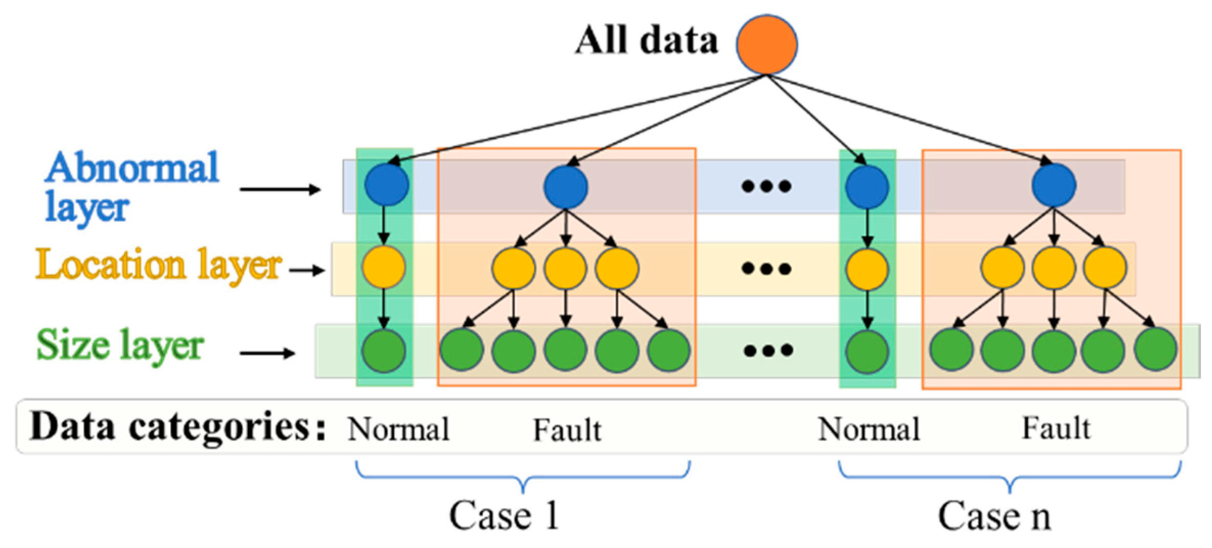
When analyzing cross-condition fault datasets, mechanical fault data can be labeled at various levels, including defect type, location, and size. For instance, the “12k_Drive_End_B007_0_118” data under the 0 hp condition from the Case Western Reserve University (CWRU) dataset can be decomposed into “defect, ball-defect, 0.007-inch,” resulting in hierarchical labels at the defect type, location, and size levels. A single data point is thus labeled hierarchically, capturing information from coarse to fine granularity. Each hierarchical label is represented by a 0–1 vector, with different sections denoting different levels of information. The label vectors for all data points in the dataset form a label tree, which is traversed breadth-first to generate the label vector for each data point. Figure 2 illustrates how this TSL method expresses the dependencies and relationships between various data points.
Further definitions of the TSL approach are provided as follows. The TSLs T = ( N , E h , E e ) consist of a set of nodes N = ( n 1 , n 2 , n 3 , , n m ) , directed edges E h V × V , and undirected edges E m V × V . Each node n N corresponds to a different class label. The number of nodes m is equal to the number of all labels in the tree structure. The directed edge ( v i , v j ) E h is an inclusion edge, indicating that label i contains label j . For example, “fault” under 0 hp is the parent or superclass of “ball bearing fault”. The undirected edge ( v i , v j ) E e is an exclusion edge, indicating that classes v i and v j are mutually exclusive. For example, in the CWRU dataset, all faults are single faults, which indicates that a fault sample cannot be both a “ball bearing fault” and an “inner ring fault” simultaneously. Any two nodes can share inclusion and exclusion edges.
Each class label takes a binary value, v i { 0,1 } , to indicate whether the data sample belongs to that class. Then, each edge specifies the constraints under which the two labels of its associated nodes can take binary values. It is prohibited to assign ( v i , v j ) = ( 0,1 ) to the inclusion edge ( v i , v j ) E h (for example, “ball bearing failure” but not “fault”). It is also illegal to assign ( v i , v j ) = ( 1,1 ) to the exclusion edge ( v i , v j ) E e (for example, both “ball bearing failure” and “inner race failure”). All inclusion and exclusion edges are defined by these local constraints. The binary label vector y { 0,1 } m represents the legal global assignment of all labels. The set of all legal global assignments forms the state space S T { 0,1 } m of the tree. The state space S T is a matrix of size R ( m + 1 ) × m , with each row representing a legal binary label vector y .

3.2. Tree-Structured Loss

To effectively incorporate hierarchical label information into the model, a composite loss function is created, which combines the tree-structured loss and the multi-class cross-entropy loss. The tree-structured loss is designed to convey hierarchical knowledge during training. In practical industrial scenarios, samples with leaf-node annotations are often limited; thus, the tree-structured classification loss may struggle to distinguish fine-grained classes at the leaf level. To address this, the weight of the fine-grained classification loss is increased, with the multi-class cross-entropy loss reinforcing the leaf classes’ mutual exclusivity constraints.
The derivation of the tree-structured loss is as follows. Assume there are m sigmoid nodes, each of which corresponds to a TSL node and represents a class label. The binary labels assigned to each class form a label vector y i . Given an input fault signal, the joint probability of all sigmoid output nodes with respect to the label vector can be calculated using the following equation:
P ~ ( y | x ) = i = 1 m ϕ i ( x ~ i , y i ) i , j { 1 , , n } ψ i , j ( y ~ i , y ~ j ) .
where x ~ i represents the sigmoid output of the i -th label node and P ~ ( y | x ) denotes the probability without normalization. The calculation formula of ϕ i ( x ~ i , y i ) is ϕ i x ~ i , y i = e x ~ i y i = 1 , and ψ i , j ( y i , y j ) represents the constraint defined in the TSLs between any two labels in y , which is defined as follows:
ψ i , j ( y i , y j ) = 0 ,   E x c l u s i o n   c o n s t r a i n t 1 ,   I n c l u s i o n   c o n s t r a i n t .
Then, the joint probability is normalized as Pr ( y , x ) = P ~ ( y | x ) Z ( x ) , where Z ( x ) is the partition function for all legal assignments y ~ S T in the state space of the tree-structured label T , defined as follows:
Z ( x ) = y ~ { 0,1 } m i = 1 m ϕ i ( x ~ i , y i ) i , j { 1 , , n } ψ i , j ( y ~ i , y ~ j ) .
For the input fault signal x , after the model inference output, the output tree hierarchy can be compared with the TSLs to obtain all legal assignments of y i = 1 , and the marginal probability Pr ( y i = 1 | x ) of label i can be obtained by summing them up. The calculation formula is as follows:
Pr ( y i = 1 | x ) = 1 Z ( x ) y ~ : y ~ i = 1 i ϕ i ( x ~ i , y ~ i ) i , j ψ i , j ( y ~ i , y ~ j ) .
The marginal probability of a leaf node in the TSLs (T) is determined by the sum of its ancestral scores, because if the leaf node’s label is 1, then all of its ancestors must also be 1, allowing the parent node’s score to influence the offspring’s decision. On the other hand, the parent label’s marginal probability is marginalized over all possible states of its offspring, aggregating information from all of its subclasses.
During training, the input label may be at any level of the tree hierarchy, and the training objective is to maximize the marginal probability of the observed true label. Given k training samples D = { x ( l ) , y ( l ) , g ( l ) } , l = 1,2 , , k , where g ( l ) { 1,2 , , k } represents the index of the observed label, the probability classification loss, that is, the tree structure loss, is shown as follows:
L t r e e ( D ) = 1 k l = 1 k ln ( Pr ( y g ( l ) ( l ) = 1 | x ( l ) ) ) .
To further improve the ability to distinguish fine-grained leaf categories, the model incorporates a multi-class cross-entropy loss L c e based on the tree structure loss. The model includes a parallel softmax output layer that infers and outputs fine-grained leaf categories, with each node representing a fine-grained leaf label in the TSLs. The activation of softmax ensures mutual exclusion between fine-grained leaf classes, which corresponds to the TSLs’ mutual exclusion constraints. The tree structure loss and the multi-class cross-entropy loss are combined to form a joint loss. The joint loss for a single sample is defined as follows:
L c o m b ( x ( l ) , y g ( l ) ( l ) ) = L c e + L t r e e ,   g ( l )   i s   a   l e a f   n o d e L t r e e ,   o t h e r .
Depending on whether x ( l ) is marked as a fine-grained leaf category, we can choose whether to introduce the multi-classification cross-entropy loss L c e according to the formula, and then the total loss of k samples in the dataset D is obtained as follows:
L t o t a l ( D ) = 1 k l = 1 k L c o m b ( x ( l ) , y g ( l ) ( l ) ) .

3.3. Structural Design of HMDN

As shown in Figure 3, the HMDN consists of a global feature extractor, a hierarchical feature interaction module, and two parallel output channels. To handle one-dimensional data, the global feature extractor uses a modified ResNet18_1D, which extracts features from the input signal.
The hierarchical feature interaction module consists of feature extraction blocks with specific granularity and shortcut connections. Each specific-granularity feature extraction block is made up of two convolutional layers and two fully connected (FC) layers that extract dedicated features from various hierarchical levels. The residual connections linearly combine the features of finer subcategories with those of coarser superclasses, allowing subcategories to inherit superclass features while also retaining their own unique features. A nonlinear transformation (ReLU) is then applied to the combined features to capture generalized nonlinear characteristics.
The model is equipped with two output channels. The first output channel calculates a probabilistic classification loss based on the TSLs, with each sigmoid node representing a different label in the hierarchy. Sigmoid activation functions are used to reflect independent relationships and organize the hierarchical nodes based on structural constraints. The second output channel computes multi-class cross-entropy loss for the leaf nodes, reinforcing the mutual exclusivity of fine-grained classes during training.
Using this architecture, the HMDN efficiently learns multi-level fault information from input data, extracting both coarse- and fine-grained features, resulting in improved fault diagnosis performance across a range of operational conditions.

4. Case Studies

4.1. Case 1: Paderborn University Dataset

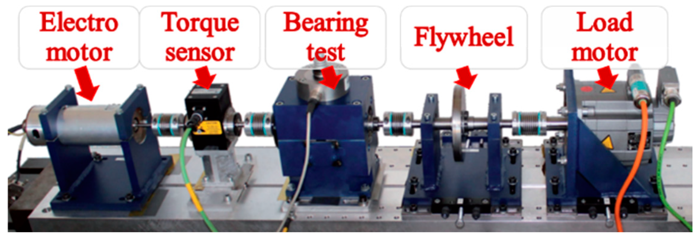
Paderborn University’s (PU) bearing dataset [27] includes both artificially induced and naturally occurring bearing faults. Figure 4 depicts the experimental setup, with data collected using a piezoelectric accelerometer sensor at a sampling rate of 64 kHz. The experiments cover four operating conditions: driving speed, radial force, load torque, and other variations.
The PU dataset contains 32 sets of experimental data, including 12 artificially damaged bearings, 14 bearings with accelerated wear damage, and six sets of healthy bearing data under various operating conditions. For this study, one healthy and eight faulty conditions are selected, with details provided in Table 1 and Table 2.
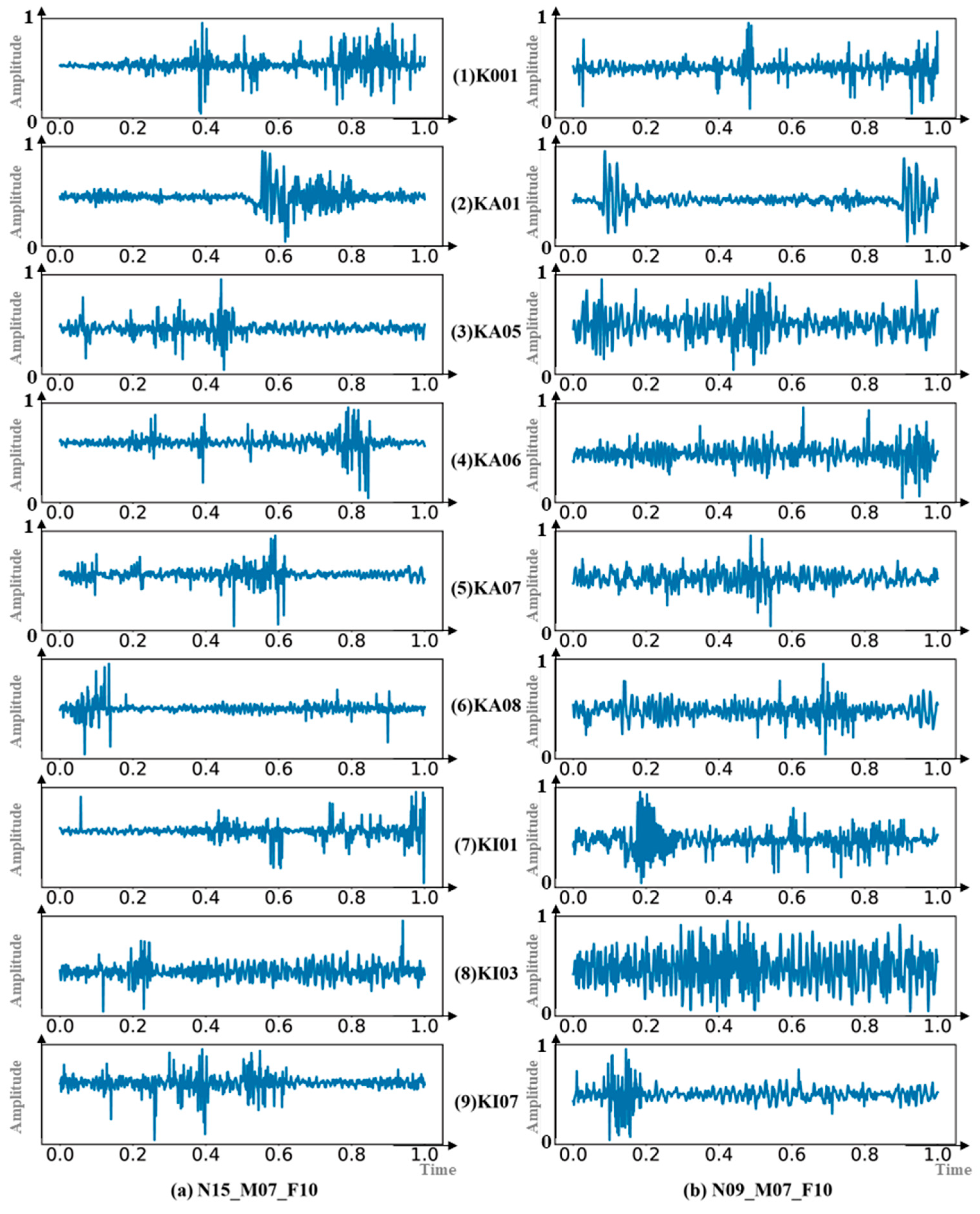
A total of 36 datasets were created from nine different health states under four operating conditions. The datasets were augmented using a sliding window technique and divided into segments of 800 samples per set (1024 × 1), totaling 28,800 samples. These samples were labeled using the TSL method and served as the dataset for this study. A total of 70% (20,160 samples) of the data were randomly selected for training, with the remaining 30% (8640 samples) selected for testing. Figure 5 shows examples of data under the N15_M07_F10 and N09_M07_F10 conditions, demonstrating that there are significant differences between fault types, whereas data from the same fault type across different conditions show minimal variation.
Furthermore, to simulate scenarios in which detailed labeling is lacking, different proportions (0%, 30%, 50%, 70%, and 90%) of training samples had their fine-grained subclass labels (fault size) reassigned to their immediate parent class (fault location). These proportions are referred to as the re-labeling ratio (proportion). In contrast, the test set evaluated samples with the full hierarchical label structure.
By structuring the dataset in this manner, we were able to test the proposed method’s robustness when faced with incomplete or less detailed annotations during the training phase, while still retaining fully labeled data for analysis. This setup allows for a better understanding of the method’s adaptability and performance across different annotation quality levels.

4.2. Evaluation Metrics

To evaluate the performance of the HMDN on the PU dataset, two key evaluation metrics were used:
(1)
Hierarchical Accuracy: The HMDN model generates probabilities for each class. The predicted label is determined by selecting the class with the highest probability at each level, and the hierarchical accuracy is calculated on the test set. Specifically, three levels of accuracy are measured: Acc-abnormal (accuracy in detecting abnormalities), Acc-location (accuracy in identifying fault locations), and Acc-size (accuracy in classifying fault sizes). This metric evaluates the model’s classification performance across multiple hierarchical levels.
(2)
Area Under the Precision–Recall Curve (AUPRC): AUPRC is calculated by averaging the Precision–Recall Curves (PRC) for all classes and evaluating the output probability vectors at each hierarchical level. The advantage of AUPRC is its independence from specific classification thresholds, which reduces the error rate caused by thresholds that are manually set. For a given threshold, a point (precision Pre and recall Rec) on the PRC curve is calculated as follows:
P r e = i = 1 n T P i i = 1 n T P i + i = 1 n F P i R e c = i = 1 n T P i i = 1 n T P i + i = 1 n F N i
where i represents all classes, and T P i , F P i , and F N i denote the true positives, false positives, and false negatives for class i , respectively. By adjusting the threshold, the PRC curve is generated, and the area under this curve (AUPRC) is calculated.

4.3. Model Training

The proposed model used a combined loss function that included a tree-structured loss and a categorical cross-entropy loss, which was optimized with the SGD optimizer. The learning rate was set to 0.0001, momentum to 0.9, weight decay to 0.0005, and batch size to 32, yielding a total of 200 training iterations. The learning rate was adjusted using a cosine annealing algorithm. To reduce the effect of random variation, the experiments were repeated five times for each network.
The experiment in this paper is conducted on an I7-10400 CPU and an RTX3060 graphics card, with a 16 G personal computer used for training and testing purposes.

4.4. Ablation Studies on HMDN

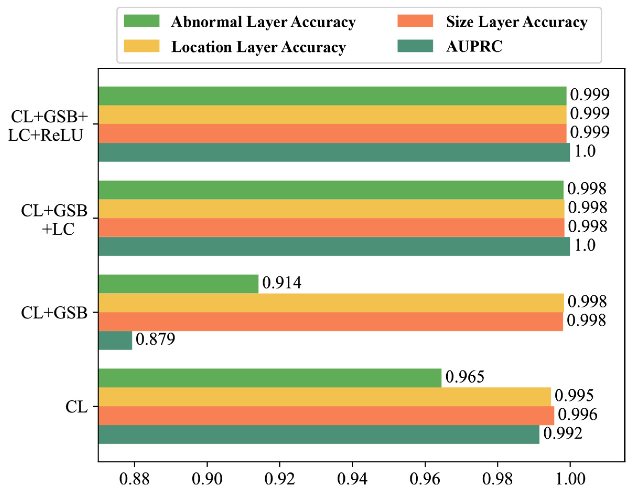
Ablation studies are conducted to determine the contributions of various components in the model. As shown in Figure 6, the HMDN is made up of the following modules: (1) Granularity-specific Block (GSB): Extracts features specific to various granularities. (2) Linear Combination (LC): Combines hierarchical features using residual connections. (3) ReLU: Performs a nonlinear transformation on the combined features.
The base model, which only included ResNet18_1D and the combined loss (CL), achieved a fault size accuracy of 99.2%. However, after the GSB module was implemented, performance dropped, possibly due to overfitting caused by increased network complexity. By incorporating the LC module, performance improved above that of the CL-only model, indicating that feature fusion contributes to better overall performance. Finally, the ReLU module improved the model’s generalization ability by mapping linear features into a more robust nonlinear space.

4.5. Ablation Study on Loss Functions

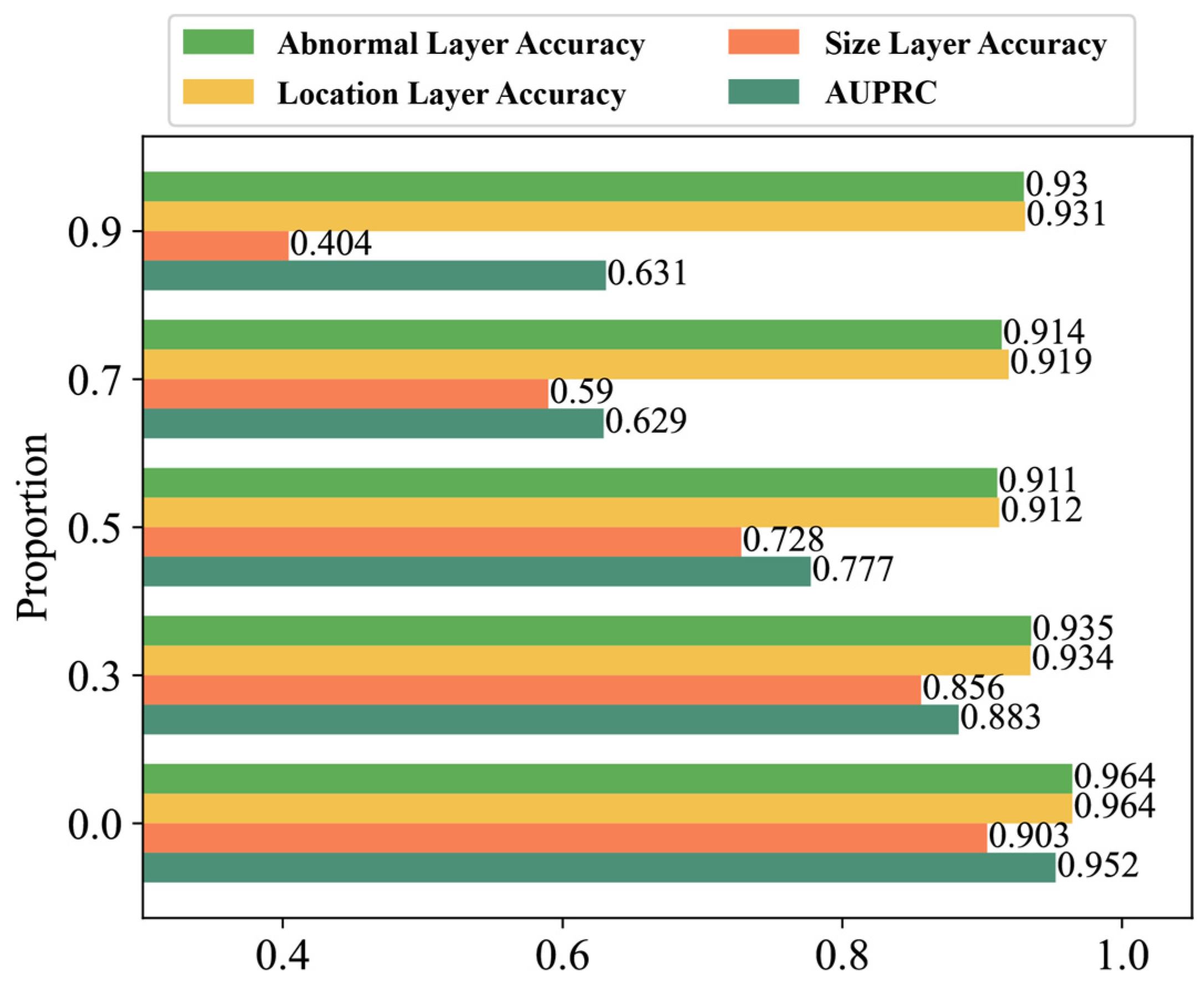
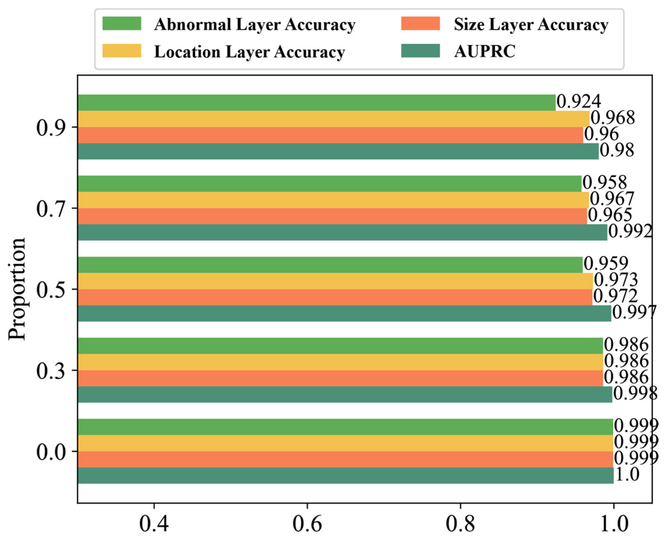
The effectiveness of the combined loss function L c o m b (which combines tree-structured loss L t r e e and categorical cross-entropy loss L c e ) was verified through additional ablation studies (see Figure 7 and Figure 8). Across various relabeling proportions (0%, 30%, 50%, 70%, and 90%), models trained with the combined loss L c o m b consistently outperformed those using only the tree-structured loss L t r e e .
Furthermore, as more training samples were relabeled to coarse-grained classes, the fine-grained classification performance of the model with L t r e e deteriorated significantly. In contrast, by applying L c e to the fine-grained leaf nodes, the combined loss L c o m b consistently outperformed L t r e e . For example, when the relabeling rate reached 90%, the combined loss was more than twice as accurate at the fine-grained fault size level as the tree-structured loss model.

4.6. Comparative Analysis with SOTA Methods

To demonstrate the superiority of HMDN, this section compares it to three state-of-the-art (SOTA) models: MTACNN [28], MTAGN [29], and WDCNN [30]. In these experiments, the output layers of MTACNN, MTAGN, and WDCNN were changed to correspond to three hierarchical levels: defect type, fault location, and fault size. The experiments were conducted under varying relabeling ratios across all methods. The analysis is primarily concerned with the fine-grained size level accuracy, which contains more detailed information than the coarse-grained defect and location levels. The coarse-grained levels can be derived from the fine-grained levels, making the latter more important.
As shown in Figure 9, a multi-classification loss function was applied at each hierarchical level, and the total loss was calculated by adding the losses at all three levels. Because no hierarchical training strategy was explicitly designed, relabeled samples were discarded during training to ensure label consistency across hierarchical levels in MTACNN, MTAGN, and WDCNN. Furthermore, versions of these models that employed a combined loss strategy—MTACNN(CL), MTAGN(CL), and WDCNN(CL)—replaced the sum of the cross-entropy loss functions with a combined loss function as the total loss.
The results in Figure 9 demonstrate that HMDN consistently outperforms all other models for all five relabeling ratios. Moreover, as the relabeling ratio increases, HMDN’s performance degrades at a much slower rate than MTACNN, MTAGN, and WDCNN, which all experience significant drops. Notably, the performance of MTACNN(CL), MTAGN(CL), and WDCNN(CL) with combined loss outperforms their non-combined loss counterparts across all relabeling ratios. Additionally, the performance degradation in these models with combined loss becomes less severe as the relabeling ratio increases.
This demonstrates that the combined loss approach effectively uses samples with shallow label information during model training, whereas a small number of samples with deep label information can further optimize the model. Using the combined loss, the training data can be fully exploited, reducing data loss and improving overall model performance.

4.7. Case 2: Triple-GB Dataset

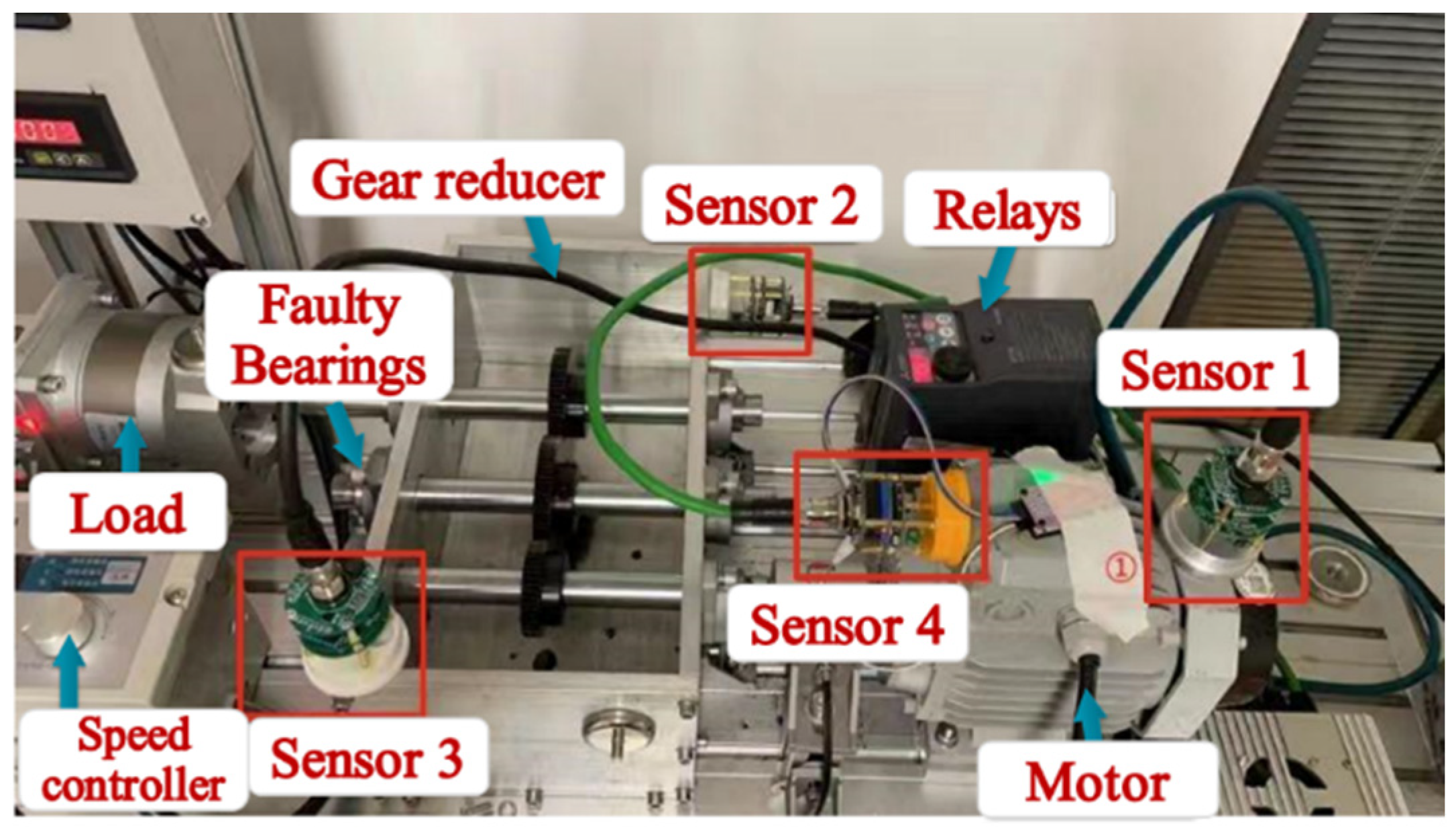
In our lab, an experimental platform called the Triple Gear Bearing Experiment Platform (Triple-GB) is constructed, which included three gears and three pairs of bearings, as shown in Figure 10. The platform consists of a motor, motor speed controller, relay, drive shaft, supporting bearings, gearbox, load, test bearings, and four sensors.
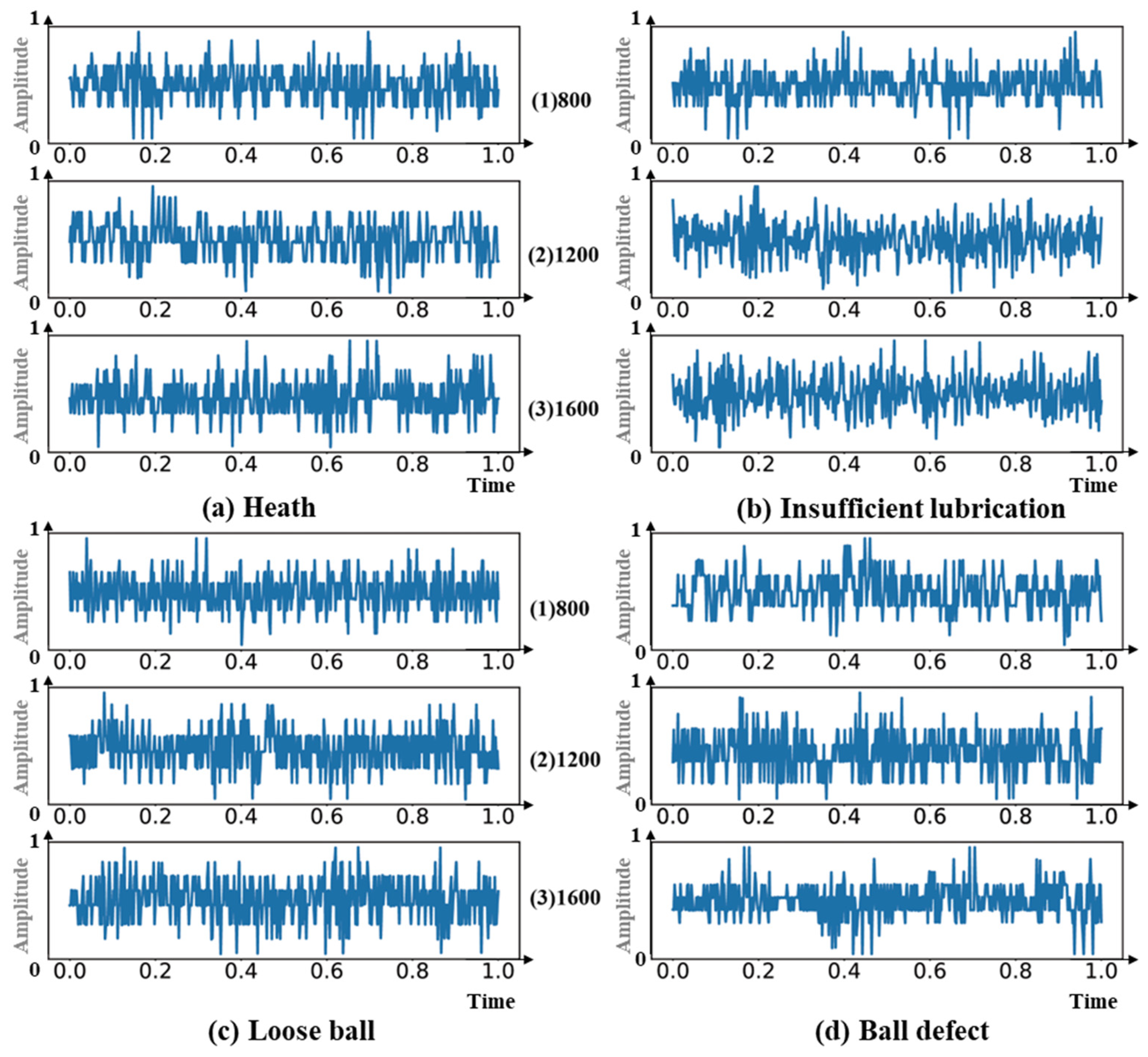
Four fault types were considered: healthy, insufficient lubrication, loose ball, and ball defect, with three operating conditions: 800, 1200, and 1600 RPM, yielding a total of twelve datasets. The data were segmented using a window size of 2048, with each set containing 1000 samples, for a total of 12,000 samples. The dataset was randomly divided into 70% training and 30% test sets. Figure 11 shows sample data collected by sensor 3 from the 12 groups.

4.8. Comparative Analysis with SOTA Models

A comparative experiment between HMDN and three other models was conducted on the Triple-GB dataset. Table 3 presents the results for hierarchical accuracy at higher relabeling ratios (0.7 and 0.9). It is clear that HMDN consistently achieved the highest accuracy for both defect and location levels across various relabeling ratios while maintaining relatively stable performance. Furthermore, when compared to the standard cross-entropy loss models of MTACNN, MTAGN, and WDCNN, the models with the combined loss function outperformed the others in terms of accuracy and stability. At a relabeling ratio of 0.9, HMDN outperformed WDCNN in hierarchical accuracy by over 20%, both with and without the combined loss function.
Compared to the previous case study results, HMDN’s performance metrics improved in this section, indicating that the fault features in the Triple-GB dataset are more pronounced and easier to extract and distinguish than those in the PU dataset. This can also be due to the Triple-GB dataset’s relatively low number of fault types and operating conditions.
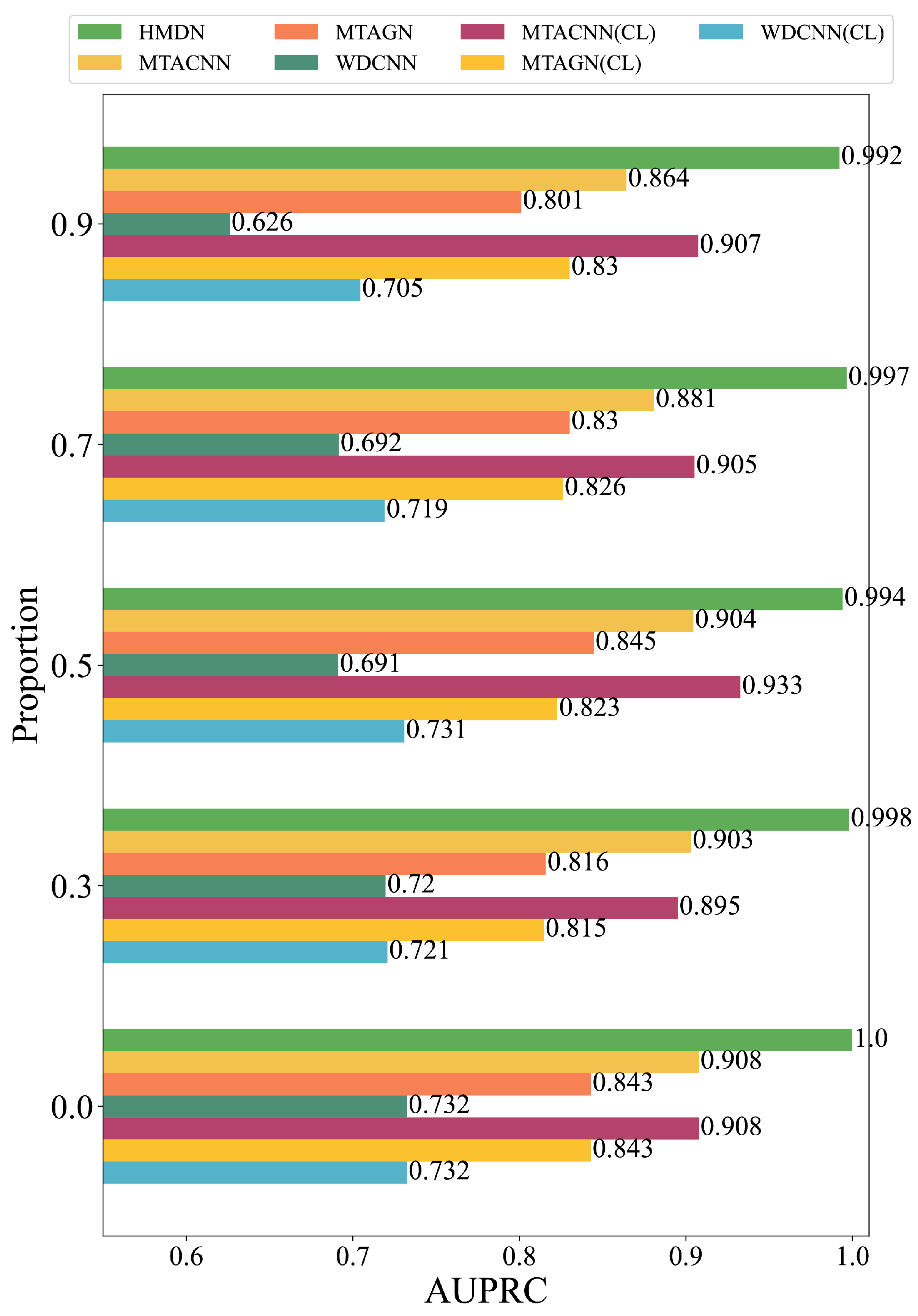
To further evaluate the model’s performance across different recall rates, the Area Under the Precision–Recall Curve (AUPRC) metric was employed, which comprehensively considers precision and recall across varying thresholds. Figure 12 shows the results. HMDN not only had the best AUPRC score, but it also showed remarkable stability as the relabeling ratio increased. From a relabeling ratio of 0.0 to 0.9, the AUPRC score decreased by only 0.008. MTACNN outperformed the other models in terms of AUPRC, but there was still a more than 10% gap between them and HMDN. This indicates that HMDN can maintain strong performance across different classification thresholds, which is useful for dealing with imbalanced class scenarios and other challenging classification tasks.

4.9. Confusion Matrix Visualization Analysis

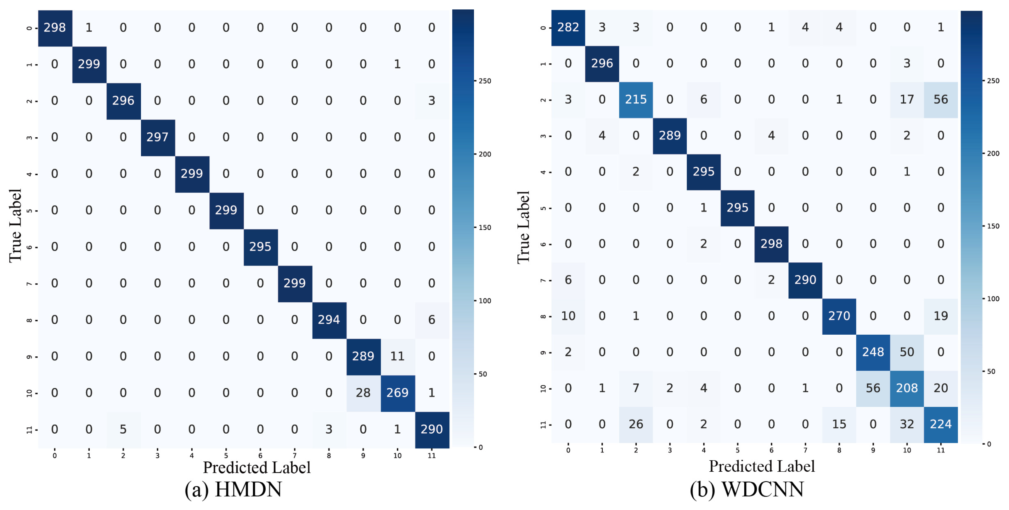
To reveal differences in performance across fine-grained categories, a confusion matrix experiment was carried out for both HMDN and WDCNN with a relabeling ratio of 0.7, as shown in Figure 13 and Figure 14. At the defect level, HMDN outperformed WDCNN in all fine-grained categories, with the main differences occurring in the fault types under three different operating conditions. At the location level, HMDN and WDCNN performed similarly in the majority of categories, with HMDN slightly outperforming WDCNN overall. Additionally, WDCNN demonstrated significant misclassification in categories 9–11 (i.e., the healthy condition was misidentified as bearing defects), resulting in lower overall performance.

4.10. Feature Distribution Visualization

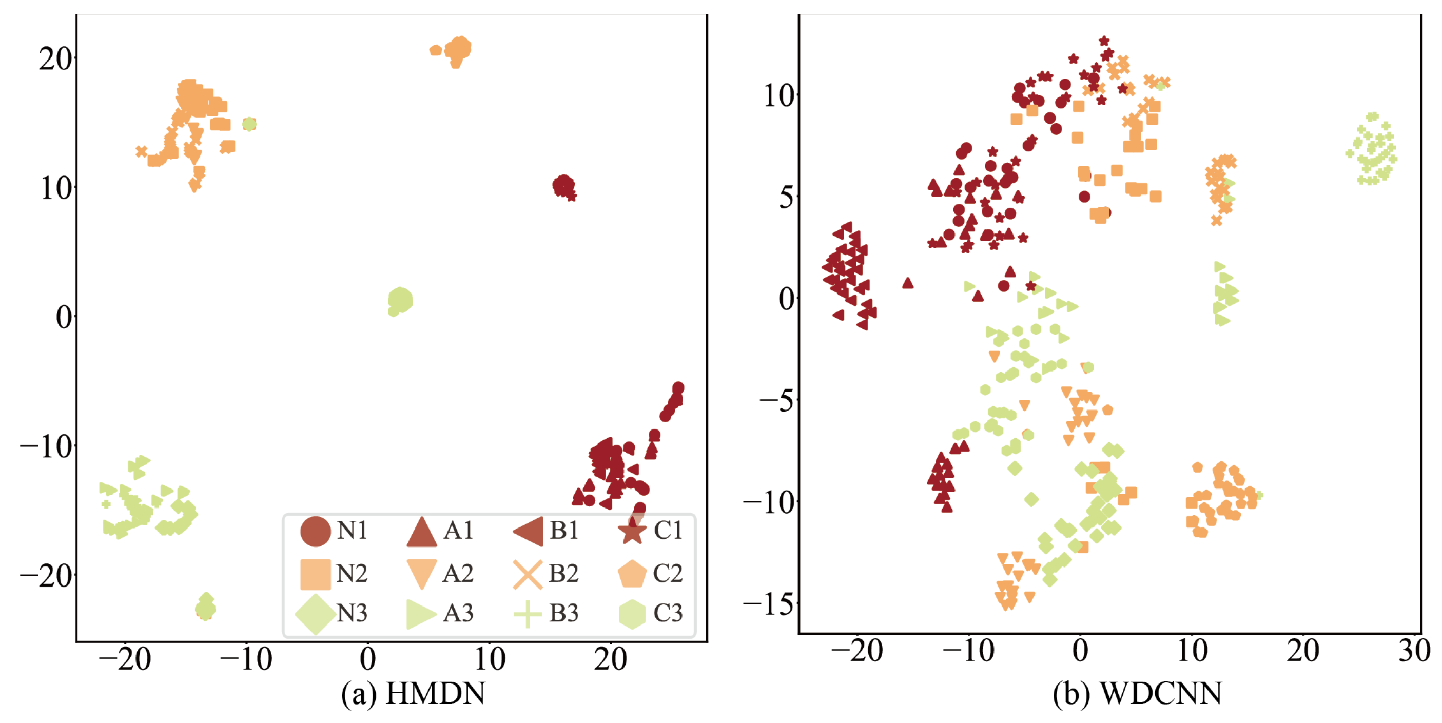
This section visualizes the feature distributions of HMDN and WDCNN using t-SNE for the output of the final layer with a relabeling ratio of 0.9, as shown in Figure 15. The HMDN visualization shows a clear separation between the clusters of different colors, indicating that HMDN effectively extracted and distinguished features associated with various operating conditions. Moreover, within the same operating condition, fault features were well-clustered, with minimal intra-class distance, but inter-class separation could be improved.
In contrast, WDCNN, which was used as the control model in this study, struggled to distinguish between operating condition features, and its fault features were scattered, indicating weaker feature extraction and aggregation capabilities compared to HMDN.

5. Conclusions

This paper proposes an intelligent fault diagnosis algorithm that integrates TSLs with an HMDN to address the challenges of unstable performance and insufficient granularity in fault data annotation under multiple operating conditions. Initially, the original annotation data were analyzed to produce hierarchical labels with granularities ranging from coarse to fine. These parsed labels were then represented as a hierarchical 0–1 label vector, resulting in a label tree. The HMDN was then trained and optimized using a combined loss function that included a tree-structured loss as well as a multi-class cross-entropy loss. The tree-structured loss encodes semantic relationships between any two levels of labels, allowing for cross-hierarchical knowledge transfer, whereas the multi-class cross-entropy loss improves discriminative capability for leaf-level categories. The HMDN uses shortcut connections to encourage hierarchical feature interaction. Comprehensive experiments were carried out on the PU dataset and the Triple-GB platform. The results demonstrate that the proposed HMDN effectively addresses the issue of poor data labeling quality under a variety of operating conditions, achieving higher diagnostic accuracy than existing methods.

Author Contributions

Conceptualization, J.T. and Y.L.; methodology, Y.L.; resources, H.Y. and J.W.; writing—original draft preparation, J.T.; writing—review and editing, J.T. and H.Y.; visualization, H.Y.; supervision, S.W.; project administration, S.W.; funding acquisition, J.W. All authors have read and agreed to the published version of the manuscript.

Funding

The Natural Science Foundation of Guangdong Province, China (No. 2024A1515012009), The Guangdong Basic and Applied Basic Research Foundation (No. 2022A1515240061).

Data Availability Statement

The data presented in this study are available on request from the corresponding author due to privacy.

Conflicts of Interest

The authors declare no conflicts of interest.

References

  1. Lei, Z.; Shi, J.; Luo, Z.; Cheng, M.; Wan, J. Intelligent Manufacturing from the Perspective of Industry 5.0: Application Review and Prospects. IEEE Access 2024, 12, 167436–167451. [Google Scholar] [CrossRef]
  2. Huang, K.; Zhu, L.; Ren, Z.; Lin, T.; Zeng, L.; Wan, J.; Zhu, Y. An Improved Fault Diagnosis Method for Rolling Bearings Based on 1D_CNN Considering Noise and Working Condition Interference. Machines 2024, 12, 383. [Google Scholar] [CrossRef]
  3. Tan, J.; Wan, J.; Chen, B.; Safran, M.; AlQahtani, S.A.; Zhang, R. Selective Feature Reinforcement Network for Robust Remote Fault Diagnosis of Wind Turbine Bearing Under Non-Ideal Sensor Data. IEEE Trans. Instrum. Meas. 2024, 73, 3515911. [Google Scholar] [CrossRef]
  4. Chettri, L.; Bera, R. A Comprehensive Survey on Internet of Things (IoT) Toward 5G Wireless Systems. IEEE Internet Things J. 2020, 7, 16–32. [Google Scholar] [CrossRef]
  5. Wan, J.; Li, X.; Dai, H.N.; Kusiak, A.; Martínez-García, M.; Li, D. Artificial-Intelligence-Driven Customized Manufacturing Factory: Key Technologies, Applications, and Challenges. Proc. IEEE 2021, 109, 377–398. [Google Scholar] [CrossRef]
  6. Ali, N.; Wang, Q.; Gao, Q.; Ma, K. Diagnosis of Multicomponent Faults in SRM Drives Based on Auxiliary Current Reconstruction Under Soft-Switching Operation. IEEE Trans. Ind. Electron. 2024, 71, 2265–2276. [Google Scholar] [CrossRef]
  7. Yan, S.; Shao, H.; Xiao, Y.; Liu, B.; Wan, J. Hybrid robust convolutional autoencoder for unsupervised anomaly detection of machine tools under noises. Robot. Comput.-Integr. Manuf. 2023, 79, 102441. [Google Scholar] [CrossRef]
  8. Gao, Q.; Huang, T.; Zhao, K.; Shao, H.; Jin, B. Multi-source weighted source-free domain transfer method for rotating machinery fault diagnosis. Expert Syst. Applications 2024, 237, 121585. [Google Scholar] [CrossRef]
  9. Guo, S.; Zhang, B.; Yang, T.; Lyu, D.; Gao, W. Multitask Convolutional Neural Network with Information Fusion for Bearing Fault Diagnosis and Localization. IEEE Trans. Ind. Electron. 2020, 67, 8005–8015. [Google Scholar] [CrossRef]
  10. Zhang, M.; Wang, D.; Lu, W.; Yang, J.; Li, Z.; Liang, B. A Deep Transfer Model with Wasserstein Distance Guided Multi-Adversarial Networks for Bearing Fault Diagnosis Under Different Working Conditions. IEEE Access 2019, 7, 65303–65318. [Google Scholar] [CrossRef]
  11. Hu, Q.; Si, X.; Qin, A.; Lv, Y.; Liu, M. Balanced Adaptation Regularization Based Transfer Learning for Unsupervised Cross-Domain Fault Diagnosis. IEEE Sens. J. 2022, 22, 12139–12151. [Google Scholar] [CrossRef]
  12. Tian, J.; Han, D.; Li, M.; Shi, P. A multi-source information transfer learning method with subdomain adaptation for cross-domain fault diagnosis. Knowl.-Based Syst. 2022, 243, 108466. [Google Scholar] [CrossRef]
  13. Kuang, J.; Xu, G.; Tao, T.; Wu, Q.; Han, C.; Wei, F. Domain Conditioned Joint Adaptation Network for Intelligent Bearing Fault Diagnosis Across Different Positions and Machines. IEEE Sens. J. 2023, 23, 4000–4010. [Google Scholar] [CrossRef]
  14. Xu, J.; Li, K.; Fan, Y.; Yuan, X. A label information vector generative zero-shot model for the diagnosis of compound faults. Expert Syst. Appl. 2023, 233, 120875. [Google Scholar] [CrossRef]
  15. Li, B.; Zhao, C. Federated Zero-Shot Industrial Fault Diagnosis with Cloud-Shared Semantic Knowledge Base. IEEE Internet Things J. 2023, 10, 11619–11630. [Google Scholar] [CrossRef]
  16. Zhang, L.; Zhang, H.; Cai, G. The Multiclass Fault Diagnosis of Wind Turbine Bearing Based on Multisource Signal Fusion and Deep Learning Generative Model. IEEE Trans. Instrum. Meas. 2022, 71, 3514212. [Google Scholar] [CrossRef]
  17. Wen, L.; Gao, L.; Li, X. A New Deep Transfer Learning Based on Sparse Auto-Encoder for Fault Diagnosis. IEEE Trans. Syst. Man Cybern. Syst. 2019, 49, 136–144. [Google Scholar] [CrossRef]
  18. Zhang, X.; He, C.; Lu, Y.; Chen, B.; Zhu, L.; Zhang, L. Fault diagnosis for small samples based on attention mechanism. Measurement 2022, 187, 110242. [Google Scholar] [CrossRef]
  19. Xia, M.; Li, T.; Shu, T.; Wan, J.; de Silva, C.W.; Wang, Z. A Two-Stage Approach for the Remaining Useful Life Prediction of Bearings Using Deep Neural Networks. IEEE Trans. Ind. Inform. 2019, 15, 3703–3711. [Google Scholar] [CrossRef]
  20. He, M.; Li, Z.; Hu, F. A Novel RUL-Centric Data Augmentation Method for Predicting the Remaining Useful Life of Bearings. Machines 2024, 12, 766. [Google Scholar] [CrossRef]
  21. Zhu, X.; Zhao, X.; Yao, J.; Deng, W.; Shao, H.; Liu, Z. Adaptive Multiscale Convolution Manifold Embedding Networks for Intelligent Fault Diagnosis of Servo Motor-Cylindrical Rolling Bearing Under Variable Working Conditions. IEEE/ASME Trans. Mechatron. 2024, 29, 2230–2240. [Google Scholar] [CrossRef]
  22. Shi, J.; Wang, X.; Lu, S.; Zheng, J.; Dong, H.; Zhang, J. An Adversarial Multisource Data Subdomain Adaptation Model: A Promising Tool for Fault Diagnosis of Induction Motor Under Cross-Operating Conditions. IEEE Trans. Instrum. Meas. 2023, 72, 3519014. [Google Scholar] [CrossRef]
  23. Jia, L.; Chow, T.W.S.; Yuan, Y. Causal Disentanglement Domain Generalization for time-series signal fault diagnosis. Neural Netw. 2024, 172, 106099. [Google Scholar] [CrossRef] [PubMed]
  24. Chen, Z.; Wu, J.; Deng, C.; Wang, X.; Wang, Y. Deep Attention Relation Network: A Zero-Shot Learning Method for Bearing Fault Diagnosis Under Unknown Domains. IEEE Trans. Reliab. 2023, 72, 79–89. [Google Scholar] [CrossRef]
  25. Xing, Z.; Yi, C.; Lin, J.; Zhou, Q. A Novel Periodic Cyclic Sparse Network with Entire Domain Adaptation for Deep Transfer Fault Diagnosis of Rolling Bearing. IEEE Sens. J. 2023, 23, 13452–13468. [Google Scholar] [CrossRef]
  26. Xiao, Y.; Shao, H.; Han, S.; Huo, Z.; Wan, J. Novel Joint Transfer Network for Unsupervised Bearing Fault Diagnosis From Simulation Domain to Experimental Domain. IEEE/ASME Trans. Mechatron. 2022, 27, 5254–5263. [Google Scholar] [CrossRef]
  27. Lessmeier, C.; Kimotho, J.K.; Zimmer, D.; Sextro, W. Condition Monitoring of Bearing Damage in Electromechanical Drive Systems by Using Motor Current Signals of Electric Motors: A Benchmark Data Set for Data-Driven Classification. In Proceedings of the European Conference of the Prognostics and Health Management Society, Bilbao, Spain, 5–8 July 2016. [Google Scholar]
  28. Shao, S.; Yan, R.; Lu, Y.; Wang, P.; Gao, R.X. DCNN-Based Multi-Signal Induction Motor Fault Diagnosis. IEEE Trans. Instrum. Meas. 2020, 69, 2658–2669. [Google Scholar] [CrossRef]
  29. Woo, S.; Park, J.; Lee, J.-Y.; Kweon, I.S. CBAM: Convolutional Block Attention Module. In Computer Vision—ECCV 2018, Proceedings of the 15th European Conference, Munich, Germany, 8–14 September 2018; Ferrari, V., Hebert, M., Sminchisescu, C., Weiss, Y., Eds.; Springer International Publishing: Cham, Switzerland, 2018; pp. 3–19. [Google Scholar]
  30. Guo, Q.; Li, Y.; Song, Y.; Wang, D.; Chen, W. Intelligent Fault Diagnosis Method Based on Full 1-D Convolutional Generative Adversarial Network. IEEE Trans. Ind. Inform. 2020, 16, 2044–2053. [Google Scholar] [CrossRef]
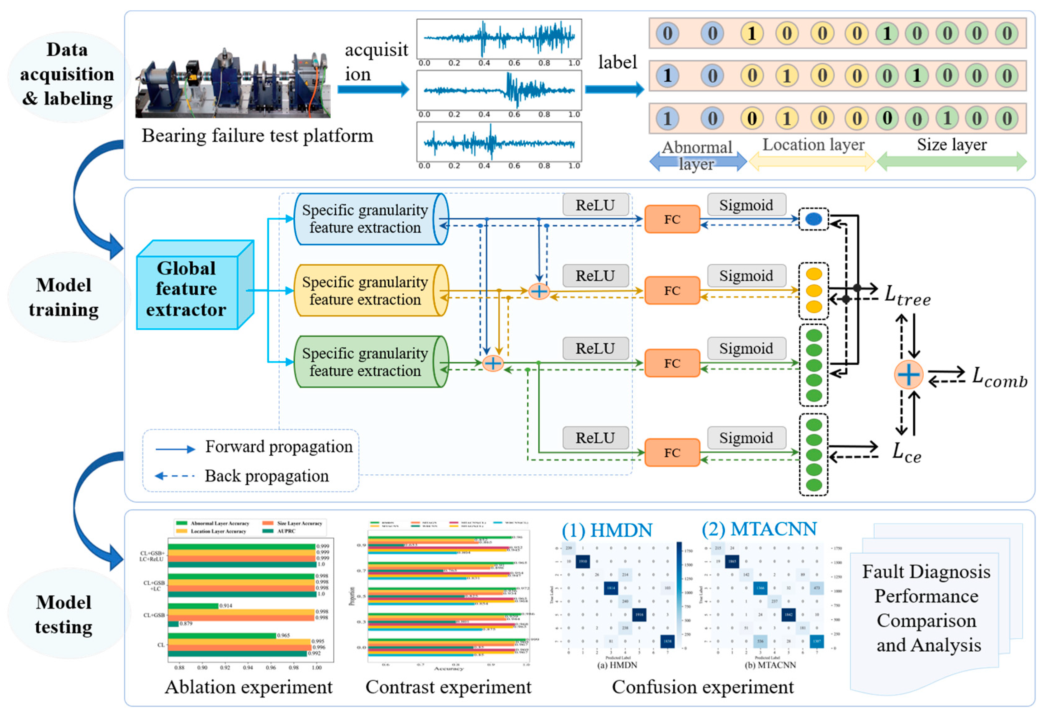
Figure 1. Intelligent fault diagnosis flow based on tree labels and hierarchical multi-granularity diagnosis network.
Machines 12 00891 g001
Figure 2. Logical diagram of the TSL method.
Machines 12 00891 g002
Figure 3. Schematic diagram of HMDN.
Machines 12 00891 g003
Figure 4. Bearing failure test bench for the PU dataset.
Machines 12 00891 g004
Figure 5. Example data from the PU dataset under the N15_M07_F10 and N09_M07_F10 conditions.
Machines 12 00891 g005
Figure 6. Model performance in the ablation study for the deep learning architecture.
Machines 12 00891 g006
Figure 7. Performance of the model using tree-structured loss.
Machines 12 00891 g007
Figure 8. Performance of the model using the combined loss.
Machines 12 00891 g008
Figure 9. Fine-grained size level accuracy in the comparative experiments.
Machines 12 00891 g009
Figure 10. Self-built Triple-GB experimental platform.
Machines 12 00891 g010
Figure 11. Example of data collected by sensor 3 in Triple-GB dataset.
Machines 12 00891 g011
Figure 12. AUPRC results of the model under different relabeling rates.
Machines 12 00891 g012
Figure 13. Confusion matrix for the defect level in the Triple-GB dataset.
Machines 12 00891 g013
Figure 14. Confusion matrix for the location level in the Triple-GB dataset.
Machines 12 00891 g014
Figure 15. t-SNE visualization of the feature distribution for the location level in the Triple-GB dataset.
Machines 12 00891 g015
Table 1. Experimental conditions in the PU dataset.
LabelSpeed (rpm)Load Torque (Nm)Radial Force (N)Annotation Information
WC115000.71000N15_M07_F10
WC29000.71000N09_M07_F10
WC315000.11000N15_M01_F10
WC415000.7400N15_M07_F04
Table 2. Annotation information for nine health data types in the PU dataset.
LabelIDDefect PresentFault LocationCause of DefectFault Severity Level
NormalK001NONoneNoneNone
OR-EDMKA01YesInner RingElectrical Discharge Machining1
OR-EE1KA05YesInner RingElectric Engraving1
OR-EE1KA06YesInner RingElectric Engraving2
OR-Drill1KA07YesInner RingDrilling1
OR-Drill2KA08YesInner RingDrilling2
IR-EDMKI01YesOuter RingElectrical Discharge Machining1
IR-EE1KI03YesOuter RingElectric Engraving1
IR-EE2KI07YesOuter RingElectric Engraving2
Table 3. Performance of HMDN and other models on the Triple-GB dataset.
ProportionModelAbnormalLocation
AccStdAccStd
0.7MTACNN97.44420.0136797.44420.01367
MTAGN97.05350.0136797.24880.01367
WDCNN90.06130.0370289.49210.02845
MTACNN(CL)98.24210.0370297.69530.01367
MTAGN(CL)97.44970.0136797.47760.01367
WDCNN(CL)95.41290.0223294.49770.04464
HMDN98.58250.0111698.33140.01116
0.9MTACNN95.51890.0136795.79790.01367
MTAGN95.83140.0223295.64730.03056
WDCNN78.47650.0284579.27450.02734
MTACNN(CL)97.94080.0111697.32140.01367
MTAGN(CL)97.30460.0136796.96420.01116
WDCNN(CL)93.98990.0136790.65840.02734
HMDN98.80240.0136798.29570.01116
Disclaimer/Publisher’s Note: The statements, opinions and data contained in all publications are solely those of the individual author(s) and contributor(s) and not of MDPI and/or the editor(s). MDPI and/or the editor(s) disclaim responsibility for any injury to people or property resulting from any ideas, methods, instructions or products referred to in the content.