


Localization and Mapping for Self-Driving Vehicles: A Survey

 , ,
, ,  , ,
, ,
Abstract
1. Introduction
- Comprehensively reviewing the feature extraction methods in the field of autonomous driving.
- Providing clear details on what are the solutions to create a map for autonomous vehicles, by investigating the solutions that use pre-built maps, which can be pre-existing commercial maps or generated by some academic solutions, or the online map solution, which creates a map in the same time with the positioning process.
- Providing necessary background information and demonstrating many existing solutions to solve the localization and mapping tasks.
- Reviewing and analysing localization approaches that exist in the literature together with the related solutions to ensure data security.
- Exploring the environmental footprint and impact of self-driving vehicles in relation to localization and mapping techniques and unveiling solutions for this.
2. Feature Extraction
2.1. Semantic Features
2.2. Non-Semantics Features
2.3. Deep Learning Features
- MixedCNN-based Methods: Convolutional Neural Network (CNN) is one of the most common methods used in computer vision. These types of methods use mathematical operations called ’convolution’ to extract relevant features [62]. VeloFCN [63] is a projection-based method and one of the earliest methods that uses CNN for 3D vehicle detection. The authors used a three convolution layer structure to down-sample the input front of the view map, then up-sample with a deconvolution layer. The output of the last procedure is fed into a regression part to create a 3D box for each pixel. Meanwhile, the same results were entered for classification to check if the corresponding pixel was a vehicle or not. Finally, they grouped all candidates’ boxes and filtered them by a Non-Maximum Suppression (NMS) approach. In the same vein, LMNet [64] increased the zone of detection to find road objects by taking into consideration five types of features: reflectance, range, distance, side, height. Moreover, they change the classical convolution by the dilated ones. The Voxelnet [65] method begins with the process of voxelizing the set of points cloud and passing it through the VFE network (explained below) to obtain robust features. After that, a 3D convolutional neural network is applied to group voxels features into a 2D map. Finally, a probability score is calculated using an RPN (Region Proposal Network). The VFE network aims to learn features of points by using a multi-layer-perceptron and a max-pooling architecture to obtain point-wise features. This architecture concatenates features from the MLP output and the MLP + Maxpooling. This process is repeated several times to facilitate the learning. The last iteration is fed to an FCN to extract the final features. BirdNet [66] generates a three-channel bird eye’s view image, which encodes the height, intensity, and density information. After that, a normalization was performed to deal with the inconsistency of the laser beams of the LiDAR devices. BirdNet uses a VGG16 architecture to extract features, and they adopt a Fast-RCNN to perform object detection and orientation. BirdNet+ [67] is an extension of the last work, where they attempted to predict the height and vertical position of the centroid object in addition to the processing of the source (BirdNet) method. This field is also approached by transfer learning, like in Complex-YOLO [68], and YOLO3D [69]. Other CNN-based method include regularized graph CNN (RGCNN) [70], Pointwise-CNN [71], PointCNN [72], Geo-CNN [73], Dynamic Graph-CNN [74] and SpiderCNN [75].
- Other Methods: These techniques are based on different approaches. Ref. [76] is a machine learning-based method where the authors try to voxelize the set of points cloud into 3D grid cells. They extract features just from the non-empty cells. These features are a vector of six components: mean and variance of the reflectance, three shape factors, and a binary occupancy. The authors proposed an algorithm to compute the classification score, which takes in the input of a trained SVM classification weight and features, then a voting procedure is used to find the scores. Finally, a non-maximum suppression (NMS) is used to remove duplicate detection. Interesting work is done in [77], who tried to present a new architecture of learning that directly extracts local and global features from the set of points cloud. The 3D object detection process is independent of the form of the points cloud. PointNet shows a powerful result in different situations. PointNet++ [78] extended the last work of PointNet, thanks to the Furthest Point Sampling (FPS) method. The authors created a local region by clustering the neighbor point and then applied the PointNet method in each cluster region to extract local features. Ref. [79] introduces a novel approach using LiDAR range images for efficient pole extraction, combining geometric features and deep learning. This method enhances vehicle localization accuracy in urban environments, outperforming existing approaches and reducing processing time. Publicly released datasets support further research and evaluation. The research presents PointCLIP [80], an approach that aligns CLIP-encoded point clouds with 3D text to improve 3D recognition. By projecting point clouds onto multi-view depth maps, knowledge from the 2D domain is transferred to the 3D domain. An inter-view adapter improves feature extraction, resulting in better performance in a few shots after fine-tuning. By combining PointCLIP with supervised 3D networks, it outperforms existing models on datasets such as ModelNet10, ModelNet40 and ScanObjectNNN, demonstrating the potential for efficient 3D point cloud understanding using CLIP. PointCLIP V2 [81] enhances CLIP for 3D point clouds, using realistic shape projection and GPT-3 for prompts. It outperforms PointCLIP [80] by , , and accuracy in zero-shot 3D classification. It extends to few-shot tasks and object detection with strong generalization. Code and prompt details are provided. The paper [82] presents a "System for Generating 3D Point Clouds from Complex Prompts and proposes an accelerated approach to 3D object generation using text-conditional models. While recent methods demand extensive computational resources for generating 3D samples, this approach significantly reduces the time to 1–2 min per sample on a single GPU. By leveraging a two-step diffusion model, it generates synthetic views and then transforms them into 3D point clouds. Although the method sacrifices some sample quality, it offers a practical tradeoff for scenarios, prioritizing speed over sample fidelity. The authors provide their pre-trained models and code for evaluation, enhancing the accessibility of this technique in text-conditional 3D object generation. Researchers have developed 3DALL-E [83], an add-on that integrates DALL-E, GPT-3 and CLIP into the CAD software, enabling users to generate image-text references relevant to their design tasks. In a study with 13 designers, the researchers found that 3DALL-E has potential applications for reference images, renderings, materials and design considerations. The study revealed query patterns and identified cases where text-to-image AI aids design. Bibliographies were also proposed to distinguish human from AI contributions, address ownership and intellectual property issues, and improve design history. These advances in textual referencing can reshape creative workflows and offer users faster ways to explore design ideas through language modeling. The results of the study show that there is great enthusiasm for text-to-image tools in 3D workflows and provide guidelines for the seamless integration of AI-assisted design and existing generative design approaches. The paper [84] introduces SDS Complete, an approach for completing incomplete point-cloud data using text-guided image generation. Developed by Yoni Kasten, Ohad Rahamim, and Gal Chechik, this method leverages text semantics to reconstruct surfaces of objects from incomplete point clouds. SDS Complete outperforms existing approaches on objects not well-represented in training datasets, demonstrating its efficacy in handling incomplete real-world data. Paper [85] presents CLIP2Scene, a framework that transfers knowledge from pre-trained 2D image-text models to a 3D point cloud network. Using a semantics-based multimodal contrastive learning framework, the authors achieve annotation-free 3D semantic segmentation with significant mIoU scores on multiple datasets, even with limited labeled data. The work highlights the benefits of CLIP knowledge for understanding 3D scenes and introduces solutions to the challenges of unsupervised distillation of cross-modal knowledge.
2.4. Discussion
- Time and energy cost: being easy to detect and easy to use in terms of compilation and execution.
- Representativeness: detecting features that frequently exist in the environment to ensure the matching process.
- Accessibility: being easy to distinguish from the environment.
2.5. Challenges and Future Directions
- Features should be robust against any external effect like weather changes, other moving objects, e.g., trees that move in the wind.
- Provide the possibility of re-use in other tasks.
- The detection system should be capable to extract features even with a few objects in the environment.
- The proposed algorithms to extract features should not hurt the system by requiring long execution time.
- One issue that should be taken into consideration is about safe and dangerous features. Each feature must provide a degree of safety (expressed as percentage), which helps to determine the nature of the feature and where they belong to, e.g., belonging to the road is safer than being on the walls.

| Paper | Features Type | Concept | Methods | Features-Extracted | Time and Energy Cost | Representativeness | Accessibility | Robustness |
|---|---|---|---|---|---|---|---|---|
| [21,22], [33,36], [37,38]. | - Semantic | - General | - Radon transform - Douglas & Peukers algorithm - Binarization - Hough transform - Iterative-End- Point-Fit (IEPF) - RANSAC | - Road lanes - lines - ridges Edges - pedestrian crossings lines | - Consume a lot | - High | - Hard | - Passable |
| [24,25], [33]. | - Semantic | - General | - The height of curbs between 10 cm and 15 cm - RANSAC | - Curves | - Consume a lot | - High | - Hard | - Passable |
| [26,27], [28,29], [30,31], [32,33], [40]. | - Semantic | - Probabilistic - General | - Probabilistic Calculation - Voxelisation | - Building facades - Poles | - Consume a lot | - Middle | - Hard | - Low |
| [42,43], [44,46], [47,48], [51,52], [53,54], [49,55], [56,57], [58,59], [60]. | - Non-Semantic | - General | - PCA - DAISY - Gaussian kernel - K-medoids - K-means - DBSCAN - RANSAC - Radius Outlier Removal filter - ORB - BRIEFFAST-9 | - All the environment | - Consume less | - High | - Easy | - High |
| [61,62], [63,64], [65,66], [67,68], [69,70], [71,72], [73,74], [75,76], [77,78]. | - Deep-learning | - Probabilistic - Optimization - General | - CNN - SVM - Non-Maximum Suppression - Region Proposal Network - Multi Layer Perceptron - Maxpooling - Fast-RCNN - Transfer learning | - All the environment | - Consume a lot | - High | - Easy | - High |
3. Mapping
3.1. Offline Maps
- Global accuracy: (Absolute accuracy) position of features according to the face of the earth.
- Local accuracy: (Relative accuracy) position of features according to the surrounding elements on the road.
3.2. Online Maps
| Map | Original Country | Description/Key Features |
|---|---|---|
| Here is one of the companies that provides HD maps solutions and promise its clients to ensure | ||
| the safety and get the driver truth by providing relevant information to offer vehicles more option | ||
| HERE | Netherlands | and to decide comfortably. Here uses machine learning to validate map data against |
| the real-word in the real-time, this technology achieve around 10–20 cm of the accuracy in the | ||
| identification of the vehicles and their surrounding. Moreover, this map contains three | ||
| main layers Road Model, HD Lane Model, and HD Localisation Model [98,99]. | ||
| Support many applications in an (ADAS) like Hans-free driving, advanced lane guidance, lane split, | ||
| curves speed warning, etc. Also, provide a high precise vehicle positioning with an accuracy of 1m | ||
| Tomtom | Netherlands | or better compared to reality and 15 cm in the relative accuracy. Also, Tomtom take the advantage |
| of using the RoadDNA where it converts the 3D points cloud into a 2D raster image which made | ||
| it much easier to implement in-vehicles. Tomtom consist of three-layer | ||
| Navigation data, Planning data, RoadDNA [100,101]. | ||
| Sanborn | USA | Exploit the data received from different sensors Cameras, LiDAR to generate a high-precise 3D base-map. |
| This map attain 7–10 cm of the absolute accuracy [102]. | ||
| Ushr use only stereo camera imaging techniques to reduce the cost of acquiring data, and they use advanced | ||
| Ushr | USA/Japan | machine vision and machine learning enable to achieve 90% of automation of data processing, |
| also this map has mapped over 200,000 miles under 10 cm level of absolute accuracy [103]. | ||
| NVIDIA map detect semantics road features and provides information about vehicles position with | ||
| NVIDIA | USA | robustness and centimeter-level of accuracy. Also, NVIDIA offers the possibility to build and update |
| a map using sensors available on the car [104]. | ||
| Waymo affirmed that a map for (AV) contain much more information than the traditional one and deserve | ||
| to have a continuous maintain and update, due to its complexity and the huge amount of data received. | ||
| Waymo | USA | Waymo extract relevant features on the road from LiDAR sensor, which help to accurately find |
| the vehicle position by matching the real-time features with the pre-built map features, | ||
| this map attains a 10 cm of accuracy without using a GPS [99]. | ||
| Zenrin is one of the leaders’ companies in the creation of map solution in japan, founded in 1948 | ||
| Zenrin | Japan | and has subsidiaries worldwide in Europe, America, and Asia. The company adopt |
| the Original Equipment Manufacturers (OEM) for the automobile industry. Zenrin offer 3D digital | ||
| maps containing Road networks, POI addresses, Image content, Pedestrian network, etc. [105]. | ||
| Explore the fusion of three modules HD-GNSS, DR engine, and Map fusion to provide high accurate | ||
| NavInfo | China | positioning results. Also, they allow parking the vehicle by a one-click parking system. |
| NavInfo is based on the self-developed HD map engine and provide a scenarios library based on | ||
| HD map, simulation test platform, and other techniques [106]. | ||
| In lvl5, they believe that vehicles did not need to have a LiDAR sensor, unlike Waymo. The company | ||
| Lvl5 | USA | The company focus on cameras sensor and computer vision algorithm to analyze and manipulate |
| videos captured and converted into a 3D map. The HD maps created change multiple times in a day which is | ||
| a big advantage compared with other companies. lvl5 get an absolute accuracy in the range of 5–50 cm [86,107]. | ||
| To obtain a highly accurate map, Atlatec uses cameras sensors to collect data. | ||
| Atlatec | Germany | After that, a loop closure is applied to get a consistent result. They use a combination of artificial |
| intelligent (AI) and manual work to get a detailed map of the road objects. | ||
| This map arrived to 5 cm in the relative accuracy [91,108]. |
3.3. Challenges
- Data storage is a big challenge for AVs. We need to find the minimum information required to run the localization algorithm.
- Maps are updated frequently, so an update system should take place here to update and maintain the changes. Also, the vehicle connectivity system should support this task and supply the changes for other vehicles.
- Preserving the information on vehicle localization and ensuring privacy is also a challenge.
4. Localization
4.1. Dead Reckoning
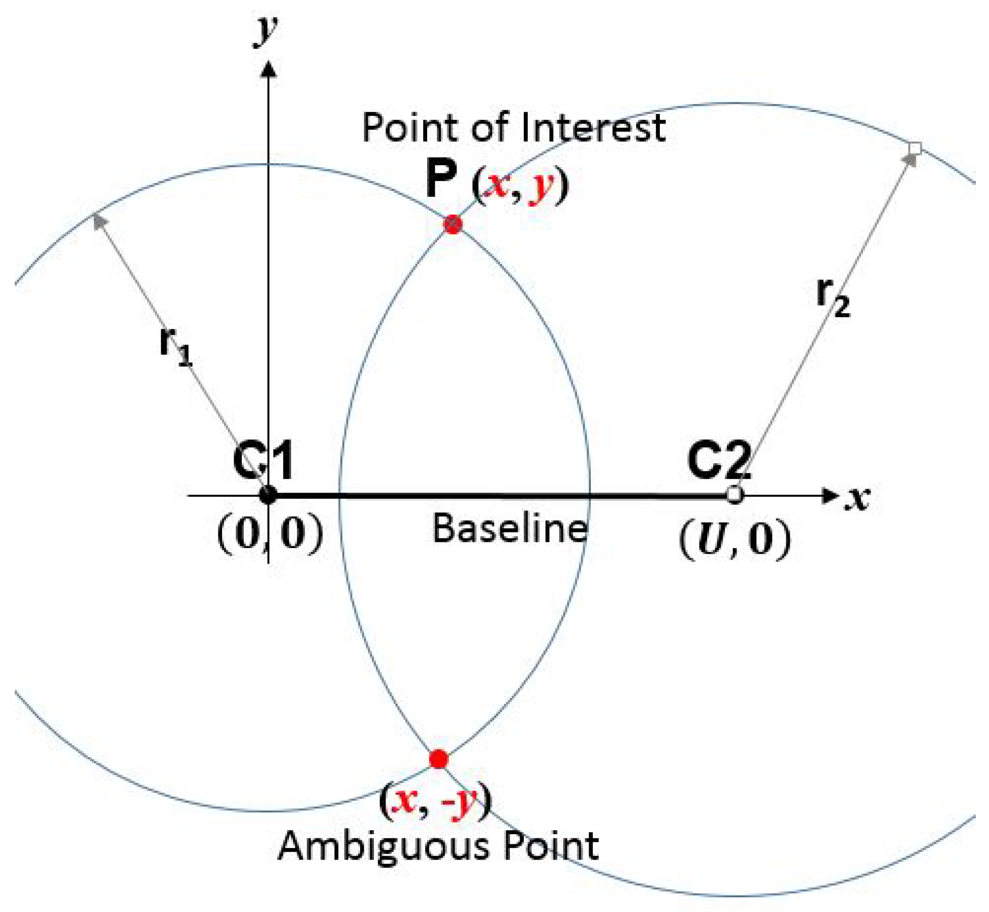
4.2. Triangulation
- Distance estimation:
- Position estimation:

4.3. Motion Sensors
4.4. Matching Data
4.4.1. Fingerprint
4.4.2. Point Cloud Matching
4.4.3. Image Matching
4.5. Optimization-Based Approches

4.5.1. Bundle Adjustment Based Methods
4.5.2. Graph Based Methods
4.6. Probability-Based Approches
- : is the belief on
- : is the observation model
- : is the motion model
4.6.1. Parametric Methods—Kalman Filter Family
- : is a matrix which represent the effect of the state on the parameters at time t
- : the covariance of the process noise
- : is a matrix that gives the effect pf the control input on the parameters
- : is the observation matrix that the state parameters to the measurement domain
- : is the co-variance matrix that describe the the correlation between parameters
- : is the motions noise
- : is the measurement noise
4.6.2. Non-Parametric Methods—Particle Filter Family
4.6.3. Localization with Filter-Based Methods
4.7. Cooperative Localization
- Vehicle-to-Vehicle (V2V): generate such a network between the vehicles where the information can be transmitted; this information (position, speed, orientation, etc.) can be used interchangeably between vehicles to perform principal tasks like avoiding collision, changing lines.
- Vehicle-to-Infrastructure (V2I): create communication between vehicles based on an intermediate infrastructure that is suitable to share information, from the node to any connected vehicles.
- Vehicle-to-people (V2P): most generally uses the interaction of vehicles and other road users like walking people, people using mobile devices or bicycles or wheelchairs, etc.
- Vehicle-to-Cloud (V2C): this is a technology that enables the vehicles to connect to the cloud-based on a cloud-based connected platform and via broadband cellular connectivity.
- Vehicle-to-X (V2X): Offers the possibility of connecting the vehicles with everything, which is a great idea because providing information from road users’ early gives enough time to execute, in a comfortable way, vehicles’ task and checking the prioritization so that to increase the safety.
4.8. Discussion, Challenges, and Future Directions
5. Security in Localization
| Name | Devices | Access | Attack Effect | Countermeasure |
|---|---|---|---|---|
| Malicious OBD devices | OBD | Physical |
|
|
| CAN access through OBD | CAN | Physical |
| |
| ECU access through CAN | ECU | Physical |
|
|
| ine LiDAR spoofing | LiDAR | Remote |
|
|
| LiDAR jamming | LiDAR | remote |
| |
| Radar spoofing | Radar | Remote |
|
|
| Radar jamming | Radar | Remote |
|
|
| GPS Spoofing | GPS | Remote |
|
|
| Camera blinding | Camera | Remote |
|
|
| Adversarial Images | Images | Remote |
|
|
| Falsified information | V2V &V2I | Remote |
|
|
6. Environmental Impact of Localization and Mapping Techniques in Self-Driving Vehicles
- Energy Consumption and Emission Reduction (air pollution): Self-driving vehicles require energy-intensive sensors, computing systems, and data centers for mapping, potentially increasing overall energy demand. Ref. [201] affirmed that a connection exists (mutual causation) between energy usage and CO2 emissions. Energy consumption influences CO2 emissions (in the near term), indicating that higher energy consumption might result in increased CO2 emissions, and conversely (in the extended period). The [202] paper mentioned that current autonomous electric vehicles, which are based on conventional propulsion systems, have limitations in terms of energy efficiency and power transmission. These limitations may hinder large-scale adoption in the future. To address this issue, a study was conducted to analyze the energy consumption and efficiency improvement of a medium-sized autonomous electric vehicle powered by wheel motors. The study involved the development of a numerical energy model, which was validated against real driving data and applied in a case study. The energy analysis focused on three driving conditions: flat road, uphill and downhill. This allowed the energy consumption to be examined and the potential for energy savings through the use of an in-wheel drive system. The analysis took into account factors such as regenerative braking, which allows energy to be recovered during deceleration. Energy consumption and regenerated energy were calculated based on vehicle dynamics and autonomous driving patterns specific to each driving cycle. A case study was conducted based on driving data from electric vehicles in West Los Angeles. In this chapter [203], the authors introduce a novel framework aimed at creating energy-efficient autonomous driving policies for shared roads. This innovative approach combines cognitive hierarchy theory and reinforcement learning to address the complexities of human driver behavior. Cognitive hierarchy theory is employed to model decision-making at various levels of rationality exhibited by human drivers. By comprehending human choices, autonomous vehicles (AVs) enhance their ability to predict and adjust to these behaviors, facilitating safe navigation on shared roads. The framework also integrates reinforcement learning, enabling AVs to continually learn from their environment and enhance their decision-making skills. This iterative learning process empowers AVs to adapt to changing road conditions, optimize energy usage, and ensure consistent safe performance. These vehicles grapple with the dual challenge of precise sub-centimeter and millisecond self-localization while maintaining energy efficiency. In this context, localization takes center stage. This paper [204] presents FEEL—an inventive indoor localization system that amalgamates three low-energy sensors: IMU (Inertial Measurement Unit), UWB (Ultra-Wideband), and radar. The authors elaborate on FEEL’s software and hardware architecture. The paper also introduces an Adaptive Sensing Algorithm (ASA) that optimizes energy usage by adapting sensing frequency according to environmental dynamics. By judiciously curtailing energy consumption, ASA achieves up to 20% energy savings with minimal impact on accuracy. Extensive performance evaluations across various scenarios underscore FEEL’s exceptional accuracy, with deviations of under 7cm from ground truth measurements, coupled with ultra-low latency of around 3ms. These findings underscore FEEL’s prowess in satisfying the stringent demands of AIV localization. The proposed control strategy in [205] considers energy consumption, mobility, and passenger comfort while enabling vehicles to pass signalized intersections without stops. The leader vehicle plans its trajectory using dynamic programming (DP), optimizing energy consumption and other factors. Following CAVs either use cooperative adaptive cruise control or plan their own trajectories based on intersection conditions. Simulation results demonstrate reduced energy consumption without compromising mobility.
- Sound and light pollution: Sound and luminous pollution are additional plausible environmental consequences associated with autonomous vehicle operation. The paper [206] aims to introduce the project “DICA-VE: Driving Information in a Connected and Autonomous Vehicle Environment: Impacts on Safety and Emissions”. It also proposes a comprehensive approach to evaluate driving behavior volatility and create alerts for mitigating road conflicts and noise emissions in a connected vehicle setting. While literature on autonomous driving often overlooks noise and light pollution, these issues carry significant consequences for ecosystems and communities. Quieter driving and reduced vehicle volume may alleviate noise pollution. Additionally, AVs driving in darker conditions could decrease artificial lighting. These considerations call for more attention [207].
- Smart cities: The idea of smart cities necessitates merging multiple technologies—immersive sensing, ubiquitous communication, robust computing, substantial storage, and high intelligence (SCCSI). These are pivotal for applications like public safety, autonomous driving, connected health, and smart living. Foreseeing the rise of advanced SCCSI-equipped autonomous vehicles in smart cities, [208] proposes a cost-efficient Vehicle as a Service (VaaS) model. In VaaS, SCCSI-capable vehicles act as mobile servers and communicators, delivering SCCSI services in smart cities. VaaS’s potential in smart cities is explored, including upgrades from traditional vehicular ad-hoc networks (VANETs). The VaaS architecture effectively renders SCCSI services, addressing architectural, service, incentive, security, and privacy aspects. The paper offers a sustainable approach using VaaS, shedding light on SCCSI integration in smart cities through autonomous vehicles for diverse applications. The research in [209] examines autonomous vehicles (AVs) as potential smart and sustainable urban transportation amidst rapid urbanization. Growing urban mobility needs necessitate sustainable solutions to counter adverse societal, economic, and environmental effects. Addressing privacy and cybersecurity risks is pivotal for AVs’ development in such cities. The study evaluates global government measures to manage these risks. Privacy and cybersecurity are vital factors in AVs’ smart and sustainable city integration. The authors review literature supporting AVs’ role in sustainable development. Governments enforce regulations or guidelines for privacy. Cybersecurity relies on existing regulations while partnering with private sector for improvements. Efforts by countries like the US, UK, China, and more, along with state-level actions, tackle AV-related risks. This study offers a comprehensive analysis of AVs’ privacy and cybersecurity implications in smart, sustainable cities. It underscores global governmental actions and their significance in ensuring safe AV deployment, providing insights crucial for future transport systems. The [210] paper introduces AutoDRIVE, a comprehensive research and education ecosystem for autonomous driving and smart city solutions. AutoDRIVE prototypes, simulates, and deploys cyber-physical solutions, offering both software and hardware-in-the-loop interfaces. It is modular, scalable, and supports various frameworks, accommodating single and multi-agent approaches. The paper showcases ecosystem capabilities through use-cases: autonomous parking, behavioral cloning, intersection traversal, and smart city management. AutoDRIVE validates hardware-software components in intelligent transportation systems. As an open-access platform, AutoDRIVE aids prototyping, simulation, and deployment in autonomous driving and smart cities. Its adaptability to diverse frameworks and expandability aligns with field trends. AutoDRIVE enhances research and education in autonomous driving effectively.
- Infrastructure optimization: The study in [211] explores integrating solar energy into mobility systems, particularly Solar-electric Autonomous Mobility-on-Demand (AMoD). Solar roofs on vehicles generate energy, impacting consumption. The aim is to optimize operations including passenger service, charging, and vehicle-to-grid (V2G) interactions. Authors model fleet management using graphs and a linear program. Applied to a Gold Coast case, results show 10–15% lower costs with solar-electric fleets vs. electric-only. Larger V2G batteries reduce expenses through energy trading and potential profits. This research highlights solar’s benefits in AMoD for cost savings and efficiency. The [212] paper optimizes the routing and charging infrastructure for Autonomous Mobility on Demand (AMoD) systems. With the advent of autonomy and electrical engineering, an AMoD system becomes possible. The authors propose a model for fleet and charging optimization. Using a mesoscopic approach, they create a time-invariant model that reflects routes and charging, taking into account vehicle charging. The road network is based on a digraph with isoenergetic arcs to achieve energy accuracy. The problem is a globally optimal mixed-integer linear program that is solved in less than 10 min, which is practical in the real world. Their approach is validated with case studies from taxis in New York City. Collaborative infrastructure optimization outperforms heuristics. Increasing the number of stations is not always beneficial.
- Software optimization: Software optimization is another important way to mitigate the environmental impact of self-driving vehicles. Authors of [213] confirmed that the energy consumption of edge processing reduces a car’s mileage with up to , making autonomous driving a difficult challenge for electric cars. Ref. [214] addresses the significant challenge of managing computational power consumption within autonomous vehicles, particularly for tasks involving artificial intelligence algorithms for sensing and perception. To overcome this challenge, the paper introduces an adaptive optimization method that dynamically distributes onboard computational resources across multiple vehicular subsystems. This allocation is determined by the specific context in which the vehicle operates, accounting for factors like autonomous driving scenarios. By tailoring resource allocation to the situation, the proposed approach aims to enhance overall performance and reduce energy usage compared to conventional computational setups. The authors conducted experiments to validate their approach, creating diverse autonomous driving scenarios. The outcomes highlighted that their adaptive optimization method effectively enhanced both performance and energy efficiency in autonomous vehicles. This research makes a significant contribution by addressing a key hurdle in autonomous vehicle development—optimizing computational resource allocation using real-time contextual information. Overall, the paper presents an innovative strategy to tackle the issue of high computational power consumption in autonomous vehicles. Through dynamic resource allocation based on context, it offers potential enhancements in performance and energy efficiency. The findings yield valuable insights for optimizing computational resource allocation in autonomous vehicles and provide guidance for future research in this area. Moreover, reliance on multiple sensors, resource-intensive deep-learning models, and powerful hardware for safe navigation comes with challenges. Certain sensing modalities can hinder perception and escalate energy usage. To counteract this, the authors of [215] introduce EcoFusion—an energy-conscious sensor fusion approach that adapts fusion based on context, curtailing energy consumption while preserving perception quality. The proposed approach surpasses existing methods, improving object detection by up to 9.5%, while reducing energy consumption by around 60% and achieving a 58% latency reduction on Nvidia Drive PX2 hardware. Beyond EcoFusion, the authors suggest context identification strategies and execute a joint optimization for energy efficiency and performance. Context-specific results validate the efficacy of their approach.
7. Conclusions
Author Contributions
Funding
Acknowledgments
Conflicts of Interest
References
- Road Traffic Injuries; World Health Organization: Geneva, Switzerland, 2021; Available online: https://www.who.int/news-room/fact-sheets/detail/road-traffic-injuries (accessed on 2 July 2021).
- Du, H.; Zhu, G.; Zheng, J. Why travelers trust and accept self-driving cars: An empirical study. Travel Behav. Soc. 2021, 22, 1–9. [Google Scholar] [CrossRef]
- Kopestinsky, A. 25 Astonishing Self-Driving Car Statistics for 2021. PolicyAdvice. 2021. Available online: https://policyadvice.net/insurance/insights/self-driving-car-statistics/ (accessed on 2 July 2021).
- Yurtsever, E.; Lambert, J.; Carballo, A.; Takeda, K. A Survey of Autonomous Driving: Common Practices and Emerging Technologies. IEEE Access 2020, 8, 58443–58469. [Google Scholar] [CrossRef]
- Jo, K.; Kim, J.; Kim, D.; Jang, C.; Sunwoo, M. Development of autonomous car-part i: Distributed system architecture and development process. IEEE Trans. Ind. Electron. 2014, 61, 7131–7140. [Google Scholar] [CrossRef]
- Blanco-Claraco, J.L. A Tutorial on SE(3) Transformation Parameterizations and On-Manifold Optimization. No. 3. 2021. Available online: https://arxiv.org/abs/2103.15980 (accessed on 2 July 2021).
- Sjafrie, H. Introduction to Self-Driving Vehicle Technology; Taylor Francis: Oxfordshire, UK, 2020. [Google Scholar]
- Piasco, N.; Sidibé, D.; Demonceaux, C.; Gouet-Brunet, V. A survey on Visual-Based Localization: On the benefit of heterogeneous data. Pattern Recognit. 2018, 74, 90–109. [Google Scholar] [CrossRef]
- Garcia-Fidalgo, E.; Ortiz, A. Vision-based topological mapping and localization methods: A survey. Rob. Auton. Syst. 2015, 64, 1–20. [Google Scholar] [CrossRef]
- Grigorescu, S.; Trasnea, B.; Cocias, T.; Macesanu, G. A survey of deep learning techniques for autonomous driving. J. Field Robot. 2020, 37, 362–386. [Google Scholar] [CrossRef]
- Wu, Y.; Wang, Y.; Zhang, S.; Ogai, H. Deep 3D Object Detection Networks Using LiDAR Data: A Review. IEEE Sens. J. 2021, 21, 1152–1171. [Google Scholar] [CrossRef]
- Liu, W.; Sun, J.; Li, W.; Hu, T.; Wang, P. Deep learning on point clouds and its application: A survey. Sensors 2019, 19, 4188. [Google Scholar] [CrossRef]
- Huang, B.; Zhao, J.; Liu, J. A Survey of Simultaneous Localization and Mapping with an Envision in 6G Wireless Networks. 2019, pp. 1–17. Available online: https://arxiv.org/abs/1909.05214 (accessed on 5 July 2021).
- Bresson, G.; Alsayed, Z.; Yu, L.; Glaser, S. Simultaneous Localization and Mapping: A Survey of Current Trends in Autonomous Driving. IEEE Trans. Intell. Veh. 2017, 2, 194–220. [Google Scholar] [CrossRef]
- Xia, L.; Cui, J.; Shen, R.; Xu, X.; Gao, Y.; Li, X. A survey of image semantics-based visual simultaneous localization and mapping: Application-oriented solutions to autonomous navigation of mobile robots. Int. J. Adv. Robot. Syst. 2020, 17, 1–17. [Google Scholar] [CrossRef]
- Durrant-Whyte, H.; Bailey, T. Simultaneous localization and mapping: Part I. IEEE Robot. Autom. Mag. 2006, 13, 99–110. [Google Scholar] [CrossRef]
- Günay, F.B.; Öztürk, E.; Çavdar, T.; Hanay, Y.S.; Khan, A.U.R. Vehicular Ad Hoc Network (VANET) Localization Techniques: A Survey; Springer Netherlands: Dordrecht, The Netherlands, 2021; Volume 28. [Google Scholar] [CrossRef]
- Kuutti, S.; Fallah, S.; Katsaros, K.; Dianati, M.; Mccullough, F.; Mouzakitis, A. A Survey of the State-of-the-Art Localization Techniques and Their Potentials for Autonomous Vehicle Applications. IEEE Internet Things J. 2018, 5, 829–846. [Google Scholar] [CrossRef]
- Badue, C.; Guidolini, R.; Carneiro, R.V.; Azevedo, P.; Cardoso, V.B.; Forechi, A.; Jesus, L.; Berriel, R.; Paixão, T.M.; Mutz, F.; et al. Self-driving cars: A survey. Expert Syst. Appl. 2021, 165, 113816. [Google Scholar] [CrossRef]
- Betz, J.; Zheng, H.; Liniger, A.; Rosolia, U.; Karle, P.; Behl, M.; Krovi, V.; Mangharam, R. Autonomous vehicles on the edge: A survey on autonomous vehicle racing. IEEE Open J. Intell. Transp. Syst. 2022, 3, 458–488. [Google Scholar] [CrossRef]
- Kim, D.; Chung, T.; Yi, K. Lane map building and localization for automated driving using 2D laser rangefinder. In Proceedings of the 2015 IEEE Intelligent Vehicles Symposium (IV), Seoul, Republic of Korea, 28 June–1 July 2015; pp. 680–685. [Google Scholar] [CrossRef]
- Im, J.; Im, S.; Jee, G.-I. Extended Line Map-Based Precise Vehicle Localization Using 3D LiDAR. Sensors 2018, 18, 3179. [Google Scholar] [CrossRef]
- Otsu, N. A Threshold Selection Method from Gray-Level Histograms. IEEE Trans. Syst. Man Cybern. 1979, 9, 62–66. [Google Scholar] [CrossRef]
- Zhang, Y.; Wang, J.; Wang, X.; Li, C.; Wang, L. A real-time curb detection and tracking method for UGVs by using a 3D-LiDAR sensor. In Proceedings of the 2015 IEEE Conference on Control Applications (CCA), Sydney, Australia, 21–23 September 2015; pp. 1020–1025. [Google Scholar] [CrossRef]
- Wang, L.; Zhang, Y.; Wang, J. Map-Based Localization Method for Autonomous Vehicles Using 3D-LiDAR. IFAC-PapersOnLine 2017, 50, 276–281. [Google Scholar] [CrossRef]
- Sefati, M.; Daum, M.; Sondermann, B.; Kreisköther, K.D.; Kampker, A. Improving vehicle localization using semantic and pole-like landmarks. In Proceedings of the 2017 IEEE Intelligent Vehicles Symposium (IV), Los Angeles, CA, USA, 11–14 June 2017; pp. 13–19. [Google Scholar] [CrossRef]
- Kummerle, J.; Sons, M.; Poggenhans, F.; Kuhner, T.; Lauer, M.; Stiller, C. Accurate and efficient self-localization on roads using basic geometric primitives. In Proceedings of the 2019 IEEE International Conference on Robotics and Automation (IEEE ICRA 2019), Montreal, QC, Canada, 20–24 May 2019; pp. 5965–5971. [Google Scholar] [CrossRef]
- Zhang, C.; Ang, M.H.; Rus, D. Robust LiDAR Localization for Autonomous Driving in Rain. In Proceedings of the 2018 IEEE/RSJ International Conference on Intelligent Robots and Systems, IROS 2018, Madrid, Spain, 1–5 October 2018; pp. 3409–3415. [Google Scholar] [CrossRef]
- Weng, L.; Yang, M.; Guo, L.; Wang, B.; Wang, C. Pole-Based Real-Time Localization for Autonomous Driving in Congested Urban Scenarios. In Proceedings of the 2018 IEEE International Conference on Real-time Computing and Robotics (RCAR), Kandima, Maldives, 1–5 August 2018; pp. 96–101. [Google Scholar] [CrossRef]
- Lu, F.; Chen, G.; Dong, J.; Yuan, X.; Gu, S.; Knoll, A. Pole-based Localization for Autonomous Vehicles in Urban Scenarios Using Local Grid Map-based Method. In Proceedings of the 5th International Conference on Advanced Robotics and Mechatronics, ICARM 2020, Shenzhen, China, 18–21 December 2020; pp. 640–645. [Google Scholar] [CrossRef]
- Schaefer, A.; Büscher, D.; Vertens, J.; Luft, L.; Burgard, W. Long-term vehicle localization in urban environments based on pole landmarks extracted from 3-D LiDAR scans. Rob. Auton. Syst. 2021, 136, 103709. [Google Scholar] [CrossRef]
- Gim, J.; Ahn, C.; Peng, H. Landmark Attribute Analysis for a High-Precision Landmark-based Local Positioning System. IEEE Access 2021, 9, 18061–18071. [Google Scholar] [CrossRef]
- Pang, S.; Kent, D.; Morris, D.; Radha, H. FLAME: Feature-Likelihood Based Mapping and Localization for Autonomous Vehicles. In Proceedings of the 2019 IEEE/RSJ International Conference on Intelligent Robots and Systems (IROS), Macau, China, 3–8 November 2019; pp. 5312–5319. [Google Scholar] [CrossRef]
- Yuming, H.; Yi, G.; Chengzhong, X.; Hui, K. Why semantics matters: A deep study on semantic particle-filtering localization in a LiDAR semantic pole-map. arXiv 2023, arXiv:2305.14038v1. [Google Scholar]
- Dong, H.; Chen, X.; Stachniss, C. Online Range Image-based Pole Extractor for Long-term LiDAR Localization in Urban Environments. In Proceedings of the 2021 European Conference on Mobile Robots (ECMR), Bonn, Germany, 31 August–3 September 2021. [Google Scholar] [CrossRef]
- Shipitko, O.; Kibalov, V.; Abramov, M. Linear Features Observation Model for Autonomous Vehicle Localization. In Proceedings of the 16th International Conference on Control, Automation, Robotics and Vision, ICARCV 2020, Shenzhen, China, 13–15 December 2020; pp. 1360–1365. [Google Scholar] [CrossRef]
- Shipitko, O.; Grigoryev, A. Ground vehicle localization with particle filter based on simulated road marking image. In Proceedings of the 32nd European Conference on Modelling and Simulation, Wilhelmshaven, Germany, 22–26 May 2018; pp. 341–347. [Google Scholar] [CrossRef]
- Shipitko, O.S.; Abramov, M.P.; Lukoyanov, A.S. Edge Detection Based Mobile Robot Indoor Localization. International Conference on Machine Vision. 2018. Available online: https://www.semanticscholar.org/paper/Edge-detection-based-mobile-robot-indoor-Shipitko-Abramov/51fd6f49579568417dd2a56e4c0348cb1bb91e78 (accessed on 17 July 2021).
- Wu, F.; Wei, H.; Wang, X. Correction of image radial distortion based on division model. Opt. Eng. 2017, 56, 013108. [Google Scholar] [CrossRef]
- Weng, L.; Gouet-Brunet, V.; Soheilian, B. Semantic signatures for large-scale visual localization. Multimed. Tools Appl. 2021, 80, 22347–22372. [Google Scholar] [CrossRef]
- Hekimoglu, A.; Schmidt, M.; Marcos-Ramiro, A. Monocular 3D Object Detection with LiDAR Guided Semi Supervised Active Learning. 2023. Available online: http://arxiv.org/abs/2307.08415v1 (accessed on 25 January 2024).
- Hungar, C.; Brakemeier, S.; Jürgens, S.; Köster, F. GRAIL: A Gradients-of-Intensities-based Local Descriptor for Map-based Localization Using LiDAR Sensors. In Proceedings of the IEEE Intelligent Transportation Systems Conference, ITSC 2019, Auckland, New Zealand, 27–30 October 2019; pp. 4398–4403. [Google Scholar] [CrossRef]
- Hungar, C.; Fricke, J.; Stefan, J.; Frank, K. Detection of Feature Areas for Map-based Localization Using LiDAR Descriptors. In Proceedings of the 16th Workshop on Posit. Navigat. and Communicat, Bremen, Germany, 23–24 October 2019. [Google Scholar] [CrossRef]
- Gu, B.; Liu, J.; Xiong, H.; Li, T.; Pan, Y. Ecpc-icp: A 6d vehicle pose estimation method by fusing the roadside LiDAR point cloud and road feature. Sensors 2021, 21, 3489. [Google Scholar] [CrossRef] [PubMed]
- Burt, A.; Disney, M.; Calders, K. Extracting individual trees from LiDAR point clouds using treeseg. Methods Ecol. Evol. 2019, 10, 438–445. [Google Scholar] [CrossRef]
- Charroud, A.; Yahyaouy, A.; Moutaouakil, K.E.; Onyekpe, U. Localisation and mapping of self-driving vehicles based on fuzzy K-means clustering: A non-semantic approach. In Proceedings of the 2022 International Conference on Intelligent Systems and Computer Vision (ISCV), Fez, Morocco, 8–19 May 2022. [Google Scholar]
- Charroud, A.; Moutaouakil, K.E.; Yahyaouy, A.; Onyekpe, U.; Palade, V.; Huda, M.N. Rapid localization and mapping method based on adaptive particle filters. Sensors 2022, 22, 9439. [Google Scholar] [CrossRef]
- Charroud, A.; Moutaouakil, K.E.; Yahyaouy, A. Fast and accurate localization and mapping method for self-driving vehicles based on a modified clustering particle filter. Multimed. Tools Appl. 2023, 82, 18435–18457. [Google Scholar] [CrossRef]
- Zou, Y.; Wang, X.; Zhang, T.; Liang, B.; Song, J.; Liu, H. BRoPH: An efficient and compact binary descriptor for 3D point clouds. Pattern Recognit. 2018, 76, 522–536. [Google Scholar] [CrossRef]
- Kiforenko, L.; Drost, B.; Tombari, F.; Krüger, N.; Buch, A.G. A performance evaluation of point pair features. Comput. Vis. Image Underst. 2016, 166, 66–80. [Google Scholar] [CrossRef]
- Logoglu, K.B.; Kalkan, S.; Temize, A.l. CoSPAIR: Colored Histograms of Spatial Concentric Surflet-Pairs for 3D object recognition. Rob. Auton. Syst. 2016, 75, 558–570. [Google Scholar] [CrossRef]
- Buch, A.G.; Kraft, D. Local point pair feature histogram for accurate 3D matching. In Proceedings of the 29th British Machine Vision Conference, BMVC 2018, Newcastle, UK, 3–6 September 2018; Available online: https://www.reconcell.eu/files/publications/Buch2018.pdf (accessed on 20 July 2021).
- Zhao, H.; Tang, M.; Ding, H. HoPPF: A novel local surface descriptor for 3D object recognition. Pattern Recognit. 2020, 103, 107272. [Google Scholar] [CrossRef]
- Wu, L.; Zhong, K.; Li, Z.; Zhou, M.; Hu, H.; Wang, C.; Shi, Y. Pptfh: Robust local descriptor based on point-pair transformation features for 3d surface matching. Sensors 2021, 21, 3229. [Google Scholar] [CrossRef]
- Yang, J.; Zhang, Q.; Xiao, Y.; Cao, Z. TOLDI: An effective and robust approach for 3D local shape description. Pattern Recognit. 2017, 65, 175–187. [Google Scholar] [CrossRef]
- Prakhya, S.M.; Lin, J.; Chandrasekhar, V.; Lin, W.; Liu, B. 3DHoPD: A Fast Low-Dimensional 3-D Descriptor. IEEE Robot. Autom. Lett. 2017, 2, 1472–1479. [Google Scholar] [CrossRef]
- Hu, Z.; Qianwen, T.; Zhang, F. Improved intelligent vehicle self-localization with integration of sparse visual map and high-speed pavement visual odometry. Proc. Inst. Mech. Eng. Part J. Automob. Eng. 2021, 235, 177–187. [Google Scholar] [CrossRef]
- Li, Y.; Hu, Z.; Cai, Y.; Wu, H.; Li, Z.; Sotelo, M.A. Visual Map-Based Localization for Intelligent Vehicles from Multi-View Site Matching. IEEE Trans. Intell. Transp. Syst. 2021, 22, 1068–1079. [Google Scholar] [CrossRef]
- Ge, G.; Zhang, Y.; Jiang, Q.; Wang, W. Visual features assisted robot localization in symmetrical environment using laser slam. Sensors 2021, 21, 1772. [Google Scholar] [CrossRef] [PubMed]
- DBow3. Source Code. 2017. Available online: https://github.com/rmsalinas/DBow3 (accessed on 26 July 2021).
- Holliday, A.; Dudek, G. Scale-invariant localization using quasi-semantic object landmarks. Auton. Robots 2021, 45, 407–420. [Google Scholar] [CrossRef]
- Wikipedia. Convolutional Neural Network. Available online: https://en.wikipedia.org/wiki/Convolutional_neural_network (accessed on 28 July 2021).
- Li, B.; Zhang, T.; Xia, T. Vehicle detection from 3D LiDAR using fully convolutional network. Robot. Sci. Syst. 2016, 12. [Google Scholar] [CrossRef]
- Minemura, K.; Liau, H.; Monrroy, A.; Kato, S. LMNet: Real-time multiclass object detection on CPU using 3D LiDAR. In Proceedings of the 2018 3rd Asia-Pacific Conference on Intelligent Robot Systems (ACIRS 2018), Singapore, 21–23 July 2018; pp. 28–34. [Google Scholar] [CrossRef]
- Zhou, Y.; Tuzel, O. VoxelNet: End-to-End Learning for Point Cloud Based 3D Object Detection. In Proceedings of the IEEE Conference on Computer Vision and Pattern Recognition (CVPR), Salt Lake City, UT, USA, 18–23 June 2018; pp. 4490–4499. [Google Scholar] [CrossRef]
- Beltrán, J.; Guindel, C.; Moreno, F.M.; Cruzado, D.; García, F.; Escalera, A.D.L. BirdNet: A 3D Object Detection Framework from LiDAR Information. In Proceedings of the 2018 21st International Conference on Intelligent Transportation Systems (ITSC), Maui, HI, USA, 4–7 November 2018; pp. 3517–3523. [Google Scholar] [CrossRef]
- Barrera, A.; Guindel, C.; Beltrán, J.; García, F. BirdNet+: End-to-End 3D Object Detection in LiDAR Bird’s Eye View. In Proceedings of the 2020 IEEE 23rd International Conference on Intelligent Transportation Systems (ITSC), Virtual, 20–23 September 2020. [Google Scholar] [CrossRef]
- Simon, M.; Milz, S.; Amende, K.; Gross, H.-M. Complex-YOLO: Real-time 3D Object Detection on Point Clouds. arXiv 2018, arXiv:1803.06199. Available online: https://arxiv.org/abs/1803.06199 (accessed on 27 July 2021).
- Ali, W.; Abdelkarim, S.; Zidan, M.; Zahran, M.; Sallab, A.E. YOLO3D: End-to-end real-time 3D oriented object bounding box detection from LiDAR point cloud. Lect. Notes Comput. Sci. 2019, 11131 LNCS, 716–728. [Google Scholar] [CrossRef]
- Te, G.; Zheng, A.; Hu, W.; Guo, Z. RGCNN: Regularized graph Cnn for point cloud segmentation. In Proceedings of the MM ’18 —26th ACM International Conference on Multimedia, Seoul, Republic of Korea, 22–26 October 2018; pp. 746–754. [Google Scholar] [CrossRef]
- Hua, B.S.; Tran, M.K.; Yeung, S.K. Pointwise Convolutional Neural Networks. In Proceedings of the IEEE Conference on Computer Vision and Pattern Recognition, Salt Lake City, UT, USA, 18–23 June 2018; pp. 984–993. [Google Scholar] [CrossRef]
- Li, Y.; Bu, R.; Sun, M.; Wu, W.; Di, X.; Chen, B. PointCNN: Convolution on X-transformed points. Adv. Neural Inf. Process. Syst. 2018, 2018, 820–830. [Google Scholar]
- Lan, S.; Yu, R.; Yu, G.; Davis, L.S. Modeling local geometric structure of 3D point clouds using geo-cnn. In Proceedings of the IEEE Conference on Computer Vision and Pattern Recognition, Long Beach, CA, USA, 16–20 June 2019; pp. 998–1008. [Google Scholar] [CrossRef]
- Wang, Y.; Sun, Y.; Liu, Z.; Sarma, S.E.; Bronstein, M.M.; Solomon, J.M. Dynamic graph Cnn for learning on point clouds. ACM Trans. Graph. 2019, 38, 1–12. [Google Scholar] [CrossRef]
- Xu, Y.; Fan, T.; Xu, M.; Zeng, L.; Qiao, Y. SpiderCNN: Deep learning on point sets with parameterized convolutional filters. Lect. Notes Comput. Sci. 2018, 11212 LNCS, 90–105. [Google Scholar] [CrossRef]
- Wang, D.Z.; Posner, I. Voting for voting in online point cloud object detection. In Robotics: Science and Systems; Sapienza University of Rome: Rome, Italy, 2015; Volume 11. [Google Scholar] [CrossRef]
- Qi, C.R.; Su, H.; Mo, K.; Guibas, L.J. PointNet: Deep learning on point sets for 3D classification and segmentation. In Proceedings of the—30th IEEE Conference on Computer Vision and Pattern Recognition (CVPR 2017), Honolulu, HI, USA, 21–26 July 2017; pp. 77–85. [Google Scholar] [CrossRef]
- Qi, C.R.; Yi, L.; Su, H.; Guibas, L.J. PointNet++: Deep hierarchical feature learning on point sets in a metric space. Adv. Neural Inf. Process. Syst. 2017, 2017, 5100–5109. [Google Scholar]
- Hao, D.; Xieyuanli, C.; Simo, S.; Cyrill, S. Online Pole Segmentation on Range Images for Long-term LiDAR Localization in Urban Environments. arXiv 2022, arXiv:2208.07364v1. [Google Scholar]
- Zhang, R.; Guo, Z.; Zhang, W.; Li, K.; Miao, X.; Cui, B.; Qiao, Y.; Gao, P.; Li, H. PointCLIP: Point Cloud Understanding by CLIP. [Abstract]. 2021. Available online: http://arxiv.org/abs/2112.02413v1 (accessed on 28 July 2021).
- Zhu, X.; Zhang, R.; He, B.; Zeng, Z.; Zhang, S.; Gao, P. PointCLIP V2: Adapting CLIP for Powerful 3D Open-world Learning. arXiv 2022, arXiv:2211.11682v1. [Google Scholar]
- Nichol, A.; Jun, H.; Dhariwal, P.; Mishkin, P.; Chen, M. Point-E: A System for Generating 3D Point Clouds from Complex Prompts. arXiv 2022, arXiv:2212.08751v1. [Google Scholar]
- Liu, V.; Vermeulen, J.; Fitzmaurice, G.; Matejka, J. 3DALL-E: Integrating Text-to-Image AI in 3D Design Workflows. In Proceedings of the Woodstock ’18: ACM Symposium on Neural Gaze Detection, Woodstock, NY, USA, 3–5 June 2018; ACM: New York, NY, USA, 2018; p. 20. [Google Scholar] [CrossRef]
- Kasten, Y.; Rahamim, O.; Chechik, G. Point-Cloud Completion with Pretrained Text-to-image Diffusion Models. arXiv 2023, arXiv:2306.10533v1. [Google Scholar]
- Chen, R.; Liu, Y.; Kong, L.; Zhu, X.; Ma, Y.; Li, Y.; Hou, Y.; Qiao, Y.; Wang, W. CLIP2Scene: Towards Label-efficient 3D Scene Understanding by CLIP. arXiv 2023, arXiv:2301.04926v2. [Google Scholar]
- Wong, K.; Gu, Y.; Kamijo, S. Mapping for autonomous driving: Opportunities and challenges. IEEE Intell. Transp. Syst. Mag. 2021, 13, 91–106. [Google Scholar] [CrossRef]
- Seif, H.G.; Hu, X. Autonomous driving in the iCity—HD maps as a key challenge of the automotive industry. Engineering 2016, 2, 159–162. [Google Scholar] [CrossRef]
- Gwon, G.P.; Hur, W.S.; Kim, S.W.; Seo, S.W. Generation of a precise and efficient lane-level road map for intelligent vehicle systems. IEEE Trans. Veh. Technol. 2017, 66, 4517–4533. [Google Scholar] [CrossRef]
- HD Map for Autonomous Vehicles Market, Markets-and-Markets. 2021. Available online: https://www.marketsandmarkets.com/Market-Reports/hd-map-autonomous-vehicle-market-141078517.html (accessed on 15 August 2021).
- Hausler, S.; Milford, M. P1-021: Map Creation, Monitoring and Maintenance for Automated Driving-Literature Review. 2021. Available online: https://imoveaustralia.com/wp-content/uploads/2021/01/P1%E2%80%90021-Map-creation-monitoring-and-maintenance-for-automated-driving.pdf (accessed on 7 September 2021).
- Herrtwich, R. The Evolution of the HERE HD Live Map at Daimler. 2018. Available online: https://360.here.com/the-evolution-of-the-hd-live-map (accessed on 7 September 2021).
- Chellapilla, K. ‘Rethinking Maps for Self-Driving’. Medium. 2018. Available online: https://medium.com/wovenplanetlevel5/https-medium-com-lyftlevel5-rethinking-maps-for-self-driving-a147c24758d6 (accessed on 6 September 2021).
- Vardhan, H. HD Maps: New Age Maps Powering Autonomous Vehicles. Geo Spatial Word. 2017. Available online: https://www.geospatialworld.net/article/hd-maps-autonomous-vehicles/ (accessed on 7 September 2021).
- Dahlström, T. How Accurate Are HD Maps for Autonomous Driving and ADAS Simulation? 2020. Available online: https://atlatec.de/en/blog/how-accurate-are-hd-maps-for-autonomous-driving-and-adas-simulation/ (accessed on 7 September 2021).
- Schreier, M. Environment representations for automated on-road vehicles. At-Automatisierungstechnik 2018, 66, 107–118. [Google Scholar] [CrossRef]
- Thrun, S. Probabilistic robotics. Commun. ACM 2002, 45, 52–57. [Google Scholar] [CrossRef]
- Elfring, J.; Torta, E.; Molengraft, R.v. Particle Filters: A Hands-On Tutorial. Sensors 2021, 21, 438. [Google Scholar] [CrossRef] [PubMed]
- Schumann, S. Why We’re Mapping Down to 20 cm Accuracy on Roads. HERE 360 blog. 2014. Available online: https://360.here.com/2014/02/12/why-were-mapping-down-to-20cm-accuracy-on-roads/ (accessed on 3 September 2021).
- Waymo. Building Maps for a Self-Driving Car. 2016. Available online: https://blog.waymo.com/2019/09/building-maps-for-self-driving-car.html (accessed on 11 September 2021).
- Tom- Tom, The Netherlands. HD Map—Highly Accurate Border-to-Border Model of the Road. 2017. Available online: http://download.tomtom.com/open/banners/HD-Map-Product-Info-Sheet-improved-1.pdf (accessed on 4 September 2021).
- Liu, R.; Wang, J.; Zhang, B. High Definition Map for Automated Driving: Overview and Analysis. J. Navig. 2020, 73, 324–341. [Google Scholar] [CrossRef]
- Sanborn. High Definition (HD) Maps for Autonomous Vehicles. 2019. Available online: https://www.sanborn.com/highly-automated-driving-maps-for-autonomous-vehicles/ (accessed on 4 September 2021).
- Ushr. Company Information. Available online: https://static1.squarespace.com/static/5a4d1c29017db266a358080\7/t/5ac25a1df950b77ed28e2d21/1522686495724/20180309_Snapsh\ot+Backgrounder_final.pdf (accessed on 4 September 2021).
- Self-Driving Safety Report NVIDIA, US. 2021. Available online: https://www.nvidia.com/en-us/self-driving-cars/safety-report/ (accessed on 4 September 2021).
- ZENRIN. Maps to the Future. 2020. Available online: http://www.zenrin-europe.com/ (accessed on 12 September 2021).
- NavInfo. Overview. 2021. Available online: https://navinfo.com/en/autonomousdriving (accessed on 13 September 2021).
- Korosec, K. This Startup Is Using Uber and Lyft Drivers to Bring Self-Driving Cars to Market Faster. The Verge, 2017. Available online: https://www.theverge.com/2017/7/19/16000272/lvl5-self-driving-car-tesla-map-LiDAR (accessed on 13 September 2021).
- Atlatec. High Definition Maps for Autonomous Driving and Simulation. 2021. Available online: https://atlatec.de/en/ (accessed on 13 September 2021).
- Zhang, H.; Chen, N.; Fan, G.; Yang, D. An improved scan matching algorithm in SLAM. In Proceedings of the 6th International Conference on Systems and Informatics (ICSAI 2019), Shanghai, China, 2–4 November 2019; pp. 160–164. [Google Scholar] [CrossRef]
- Jamil, F.; Iqbal, N.; Ahmad, S.; Kim, D.H. Toward accurate position estimation using learning to prediction algorithm in indoor navigation. Sensors 2020, 20, 4410. [Google Scholar] [CrossRef] [PubMed]
- Joram, N. Dead Reckoning—A Nature-Inspired Path Integration That Made Us Discover the New World. Medium. 2021. Available online: https://medium.com/geekculture/dead-reckoning-a-nature-inspired-path-integration-that-made-us-discover-the-new-world-ce67ee9d407d (accessed on 26 September 2021).
- Fuchs, C.; Aschenbruck, N.; Martini, P.; Wieneke, M. Indoor tracking for mission critical scenarios: A survey. Pervasive Mob. Comput. 2011, 7, 1–15. [Google Scholar] [CrossRef]
- Wikipedia. True-Range Multilateration. 2021. Available online: https://en.wikipedia.org/wiki/True-range_multilateration (accessed on 23 September 2021).
- Noureldin, A.; El-Shafie, A.; Bayoumi, M. GPS/INS integration utilizing dynamic neural networks for vehicular navigation. Inf. Fusion 2011, 12, 48–57. [Google Scholar] [CrossRef]
- Malleswaran, M.; Vaidehi, V.; Saravanaselvan, A.; Mohankumar, M. Performance analysis of various artificial intelligent neural networks for GPS/INS Integration. Appl. Artif. Intell. 2013, 27, 367–407. [Google Scholar] [CrossRef]
- Dai, H.f.; Bian, H.w.; Wang, R.y.; Ma, H. An INS/GNSS integrated navigation in GNSS denied environment using recurrent neural network. Def. Technol. 2020, 16, 334–340. [Google Scholar] [CrossRef]
- Onyekpe, U.; Palade, V.; Kanarachos, S.; Christopoulos, S.R.G. Learning Uncertainties in Wheel Odometry for Vehicular Localisation in GNSS Deprived Environments. In Proceedings of the 19th IEEE International Conference on Machine Learning and Applications (ICMLA 2020), Miami, FL, USA, 14–17 December 2020; pp. 741–746. [Google Scholar] [CrossRef]
- Onyekpe, U.; Palade, V.; Herath, A.; Kanarachos, S.; Fitzpatrick, M.E. WhONet: Wheel Odometry neural Network for vehicular localisation in GNSS-deprived environments. Eng. Appl. Artif. Intell. 2021, 105, 104421. [Google Scholar] [CrossRef]
- Harvey, S.; Lee, A. Introducing: The Fingerprint Base Map™ for Autonomous Vehicle Mapping and Localization. Medium. 2018. Available online: https://medium.com/@CivilMaps/introducing-the-fingerprint-base-map-for-autonomous-vehicle-mapping-and-localization-649dbd1e4810 (accessed on 26 September 2021).
- Besl, P.J.; McKay, N.D. A Method for Registration of 3-D Shapes. IEEE Trans. Pattern Anal. Mach. Intell. 1992, 14, 239–256. [Google Scholar] [CrossRef]
- Zhu, H.; Guo, B.; Zou, K.; Li, Y.; Yuen, K.V.; Mihaylova, L.; Leung, H. A review of point set registration: From pairwise registration to groupwise registration. Sensors 2019, 19, 1191. [Google Scholar] [CrossRef] [PubMed]
- Wang, F.; Zhao, Z. A survey of iterative closest point algorithm. In Proceedings of the 2017 Chinese Automation Congress (CAC), Jinan, China, 20–22 October 2017; Volume 2017, pp. 4395–4399. [Google Scholar] [CrossRef]
- Biber, P. The Normal Distributions Transform: A New Approach to Laser Scan Matching. IEEE Int. Conf. Intell. Robot. Syst. 2003, 3, 2743–2748. [Google Scholar] [CrossRef]
- Silver, D. NDT Matching, Medium. 2017. Available online: https://medium.com/self-driving-cars/ndt-matching-acff8e7e01cb (accessed on 27 September 2021).
- Shi, X.; Peng, J.; Li, J.; Yan, P.; Gong, H. The Iterative Closest Point Registration Algorithm Based on the Normal Distribution Transformation. Procedia Comput. Sci. 2019, 147, 181–190. [Google Scholar] [CrossRef]
- Wikipedia. Point Set Registration. Available online: https://en.wikipedia.org/wiki/Point_set_registration (accessed on 27 September 2021).
- Chui, H.; Rangarajan, A. A new point matching algorithm for non-rigid registration. Comput. Vis. Image Underst. 2003, 89, 114–141. [Google Scholar] [CrossRef]
- Jian, B.; Vemuri, B.C. Robust Point Set Registration Using Gaussian Mixture Models. IEEE Trans. Pattern Anal. Mach. Intell. 2011, 33, 1633–1645. [Google Scholar] [CrossRef]
- Yuan, W.; Eckart, B.; Kim, K.; Jampani, V.; Fox, D.; Kautz, J. DeepGMR: Learning Latent Gaussian Mixture Models for Registration. Lect. Notes Comput. Sci. 2020, 12350 LNCS, 733–750. [Google Scholar] [CrossRef]
- Deng, H.; Birdal, T.; Ilic, S. 3D local features for direct pairwise registration. In Proceedings of the IEEE Computer Society Conference on Computer Vision and Pattern Recognition, Long Beach, CA, USA, 16–17 June 2019; pp. 3239–3248. [Google Scholar] [CrossRef]
- Aoki, Y.; Goforth, H.; Srivatsan, R.A.; Lucey, S. Pointnetlk: Robust & efficient point cloud registration using pointnet. In Proceedings of the 2019 IEEE/CVF Conference on Computer Vision and Pattern Recognition (CVPR 2019), Long Beach, CA, USA, 15–20 June 2019; pp. 7156–7165. [Google Scholar] [CrossRef]
- Wang, Y.; Solomon, J. Deep closest point: Learning representations for point cloud registration. In Proceedings of the 2019 IEEE/CVF International Conference on Computer Vision (ICCV), Seoul, Republic of Korea, 27 October–2 November 2019; pp. 3522–3531. [Google Scholar] [CrossRef]
- Huang, X.; Mei, G.; Zhang, J.; Abbas, R. A Comprehensive Survey on Point Cloud Registration. 2021, pp. 1–17. Available online: https://arxiv.org/abs/2103.02690 (accessed on 10 August 2021).
- Woo, A.; Fidan, B.; Melek, W.W. Localization for Autonomous Driving. In Handbook of Position Location: Theory, Practice, and Advances; John Wiley: Hoboken, NJ, USA, 2019; pp. 1051–1087. [Google Scholar] [CrossRef]
- Jiang, Z.; Xu, Z.; Li, Y.; Min, H.; Zhou, J. Precise vehicle ego-localization using feature matching of pavement images. J. Intell. Connect. Veh. 2020, 3, 37–47. [Google Scholar] [CrossRef]
- Sivic, J.; Zisserman, A. Video google: A text retrieval approach to object matching in videos. In Proceedings of the Ninth IEEE International Conference on Computer Vision 2003, Nice, France, 13–16 October 2003; Volume 2, pp. 1470–1477. [Google Scholar] [CrossRef]
- Philbin, J.; Chum, O.; Isard, M.; Sivic, J.; Zisserman, A. Lost in quantization: Improving particular object retrieval in large scale image databases. In Proceedings of the 2008 IEEE Computer Society Conference on Computer Vision and Pattern Recognition (CVPR 2008), Anchorage, AK, USA, 24–26 June 2008. [Google Scholar] [CrossRef]
- Cao, S.; Snavely, N. Graph-based discriminative learning for location recognition. In Proceedings of the 2013 IEEE Conference on Computer Vision and Pattern Recognition, Portland, OR, USA, 23–28 June 2013; pp. 700–707. [Google Scholar] [CrossRef]
- Aubry, M.; Russell, B.C.; Sivic, J. Alignment via Discriminative Visual Elements. 2014. Available online: https://hal.inria.fr/hal-00863615v1/document (accessed on 11 August 2021).
- Lu, G.; Yan, Y.; Ren, L.; Song, J.; Sebe, N.; Kambhamettu, C. Localize Me Anywhere, Anytime: A Multi-task Point-Retrieval Approach. In Proceedings of the 2015 IEEE International Conference on Computer Vision (ICCV), Santiago, Chile, 7–13 December 2015; pp. 2434–2442. [Google Scholar] [CrossRef]
- Arth, C.; Pirchheim, C.; Ventura, J.; Schmalstieg, D.; Lepetit, V. Instant Outdoor Localization and SLAM Initialization from 2.5D Maps. IEEE Trans. Vis. Comput. Graph. 2015, 21, 1309–1318. [Google Scholar] [CrossRef]
- Poglitsch, C.; Arth, C.; Schmalstieg, D.; Ventura, J. [POSTER] A Particle Filter Approach to Outdoor Localization Using Image-Based Rendering. In Proceedings of the 2015 IEEE International Symposium on Mixed and Augmented Reality, Fukuoka, Japan, 29 September–3 October 2015; pp. 132–135. [Google Scholar] [CrossRef]
- Song, Y.; Chen, X.; Wang, X.; Zhang, Y.; Li, J. 6-DOF Image Localization From Massive Geo-Tagged Reference Images. IEEE Trans. Multimed. 2016, 18, 1542–1554. [Google Scholar] [CrossRef]
- Sattler, T.; Leibe, B.; Kobbelt, L. Efficient & Effective Prioritized Matching for Large-Scale Image-Based Localization. IEEE Trans. Pattern Anal. Mach. Intell. 2017, 39, 1744–1756. [Google Scholar] [CrossRef] [PubMed]
- Shotton, J.; Glocker, B.; Zach, C.; Izadi, S.; Criminisi, A.; Fitzgibbon, A. Scene Coordinate Regression Forests for Camera Relocalization in RGB-D Images. In Proceedings of the 2013 IEEE Conference on Computer Vision and Pattern Recognition (CVPR), Portland, OR, USA, 23–28 June 2013; pp. 2930–2937. [Google Scholar] [CrossRef]
- Kendall, A.; Grimes, M.; Cipolla, R. PoseNet: A Convolutional Network for Real-Time 6-DOF Camera Relocalization. In Proceedings of the 2015 IEEE International Conference on Computer Vision (ICCV), Santiago, Chile, 7–13 December 2015; pp. 2938–2946. [Google Scholar] [CrossRef]
- Ahmed, S.Z.; Saputra, V.B.; Verma, S.; Zhang, K.; Adiwahono, A.H. Sparse-3D LiDAR Outdoor Map-Based Autonomous Vehicle Localization. In Proceedings of the 2019 IEEE/RSJ International Conference on Intelligent Robots and Systems (IROS), Macau, China, 3–8 November 2019; pp. 1614–1619. [Google Scholar] [CrossRef]
- Zhang, J.; Ai, D.; Xiang, Y.; Wang, Y.; Chen, X.; Chang, X. Bag-of-words based loop-closure detection in visual SLAM. In Advanced Optical Imaging Technologies 2018; SPIE: Bellingham, WA, USA, 2018; Volume 1081618, p. 45. [Google Scholar] [CrossRef]
- Chen, Y.; Chen, Y.; Wang, G. Bundle Adjustment Revisited. 2019. Available online: https://arxiv.org/abs/1912.03858 (accessed on 15 August 2021).
- Li, J.; Pei, L.; Zou, D.; Xia, S.; Wu, Q.; Li, T.; Sun, Z.; Yu, W. Attention-SLAM: A Visual Monocular SLAM Learning from Human Gaze. IEEE Sens. J. 2021, 21, 6408–6420. [Google Scholar] [CrossRef]
- Burri, M.; Nikolic, J.; Gohl, P.; Schneider, T.; Rehder, J.; Omari, S.; Achtelik, M.W.; Siegwart, R. The EuRoC micro aerial vehicle datasets. Int. J. Rob. Res. 2016, 35, 1157–1163. [Google Scholar] [CrossRef]
- Mur-Artal, R.; Montiel, J.M.M.; Tardós, J.D. ORB-SLAM: A Versatile and Accurate Monocular SLAM System. IEEE Trans. Robot. 2015, 31, 1147–1163. [Google Scholar] [CrossRef]
- Liu, Z.; Zhang, F. BALM: Bundle Adjustment for LiDAR Mapping. IEEE Robot. Autom. Lett. 2021, 6, 3184–3191. [Google Scholar] [CrossRef]
- Zhang, J.; Singh, S. LOAM: LiDAR Odometry and Mapping in Real-time. Auton. Robots 2014, 41, 401–416. [Google Scholar] [CrossRef]
- Wang, K.; Ma, S.; Ren, F.; Lu, J. SBAS: Salient Bundle Adjustment for Visual SLAM. IEEE Trans. Instrum. Meas. 2021, 70, 1–11. [Google Scholar] [CrossRef]
- Lu, S.; Zhi, Y.; Zhang, S.; He, R.; Bao, Z. Semi-Direct Monocular SLAM with Three Levels of Parallel Optimizations. IEEE Access 2021, 9, 86801–86810. [Google Scholar] [CrossRef]
- Grisetti, G.; Kummerle, R.; Stachniss, C.; Burgard, W. A tutorial on graph-based SLAM. IEEE Intell. Transp. Syst. Mag. 2010, 2, 31–43. [Google Scholar] [CrossRef]
- Sualeh, M.; Kim, G.W. Simultaneous Localization and Mapping in the Epoch of Semantics: A Survey. Int. J. Control. Autom. Syst. 2019, 17, 729–742. [Google Scholar] [CrossRef]
- Stachniss, C. Graph-Based SLAM in 90 Minutes. BONN University, 2020. Available online: https://www.unravel.rwth-aachen.de/global/show_document.asp?id=aaaaaaaaabebgwr&do\wnload=1 (accessed on 5 October 2021).
- Mukherjee, S.; Kaess, M.; Martel, J.N.; Riviere, C.N. EyeSAM: Graph-based Localization and Mapping of Retinal Vasculature during Intraocular Microsurgery. Physiol. Behav. 2019, 176, 139–148. [Google Scholar] [CrossRef] [PubMed]
- Jung, S.; Choi, D.; Song, S.; Myung, H. Bridge inspection using unmanned aerial vehicle based on HG-SLAM: Hierarchical graph-based SLAM. Remote Sens. 2020, 12, 3022. [Google Scholar] [CrossRef]
- Jo, J.H.; Moon, C.B. Development of a Practical ICP Outlier Rejection Scheme for Graph-based SLAM Using a Laser Range Finder. Int. J. Precis. Eng. Manuf. 2019, 20, 1735–1745. [Google Scholar] [CrossRef]
- Akca, A.; Efe, M.Ö. Multiple Model Kalman and Particle Filters and Applications: A Survey. IFAC-PapersOnLine 2019, 52, 73–78. [Google Scholar] [CrossRef]
- Wadud, R.A.; Sun, W. DyOb-SLAM: Dynamic Object Tracking SLAM System. arXiv 2022, arXiv:2211.01941. [Google Scholar]
- Teed, Z.; Deng, J. DROID-SLAM: Deep Visual SLAM for Monocular, Stereo, and RGB-D Cameras. Adv. Neural Inf. Process. Syst. 2021, 34, 16558–16569. [Google Scholar]
- Li, Q.; Li, R.; Ji, K.; Dai, W. Kalman filter and its application. In Proceedings of the 8th International Conference on Intelligent Networks and Intelligent Systems (ICINIS 2015), Tianjin, China, 1–3 November 2015; pp. 74–77. [Google Scholar] [CrossRef]
- Chen, S.Y. Kalman filter for robot vision: A survey. IEEE Trans. Ind. Electron. 2012, 59, 4409–4420. [Google Scholar] [CrossRef]
- Li, W.; Wang, Z.; Yuan, Y.; Guo, L. Particle filtering with applications in networked systems: A survey. Complex Intell. Syst. 2016, 2, 293–315. [Google Scholar] [CrossRef]
- Gustafsson, F. Particle filter theory and practice with positioning applications. IEEE Aerosp. Electron. Syst. Mag. 2010, 25, 53–82. [Google Scholar] [CrossRef]
- Brossard, M.; Bonnabel, S.; Barrau, A. Invariant Kalman Filtering for Visual Inertial SLAM. In Proceedings of the 2018 21st International Conference on Information Fusion (FUSION), Cambridge, UK, 10–13 July 2018; pp. 2021–2028. [Google Scholar] [CrossRef]
- Bahraini, M.S. On the Efficiency of SLAM Using Adaptive Unscented Kalman Filter. Iran. J. Sci. Technol.-Trans. Mech. Eng. 2020, 44, 727–735. [Google Scholar] [CrossRef]
- Slowak, P.; Kaniewski, P. Stratified particle filter monocular SLAM. Remote Sens. 2021, 13, 3233. [Google Scholar] [CrossRef]
- Zhang, Q.; Li, Y.; Ma, T.; Cong, Z.; Zhang, W. Bathymetric Particle Filter SLAM with Graph-Based Trajectory Update Method. IEEE Access 2021, 9, 85464–85475. [Google Scholar] [CrossRef]
- Aghili, F. LiDAR SLAM for Autonomous Driving Vehicles. Int. J. Robot. Res. 2010, 29, 321–341. [Google Scholar] [CrossRef]
- Hyowon, K.; Karl, G.; Lennart, S.; Sunwoo, K.; Henk, W. PMBM-based SLAM Filters in 5G mmWave Vehicular Networks. arXiv 2022, arXiv:2205.02502v1. [Google Scholar]
- Chiu, C.-Y. SLAM Backends with Objects in Motion: A Unifying Framework and Tutorial. In Proceedings of the 2023 American Control Conference (ACC), San Diego, CA, USA, 31 May–2 June 2023; pp. 1635–1642. [Google Scholar] [CrossRef]
- Zeadally, S.; Guerrero, J.; Contreras, J. A tutorial survey on vehicle-to-vehicle communications. Telecommun. Syst. 2020, 73, 469–489. [Google Scholar] [CrossRef]
- Chehri, A.; Quadar, N.; Saadane, R. Survey on localization methods for autonomous vehicles in smart cities. In Proceedings of the SCA ’19: 4th International Conference on Smart City Applications, Casablanca, Morocco, 2–4 October 2019. [Google Scholar] [CrossRef]
- Aoki, S.; Rajkumar, R.R. A-DRIVE: Autonomous Deadlock Detection and Recovery at Road Intersections for Connected and Automated Vehicles. Available online: http://arxiv.org/abs/2204.04910v1 (accessed on 11 April 2022).
- Piperigkos, N.; Lalos, A.S.; Berberidis, K. Graph Laplacian Diffusion Localization of Connected and Automated Vehicles. IEEE Trans. Intell. Transp. Syst. 2022, 23, 12176–12190. [Google Scholar] [CrossRef]
- Typaldos, P.; Papageorgiou, M.; Papamichail, I. Optimization-based path-planning for connected and non-connected Automated Vehicles. Transp. Res. Part Emerg. Technol. 2022, 134, 103487. [Google Scholar] [CrossRef]
- Katriniok, A.; Rosarius, B.; Mähönen, P. Fully Distributed Model Predictive Control of Connected Automated Vehicles in Intersections: Theory and Vehicle Experiments. IEEE Trans. Intell. Transp. Syst. 2022, 23, 18288–18300. [Google Scholar] [CrossRef]
- Ploeg, C.v.; Smit, R.; Siagkris-Lekkos, A.; Benders, F.; Silvas, E. Anomaly Detection from Cyber Threats via Infrastructure to Automated Vehicle. In Proceedings of the 2021 European Control Conference (ECC), Delft, The Netherlands, 29 June–2 July 2021; pp. 1788–1794. [Google Scholar] [CrossRef]
- Soatti, G.; Nicoli, M.; Garcia, N.; Denis, B.; Raulefs, R.; Wymeersch, H. Implicit cooperative positioning in vehicular networks. IEEE Trans. Intell. Transp. Syst. 2018, 19, 3964–3980. [Google Scholar] [CrossRef]
- Ghaleb, F.A.; Zainal, A.; Rassam, M.A.; Abraham, A. Improved vehicle positioning algorithm using enhanced innovation-based adaptive Kalman filter. Pervasive Mob. Comput. 2017, 40, 139–155. [Google Scholar] [CrossRef]
- Shao, Z.; Li, W.; Wu, Y.; Shen, L. Multi-layer and multi-dimensional information based cooperative vehicle localization in highway scenarios. In Proceedings of the 2010 IEEE 12th International Conference on Communication Technology, Nanjing, China, 11–14 November 2010; pp. 567–571. [Google Scholar] [CrossRef]
- Hoang, G.M.; Denis, B.; Harri, J.; Slock, D.T.M. Robust data fusion for cooperative vehicular localization in tunnels. In Proceedings of the 2017 IEEE Intelligent Vehicles Symposium, Los Angeles, CA, USA, 11–14 June 2017; pp. 1372–1377. [Google Scholar] [CrossRef]
- Chen, H.; Luo, R.; Feng, Y. Improving Autonomous Vehicle Mapping and Navigation in Work Zones Using Crowdsourcing Vehicle Trajectories. 2022. Available online: http://arxiv.org/abs/2301.09194v1 (accessed on 15 August 2021).
- Klupacs, J.; Gostar, A.K.; Bab-Hadiashar, A.; Palmer, J.; Hoseinnezhad, R. Distributed Complementary Fusion for Connected Vehicles. In Proceedings of the 2022 11th International Conference on Control, Automation and Information Sciences (ICCAIS), Hanoi, Vietnam, 21–24 November 2022; pp. 316–321. [Google Scholar] [CrossRef]
- Pham, M.; Xiong, K. A survey on security attacks and defense techniques for connected and autonomous vehicles. Comput. Secur. 2021, 109, 1–24. [Google Scholar] [CrossRef]
- Kukkala, V.; Thiruloga, S.V.; Pasricha, S. Roadmap for Cybersecurity in Autonomous Vehicles. IEEE Consum. Electron. Mag. 2022, 11, 13–23. [Google Scholar] [CrossRef]
- Yang, T.; Lv, C. Secure Estimation and Attack Isolation for Connected and Automated Driving in the Presence of Malicious Vehicles. IEEE Trans. Veh. Technol. 2021, 70, 8519–8528. [Google Scholar] [CrossRef]
- Ahn, N.; Lee, D.H. Vehicle Communication using Hash Chain-based Secure Cluster. arXiv 2019, arXiv:1912.12392. [Google Scholar]
- Ahn, N.Y.; Lee, D.H. Physical Layer Security of Autonomous Driving: Secure Vehicle-to-Vehicle Communication in A Security Cluster. arXiv 2019, arXiv:1912.06527. [Google Scholar]
- Halabi, J.; Artail, H. A Lightweight Synchronous Cryptographic Hash Chain Solution to Securing the Vehicle CAN bus. In Proceedings of the 2018 IEEE International Multidisciplinary Conference on Engineering Technology (IMCET), Beirut, Lebanon, 14–16 November 2018; pp. 1–6. [Google Scholar] [CrossRef]
- Cho, K.T.; Shin, K.G. Fingerprinting electronic control units for vehicle intrusion detection. In Proceedings of the 25th USENIX Security Symposium, Austin, TX, USA, 10–12 August 2016; pp. 911–927. Available online: https://www.usenix.org/system/files/conference/usenixsecurity16/sec16papercho.pdf (accessed on 11 August 2021).
- Regulus Cyber LTD. Tesla Model 3 Spoofed off the Highway–Regulus Navigation System Hack Causes Car to Turn on Its Own. Regulu. 2019. Available online: https://www.regulus.com/blog/tesla-model-3-spoofed-off-the-highway-regulus-navigationsystem-hack-causes-car-to-turn-on-its-own#:~:text=Actual%20control%20of%20the%20car,while%20driving\%20with%20NOA%20engaged (accessed on 20 October 2021).
- Stottelaar, B.G. Practical Cyber-Attacks on Autonomous Vehicles. 2015. Available online: http://essay.utwente.nl/66766/ (accessed on 11 August 2021).
- Shoukry, Y.; Martin, P.; Yona, Y.; Diggavi, S.; Srivastava, M. PyCRA: Physical challenge-response authentication for active sensors under spoofing attacks. In Proceedings of the CCS’15: The 22nd ACM Conference on Computer and Communications Security, Denver, CO, USA, 12–16 October 2015; pp. 1004–1015. [Google Scholar] [CrossRef]
- Petit, J.; Stottelaar, B.; Feiri, M.; Kargl, F. Remote Attacks on Automated Vehicles Sensors: Experiments on Camera and LiDAR. Blackhat.com. 2015, pp. 1–13. Available online: https://www.blackhat.com/docs/eu-15/materials/eu-15-Petit-Self-Driving-And-Connected-Cars-Fooling-Sensors-And-Tracking-Drivers-wp1.pdf (accessed on 11 August 2021).
- Chontanawat, J. Relationship between energy consumption, CO2 emission and economic growth in ASEAN: Cointegration and Causality Model. Energy Rep. 2020, 6, 660–665. [Google Scholar] [CrossRef]
- Shen, K.; Ke, X.; Yang, F.; Wang, W.; Zhang, C.; Yuan, C. Numerical Energy Analysis of In-wheel Motor Driven Autonomous Electric Vehicles. IEEE Trans. Transp. Electrif. 2023, 9, 3662–3676. [Google Scholar] [CrossRef]
- Li, H.; Li, N.; Kolmanovsky, I.; Girard, A. Energy-Efficient Autonomous Driving Using Cognitive Driver Behavioral Models and Reinforcement Learning. In AI-Enabled Technologies for Autonomous and Connected Vehicles; Murphey, Y.L., Kolmanovsky, I., Watta, P., Eds.; Lecture Notes in Intelligent Transportation and Infrastructure; Springer: Cham, Switzerland, 2023. [Google Scholar] [CrossRef]
- Gokhale, V.; Barrera, G.M.; Prasad, R.V. FEEL: Fast, Energy-Efficient Localization for Autonomous Indoor Vehicles. In Proceedings of the ICC 2021—IEEE International Conference on Communications, Montreal, QC, Canada, 14–18 June 2021; pp. 1–6. [Google Scholar] [CrossRef]
- Zhen, H.; Mosharafian, S.; Yang, J.J.; Velni, J.M. Eco-driving trajectory planning of a heterogeneous platoon in urban environments. IFAC-PapersOnLine 2022, 55, 161–166. [Google Scholar] [CrossRef]
- Coelho, M.C.; Guarnaccia, C. Driving information in a transition to a connected and autonomous vehicle environment: Impacts on pollutants, noise and safety. Transp. Res. Procedia 2020, 45, 740–746. [Google Scholar] [CrossRef]
- Silva, Ó.; Cordera, R.; González-González, E.; Nogués, S. Environmental impacts of autonomous vehicles: A review of the scientific literature. Sci. Total Environ. 2022, 830, 154615. [Google Scholar] [CrossRef]
- Chen, X.; Deng, Y.; Ding, H.; Qu, G.; Zhang, H.; Li, P.; Fang, Y. Vehicle as a Service (VaaS): Leverage Vehicles to Build Service Networks and Capabilities for Smart Cities. arXiv 2023, arXiv:2304.11397. [Google Scholar]
- Lim, H.; Taeihagh, A. Autonomous Vehicles for Smart and Sustainable Cities: An In-Depth Exploration of Privacy and Cybersecurity Implications. Energies 2018, 11, 1062. [Google Scholar] [CrossRef]
- Samak, T.; Samak, C.; Kandhasamy, S.; Krovi, V.; Xie, M. AutoDRIVE: A Comprehensive, Flexible and Integrated Digital Twin Ecosystem for Autonomous Driving Research & Education. Robotics 2023, 12, 77. [Google Scholar] [CrossRef]
- Paparella, F.; Hofman, T.; Salazar, M. Cost-optimal Fleet Management Strategies for Solar-electric Autonomous Mobility-on-Demand Systems. arXiv 2023, arXiv:2305.18816. [Google Scholar]
- Luke, J.; Salazar, M.; Rajagopal, R.; Pavone, M. Joint Optimization of Autonomous Electric Vehicle Fleet Operations and Charging Station Siting. In Proceedings of the 2021 IEEE International Intelligent Transportation Systems Conference (ITSC), Indianapolis, IN, USA, 19–22 September 2021; pp. 3340–3347. [Google Scholar] [CrossRef]
- Teraki. Autonomous Cars’ Big Problem: The Energy Consumption of Edge Processing Reduces a Car’s Mileage with up to 30%. 15 May 2019. Available online: https://medium.com/@teraki/energy-consumption-required-by-edge-computing-reduces-a-autonomous-cars-mileage-with-up-to-30-46b6764ea1b7 (accessed on 10 October 2023).
- Jambotkar, S.; Guo, L.; Jia, Y. Adaptive Optimization of Autonomous Vehicle Computational Resources for Performance and Energy Improvement. In Proceedings of the 2021 IEEE/RSJ International Conference on Intelligent Robots and Systems (IROS), Prague, Czech Republic, 27 September–1 October 2021; pp. 7594–7600. [Google Scholar] [CrossRef]
- Malawade, A.V.; Mortlock, T.; Faruque, M.A. EcoFusion: Energy-aware adaptive sensor fusion for efficient autonomous vehicle perception. In Proceedings of the 59th ACM/IEEE Design Automation Conference (DAC ’22), San Francisco, CA, USA, 10–14 July 2022; pp. 481–486. [Google Scholar] [CrossRef]
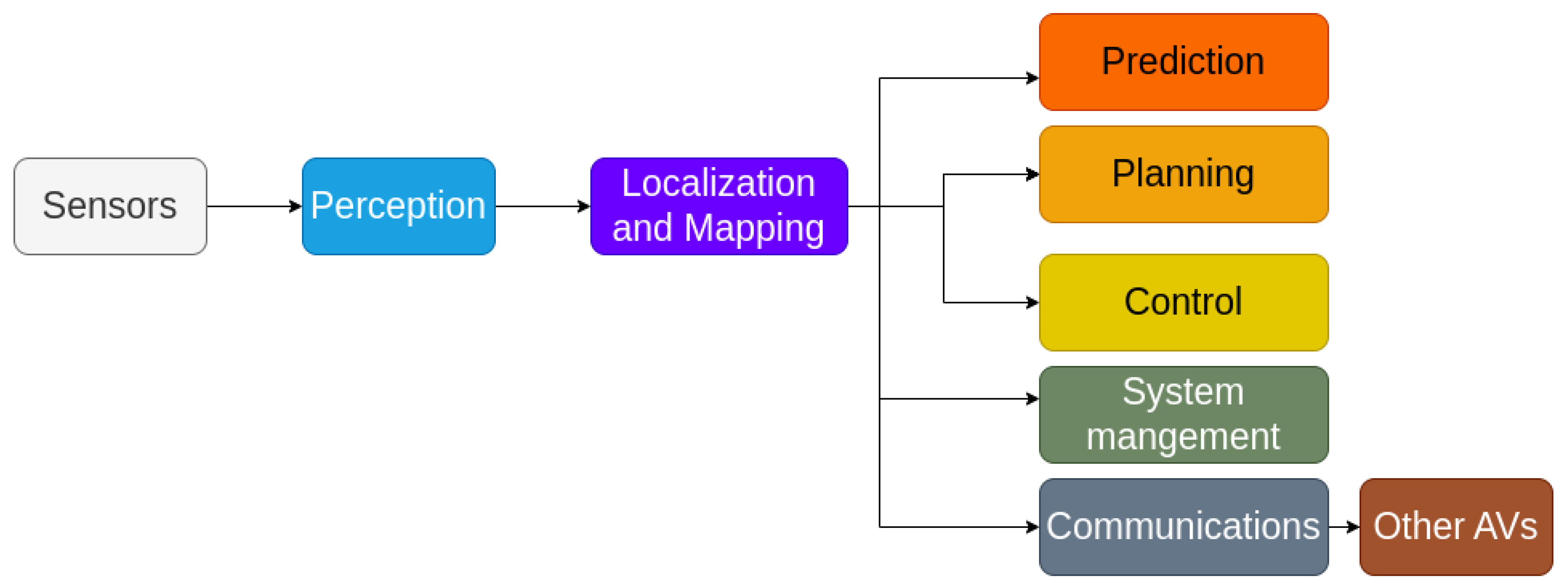


| Survey | Sensors | Features Extraction | Mapping | Ego-Localization | Co-Localization | SLAM | Security Autonomous | Environmental Impact | Challenges and Future Directions |
|---|---|---|---|---|---|---|---|---|---|
| [4] | GPS/INS Cameras LiDAR | Middle | Middle | Middle | No | Middle | Limited | No | Limited |
| [8] | Cameras | Extensive | Limited | Extensive | No | Middle | No | No | Middle |
| [9] | Cameras | Extensive | Limited | Extensive | No | Middle | No | No | Middle |
| [10] | Cameras LiDAR | Limited | Limited | Extensive | No | Limited | No | No | Extensive |
| [11] | LiDAR | Extensive | No | No | No | No | No | No | Extensive |
| [12] | LiDAR | Extensive | No | No | No | No | No | No | Extensive |
| [13] | Cameras LiDAR | Limited | Extensive | Extensive | No | Extensive | No | No | Extensive |
| [14] | Cameras LiDAR | Limited | Extensive | Extensive | No | Extensive | No | No | Extensive |
| [15] | Cameras | Limited | Extensive | Extensive | No | Extensive | No | No | Extensive |
| [16] | Cameras LiDAR | Limited | Extensive | Extensive | No | Extensive | No | No | Extensive |
| [17] | Cameras LiDAR | Limited | Extensive | Extensive | Extensive | Extensive | No | No | Extensive |
| [18] | All | No | Middle | Extensive | Extensive | Limited | Limited | No | Limited |
| [19] | Cameras LiDAR | Extensive | Extensive | Extensive | No | Limited | No | No | Limited |
| [20] | GPS/INS Cameras LiDAR | Limited | Limited | Extensive | No | Limited | No | No | Extensive |
| Ours | GPS/INS Cameras LiDAR | Extensive | Extensive | Extensive | Extensive | Extensive | Extensive | Extensive | Extensive |
| Approach | Sensors | Score | Main Challenges |
|---|---|---|---|
| Dead Reckoning | GPS INS Wheel odometry | Low | Prone to error in case drifting |
| Triangulation | GNSS | High | Limited in some environment senarios |
| Motion tracking | LiDAR Cameras | Passable | High cost of time and energy A few objects in the environment mislead the matching process. |
| Optimization | LiDAR Cameras | High | High computational time to solve the matrix calculation |
| Probability | LiDAR Cameras | High | Problem of initialization |
| Cooperative localization | Vehicle connectivity | High | Limitation if there is a long distance between vehicles |
Disclaimer/Publisher’s Note: The statements, opinions and data contained in all publications are solely those of the individual author(s) and contributor(s) and not of MDPI and/or the editor(s). MDPI and/or the editor(s) disclaim responsibility for any injury to people or property resulting from any ideas, methods, instructions or products referred to in the content. |
© 2024 by the authors. Licensee MDPI, Basel, Switzerland. This article is an open access article distributed under the terms and conditions of the Creative Commons Attribution (CC BY) license (https://creativecommons.org/licenses/by/4.0/).
Share and Cite
Charroud, A.; El Moutaouakil, K.; Palade, V.; Yahyaouy, A.; Onyekpe, U.; Eyo, E.U. Localization and Mapping for Self-Driving Vehicles: A Survey. Machines 2024, 12, 118. https://doi.org/10.3390/machines12020118
Charroud A, El Moutaouakil K, Palade V, Yahyaouy A, Onyekpe U, Eyo EU. Localization and Mapping for Self-Driving Vehicles: A Survey. Machines. 2024; 12(2):118. https://doi.org/10.3390/machines12020118
Chicago/Turabian StyleCharroud, Anas, Karim El Moutaouakil, Vasile Palade, Ali Yahyaouy, Uche Onyekpe, and Eyo U. Eyo. 2024. "Localization and Mapping for Self-Driving Vehicles: A Survey" Machines 12, no. 2: 118. https://doi.org/10.3390/machines12020118
APA StyleCharroud, A., El Moutaouakil, K., Palade, V., Yahyaouy, A., Onyekpe, U., & Eyo, E. U. (2024). Localization and Mapping for Self-Driving Vehicles: A Survey. Machines, 12(2), 118. https://doi.org/10.3390/machines12020118