
An Adapted NURBS Interpolator with a Switched Optimized Method of Feed-Rate Scheduling
College of Engineering, Harbin University, Harbin 150000, China
Machines 2024, 12(3), 186; https://doi.org/10.3390/machines12030186
Submission received: 6 February 2024
/
Revised: 29 February 2024
/
Accepted: 11 March 2024
/
Published: 13 March 2024
(This article belongs to the Section Advanced Manufacturing)
Abstract
:With the increasing demand for processing precision in the manufacturing industry, feed-rate scheduling is a crucial component in achieving the processing quality of complex surfaces. A smooth feed-rate profile not only guarantees machining quality but also improves machining efficiency. Although the typical offline feed-rate scheduling method possesses good processing efficiency, it may not provide an optimal solution due to the NP-hard problem caused by the feed-rate scheduling of continuous curve segments, which easily results in excess kinetic limitations and feed-rate fluctuations in a real-time interpolation. Instead, the FIR (Finite Impulse Response) method is widely used to realize interpolation in real-time processing. However, the FIR method will filter out a large number of high-frequency signals, leading to a low-processing efficiency. Further, greater acceleration or deceleration is required to ensure the interpolation passes through the segment end at a predefined feed rate and the deceleration in the feed rate profile appears earlier, which allows the interpolation to easily exceed the kinetic limitation. At present, a simple offline or online method cannot realize the global optimization of the feed-rate profile and guarantee the machining efficiency. Moreover, the current feed-rate scheduling that considers both offline and online methods does not consider the situation that the call of offline data and online prediction data will lead to a decrease in the real-time performance of the CNC system. Further, real-time feed-rate scheduling data tend to dominate the whole interpolation process, thus reducing the effect of the offline feed-rate scheduling data. Hence, based on the tool path with C3 continuity (Cubic Continuously Differentiable), this paper first presents a basic interpolation unit relevant to the S-type interpolation feed-rate profile. Then, an offline local smooth strategy is proposed to smooth the feed-rate profile and reduce the exceeding of kinetic limitations and feed-rate fluctuations caused by frequent acceleration and deceleration. Further, a global online smoothing strategy based on the data generated by offline pre-interpolation is presented. What is more, FIR login and logout conditions are proposed to further smooth the feed-rate profile and improve the real-time performance and machining efficiency. The case study validates that the proposed method performs better in kinetic results compared with the typical offline and FIR methods in both the simulation experiment and actual machining experiments. Especially, in actual processing experiments, the proposed method obtains a 28% reduction in contour errors. Further, the proposed method compared with the FIR method obtains a 15% increase in machining efficiency but only a 4% decrease compared with the typical offline method.
1. Introduction
With the continuous development of the manufacturing industry, the processing efficiency and quality of complex surface parts are increasingly required by end users. Traditional linear or circular interpolation is not smooth enough, which easily leads to frequent acceleration and deceleration and further affects the processing quality. Therefore, the parameter interpolation technology of the nonuniform rational B-spline (NURBS) interpolation [1,2] has become the main method to obtain a smoother tool path and feed-rate profile. As feed-rate scheduling is one of the key parts of parameter interpolation [3], a smoother feed-rate profile cannot only improve processing efficiency and ensure processing accuracy but also extend the life of the machine tool. Therefore, a large number of studies have focused on this issue to obtain a smoother feed-rate profile. At present, there are two methods of feed-rate scheduling to obtain a smoother feed-rate profile: offline feed-rate scheduling and online feed-rate scheduling.
Offline feed-rate scheduling. ZHANG [4] establishes a generalized representation for the nonlinear feed-rate scheduling model, with static and dynamic feed-rate constraints, through a numerical convex transformation. Beudaert [5] presented a VPO (Velocity Profile Optimization) method to obtain an optimized feed-rate profile that makes the best use of the kinematical characteristics of the machine tool. ZHANG [6] proposed an analytical one-step corner-smoothing method based on feed-rate blending to tackle the bottlenecks of linear interpolation and two-step geometry-based corner-smoothing methods in five-axis machining. HUANG [7] presents an analytical continuous-smoothing method for the five-axis toolpath by simultaneously scheduling the tool position and tool-orientation trajectories. Then, a time-synchronization strategy is proposed to realize the feed-rate scheduling. LIU [8] proposed a feed-rate planning module to obtain the restricted feed rate at the sharp corners of the NURBS curve, as well as an acc–jerk continuous module to achieve continuous acceleration and jerk. Mizoue [9] proposed a strategy for error compensation to optimize the feed-profile schedule for a single-step input. XU [10] adopted an S-shape acceleration/deceleration control to adjust the jerk, which can avoid the problem of feeding-speed overrun. At the same time, an interpolation parameter-calculation method is proposed to solve the problem of velocity error in the interpolation point-parameter calculation. HAN [11] introduced a feed-rate scheduling method for smooth time-dependent processing beams, which optimizes the feed rate within the dynamic constraints of the machine tool by establishing acceptable path spacing and feed ranges. Erkorkmaz [12] introduces a new optimization algorithm that combines linear programming and a windowing algorithm for optimizing the feed rates of spline tool paths. The algorithm has linear computational complexity and can process long tool paths in parallel. The offline feed-rate method is usually used to optimize kinetic profiles before real-time interpolation, which can obtain a reasonable machining efficiency. Especially for high-curvature segments, it can solve the singular points in the feed-rate profile that cause abnormal kinetic parameters and feed-rate fluctuations. However, when it comes to the transition of continuous high-curvature segments, the offline method relies too much on specific feed-rate scheduling models. If the model is not sufficient to complete the feed-rate scheduling tasks or there is no optimal solution in the multi-objective optimization problems [13] caused by the transition of continuous high-curvature segments, it may lead to large errors as the kinetic parameters do not comply with the kinetic constraints. Moreover, offline methods require significant effort in model accuracy and solving multi-objective optimization problems. Although there are many solutions for multi-objective optimization problems [14,15], it is still difficult to apply them to the actual processing due to the complexity of interpolation conditions and the high consumption of system resources. Therefore, it remains a challenge to increase the universality of the offline feed-rate scheduling models and eliminate the influence caused by the absence of optimal solutions in multi-objective optimization, which is one of the focuses of this work.
Online feed-rate scheduling. FAN [16] introduced a jerk-smooth feed-rate model to perform time-optimal feed-rate scheduling and then applied it to a real-time tool-path processing strategy to reduce the vibration and guarantee high-machining efficiency. DU [17] proposed a real-time interpolation algorithm from the perspective of kinematics to achieve uninterrupted feed motion throughout the global tool path. At the same time, the acceleration profile achieves G continuous to avoid unnecessary feed frustration and inertial impact, reaching the balance between time-optimal and motion performance. LI [18] proposed a real-time look-ahead method to plan the global feed-rate profile and adjust the transition schemes without intersections constantly. This method can utilize the maximal acceleration and/or jerk capabilities of the drive axis to achieve smooth axial-kinematic profiles while satisfying the user-specified chord error. ZHAO [19] developed a real-time look-ahead scheme, which comprises path smoothing, bidirectional scanning, and feed-rate scheduling to acquire a feed-rate profile with smooth acceleration. HUANG [20] proposed an online smoothing method that is integrated into a self-developed open-architecture CNC system to optimize the feed rate with a jerk-bounded trajectory profile. JI [21] proposed an adaptive NURBS curve interpolation with a real-time and flexible S-shaped curve acceleration/deceleration (ACC/DEC) control method to realize high-speed and high-precision machining. However, the methods mentioned above require a lot of system resources and depend on the accuracy of the prediction model in the actual machining process. Moreover, a constant low-feed rate will occur for a long period in the online feed-rate scheduling method, which decreases the machining efficiency. Hence, instead of the traditional online feed-rate scheduling method, the FIR feed-rate scheduling method has gradually become the core method. Tajima [22,23,24] uses FIR to adjust the machining feed rate to control the global blending accuracy along the five-axis machining tool path, which enables real-time interpolation of densely discretized five-axis machining tool paths in real time and, at the same time, provides control over the frequency spectrum of interpolated trajectories. Hayasaka [25] used the FIR filter to optimize the feed-rate profile of G01 and G02/G03 movement and then proposed a novel “block segmentation” method to keep the extension time of the G line block to a minimum. Sencer [26] introduced a real-time trajectory-generation algorithm based on FIR to optimize overlapping acceleration profiles. JIANG [27] introduced a two-step real-time decoupling local smoothing method to solve the problem of the five-axis tool-path smoothing. Further, the continuous acceleration of each axis motion of the machine tool is realized through feed-rate scheduling by the FIR filtering. Note that, compared with the offline method, the FIR method can better ensure the processing error, but there will be a significant decrease in the processing efficiency. At the same time, as the deceleration point of the FIR method appears earlier in the feed-rate scheduling, the instantaneous large jerk is usually needed to ensure that the interpolation can pass the curve endpoint at a determined feed rate, which will produce a large feed-rate fluctuation and affect the processing quality. Few studies have conducted feed-rate scheduling based on both offline and online feed-rate scheduling. WANG [28] proposed a NURBS interpolator with two offline–online stages. In the offline module, the limited feed rate of the curve is calculated with a consideration of geometric characteristics and dynamic constraints, and the curve is split into several segments according to the key region. In the real-time interpolation module, an average feed-rate calculation method is proposed to determine the sampling step size and to minimize the feed-rate fluctuation. This feed-rate scheduling method can ensure processing efficiency and steady it to a certain degree. However, it does not consider the situation that the call of offline data and online prediction data will lead to a decrease in the real-time performance of the CNC system. Further, real-time feed-rate scheduling data tend to dominate the whole interpolation process, thus reducing the effect of offline feed-rate scheduling data. Therefore, real-time feed-rate scheduling is still a challenge and remains a limitation, which is the other focus of this work.
This paper addresses the feed-rate scheduling problem and proposes a novel approach to smooth the feed-rate profile within both the offline phase and the real-time phase. As opposed to utilizing simple offline or online methods, the entire process is realized by the local smooth of the feed-rate profile in the offline phase and the global smoothing of the feed-rate profile in the real-time phase. This paper, for the first time, presents a basic interpolation unit relevant to the S-type interpolation feed-rate profile. Then, an offline local smooth strategy is proposed to smooth the feed-rate profile and reduce the exceeding of kinetic limitations and feed-rate fluctuations caused by frequent acceleration and deceleration. Further, a global online smoothing strategy based on the data generated by offline pre-interpolation is presented. What is more, FIR login and logout conditions are proposed to further smooth the feed-rate profile and improve the real-time performance and machining efficiency. Some of the key contributions are:
- A basic interpolation unit relevant to the S-type interpolation feed-rate profile based on the tool path with C3 continuity is presented to describe the curve features.
- An offline local smooth strategy is proposed to smooth the feed-rate profile and reduce the exceeding of kinetic limitations and feed-rate fluctuations caused by frequent acceleration and deceleration.
- A global online smoothing strategy based on the data generated by offline pre-interpolation is presented to increase machining efficiency and reduce larger jerks that easily cause the exceeding of kinetic limitations and feed-rate fluctuations.
- FIR login and logout conditions are proposed to further smooth the feed-rate profile and improve the real-time performance and machining efficiency.
The rest of the paper is organized as follows: In Section 2, an offline pre-interpolation based on a local smooth strategy is developed. In Section 3, an online interpolation based on a global smooth strategy carrying FIR login and logout conditions is presented. In Section 4, three comparison experiments, one simulation experiment, and two actual machining experiments are present to verify the effectiveness of the proposed method. Finally, in Section 5, the discussion of the paper and future work is proposed.
2. Offline Pre-Interpolation Based on a Local Smooth Strategy
2.1. The Generation of Tool Path with C3 Continuity
The cutter-location (CL) data generated by the computer-aided manufacturing (CAM) system, such as PowerMILL and SolidCAM, is fitted to parametric B-splines P(u) and O(u), which interpolate the tool-tip position and orientation as a function of the geometric parameters u. The parametric position spline P(u), with the control points Pi = [Px,i, Py,i, Pz,i]T and degree n, is defined as follows [2]:
where Ni,k(u) is the basis function and Ni,k(u) can be expressed as:
Note that the limiting condition for k = 1 is:
To achieve continuity in a third geometric derivative of P(u), the number of control points is set to 7 and the degree is set to 5. Moreover, the symmetry on both sides of the high-curvature points is guaranteed by introducing a non-periodic vector Up = [0 0 0 0 0 0 0.5 1 1 1 1 1 1].
Similarly, the parametric orientation spline can be expressed as:
Note that O(u) is a normalized spline with respect to the seventh-degree heptic spline curve B(u), where O(u)= B(u)/‖B(u)‖, u ∈ [0,1]. (Nnorm)i,k can be defined as (Nnorm)i,k = Ni,k/‖B(u)‖. To achieve continuity in a third geometric derivative of O(u), the number of control points is set to 9, the degree is set to 7, and the non-periodic vector is Uo = [0 0 0 0 0 0 0 0 0.5 1 1 1 1 1 1 1 1].
2.1.1. Optimized Fitting of Position Spline
The tool-tip spline generated by CAM software is fitted by a quintic spline with the help of seven control points Pi = [P0, P1, …, P6], shown in Figure 1. Note that points P0 and P6 are regarded as the starting point (i.e., u = 0) and the endpoint (i.e., u = 1) of the tool-tip spline, respectively. Moreover, P3 is the point with the highest curvature within the spline. To achieve C3 continuity of the tool path and ensure the accuracy of the feed-rate value in the starting point P0 and the endpoint P6, the chord error εp is also essential to take into consideration.
The condition of C3 continuity for the tool-tip spline is that the second and the third derivative of the position vector P, with respect to the tool-path length s for a linear tool-path profile, is always zero [25].
The control points P0 and P6 can be regarded as the starting points of the forward and inverse interpolation, due to the symmetry of the fitting quintic spline. Then, submitting us = 0 and ue = 0 into Equation (5):
Submitting Equation (6) into Equation (5), the relationship of the control points P1, P2, P3, P4, P5 can be expressed as:
Assume that the linear length between the control points P2 and P3 is l. Similarly, the length between P3 and P4 is also l due to the symmetry of the fitting spline. Submitting the liner length l into Equation (6), the linear length P0P1 is 0.5l, P1P2 is l, P6P5 is 0.5l, and P5P4 is l. Note that the linear length l is variable, respected with the chord error εp which occurs between control point P3 and u=0.5 of the fitting spline. As shown in Figure 1, the chord error εp can be expressed as:
where α is the angle between the vector P3P0 and P3P6.
To ensure surface quality, the chord error εp should be within the maximum chord εmax defined by the user, which means εmax ≥ εp. Hence, the maximum linear length lmax, in respect with the maximum chord εmax, can be expressed as:
2.1.2. Optimized Fitting of Orientation Spline
As shown in Figure 2, nine control points Oi = [O0, O1, ……O8] are inserted to fit the orientation spline. Since the orientation spline is located in a 3D space, the linear relationship among control points cannot be easily obtained. Hence, the tangential vectors at each control point are mapped to the XOY plane, where a fan-shaped plane is obtained and the angle among tangential vectors is θl, γl, βl, αl, θr, γr, βr, and αr. Note that O0 and O8 are regarded as the starting point (us = 0) and endpoint (ue = 1), and O4 is located at the highest curvature of arc O0O8. Similarly, the vector OO4 divides the fan-shaped plane into two equal sections, where θ1 = θr, γl = γr, and so on.
The condition that ensures the C3 continuity of the fitting spline can be expressed as [29]:
Similar to the position spline, O0 and O8 can be regarded as the starting points of forward and backward interpolations. Then, submit us = 0 and ue = 0 into Equation (10):
The coefficient matrix about [A B C D]T can be expressed as:
where Δ1 = cos(θl − γl), Δ2 = cos(θl − βl), Δ3 = cos(θl − αl), and Δ4 = cos(γl− βl).
The synchronization of the position and orientation splines at the starting point us = 0 and endpoint ue = 1 should respect Equation (13).
where ax∈[0, δl] is the intermediate angle between the vector OO0 and OO4, lx ∈[0, 2.5l] is the intermediate distance in P0P3. Since the fitting spline is a symmetrical curve, the intermediate angle between the vectors OO4 and OO8, and the intermediate position in the P3P6, can also be expressed as Equation (13).
It can be figured out that the maximum orientation error occurs at the middle point O4 of the orientation spline. To satisfy the accuracy, the reverse cosine of the angle between the vector OO4 and the vector generated at u = 0.5 of O(u) should be within the maximum chord error εom.
The Newton–Raphson iterative optimization algorithm [29] is utilized to obtain the solution of Equations (13) and (14). Then, the maximum orientation error εom respected with maximum liner length lmax can be expressed as:
Hence, the restrictive condition of the position spline and the orientation spline to achieve C3 continuity can be expressed as:
2.2. S-Type Interpolation Feed-Rate Profile
During the machining process, the dynamic characteristics of the tool have a great impact on the machining efficiency and accuracy [30]. To reduce the tool vibration, an S-type feed-rate profile is introduced to implement the interpolation. As shown in Figure 3, the feed-rate profile consists of seven phases (i.e., Phase I–VII), where I to III is the acceleration phase, IV is the constant-speed phase, and V–VII is the deceleration phase that is symmetrical with the acceleration phase.
Velocity v(t) can be expressed as follows [10]:
where τi is the integration variable that represents the local-time coordinate of each phase, vs is the start velocity, ve is the end velocity, amax is the maximum acceleration, and Jmax is the maximum jerk.
Then, acceleration a(t) can be expressed as Equation (18).
During the interpolation, it is necessary to limit the maximum feed rate vmax of each segment to avoid exacerbating the chord error. Considering the effect of the radius of curvature on the chord error, the following conditions should be respected to limit the maximum feed rate.
where ρi is the radius of curvature, εmax is the maximum chord error, and Ts is the interpolation period.
Note that the inherent characteristics of machine tools, such as the electrical-response frequency, will limit the interpolation feed rate of each segment. Thus, the interpolation parameters shall be limited within the requirements of the machine tool.
Considering Equations (19) and (20), the maximum feed rate of each segment vmax can be expressed as:
2.3. Offline Local Smooth Strategy
Based on the C3 continuity of the fitting spline, the feed-rate profile must guarantee that the feed-rate value at the start and end points of each segment follows a definite feed-rate value that fulfills the feed-rate limitation requirements. However, during interpolation, a shorter interpolation segment can lead to an acceleration mutation, resulting in significant changes in the direction or the value of acceleration, ultimately leading to overcutting or undercutting. Furthermore, when the interpolation spline comprises multiple complex segments, it becomes challenging to obtain an optimal solution, and in some cases, no solution can be achieved. Moreover, the significant curvature variations in interpolation between continuous segments can also impact the interpolation accuracy. Hence, this paper presented a local feed-rate smoothing strategy for feed-rate profiles based on C3 continuity.
2.3.1. Basic Interpolation Unit
According to the fitting spline in Section 2.1, the basic interpolation unit consists of three segments, as shown in Figure 4. To better describe the interpolation unit, it is depicted with the upper and lower bound. Two curve segments, Segment 1 and Segment 2, represent the quintic splines from P3 to P6 and P0 to P3, respectively. As a linear segment, Segment 2 serves to connect the two curve segments, ensuring a smooth transition between them.
Note that Segment 1 and Segment 3 represent the deceleration and acceleration phases of the S-type interpolation feed-rate profile shown in Figure 3, respectively. To facilitate the discussion of the following interpolation situation, define Sacc = s0 + s1 + s2, Sdec = s4 + s5 + s6, and Sav = s3 as acceleration distance, deceleration distance, and uniform feed-rate distance, respectively. Furthermore, the interpolation proceeds from Segment 1 to Segment 2, and subsequently to Segment 3.
2.3.2. Local Smooth Strategy
Based on the proposed basic interpolation unit, the following local instability may arise: (1) The short length of a certain line segment precludes it from attaining full acceleration or deceleration. To address this issue, the maximum feed rate allowed in this short segment will be reduced, and the feed rate will remain at a consistent low speed for an extended duration. (2) Endpoint singularity may occur during the interpolation between segments. A common approach to address this issue is to reduce the interpolation density of unstable segments. However, this approach may not fully meet the requirement of C3 continuity, potentially leading to increased contour errors and decreased machining accuracy. Moreover, introducing boundary conditions between segments can facilitate local smoothness, yet finding a solution to this multi-factor optimization problem may not always be feasible. Hence, a local smooth strategy that considers both machining efficiency and interpolation accuracy is proposed in this section. Note that the local smooth strategy discussed in this section is mainly to address segments smoothing on the basic interpolation unit: local smoothing on a single segment or between multi-segments. More complex situations, such as a smooth strategy in multiple basic units, will be discussed in Section 3.
- Local smoothing on a single segment
(1) Linear segment cannot realize feed-rate profile
The condition of realizing the complete feed-rate profile is that:
where ls is the approximate length of the linear segment. Generally, the length of the parametric curve cannot be obtained by analytical methods. Hence, the approximate segment length is solved using the method shown in Figure 5. Note that this approximate method is suitable for both the linear segment and curve segment.
Insert n equidistant points into a curve and the length of the polyline can be expressed as:
According to the definition of a NURBS curve, the approximate length of ls is
Since the approximate length is always shorter than the actual length of the curve, Equation (22) always remains valid.
When ls < Sacc + Sdec in the linear segment, it indicates that the linear segment cannot achieve the complete feed-rate profile and requires local smoothing. Generally, when it comes to ls-Sav ≥ Sacc, an adaptive vmax = max{vs, ve} is used to ensure that the interpolation proceeds through the endpoint at a predefined feed rate of ve. However, for a long duration, the interpolation will process at a low-feed rate, which reduces machining efficiency. Thus, a joint method to smooth the local segment is proposed to regard the linear segment 2 and the curve segment 3 as one segment to realize the complete S-type feed-rate profile.
As mentioned before, spline fitting based on C3 continuity is constrained by the step size l, but the total length of the joint segment remains constant. If Equation (25) is satisfied, it is feasible to ensure that all joint segments adhere to the complete feed-rate profile requirements.
where Sacc3 and Sacc2 are represented as the acceleration length of Segment 2 and Segment 3, respectively. Sdec3 and Sdec2 are represented as the deceleration length of Segment 2 and Segment 3.
For the joint segment, the step size of Segment 3 should be modified as:
If Equation (25) is not satisfied and the approximate length ls is more than the length of the linear segment S2 and less than Sacc2, Sacc2 ≥ ls ≥ S2, the interpolation can only accelerate or decelerate to a constant value until reaching vmax= max{vs, ve}. Unfortunately, it will inevitably reduce the machining efficiency. To solve this problem, a multi-segment local smooth strategy will be introduced in the next section.
(2) Curve segment cannot realize the feed-rate profile.
In the basic unit, there are two curve segments, namely Segment 1 and Segment 3. As the feed-rate profile of Segment 1 and Segment 3 is similar, take Segment 3 as an example to make a detailed description. When the feed rate reaches the predefined vmax in Segment 3, the interpolation may not reach the endpoint at the predefined feed-rate value ve due to a shorter remaining length of Segment 3. In addition, to ensure the C3 continuity, the curve length can be modified by adjusting the step length instead of merging with a new segment. Note that a shorter curve length will result in a lower feed rate ve at the endpoint, which will further worsen the acceleration and deceleration conditions within the curve segment. Although modifying the maximum velocity as vmax = max{vs, ve} is a common method to solve this problem, machining efficiency will inevitably decrease.
Hence, a feed-rate correction method based on the golden section is introduced. Segment 3 is divided into acceleration areas and deceleration areas, where Sacc = 0.618 · 2.5l with respect to vs > ve, or Sacc = 0.382 · 2.5l with respect to vs ≤ ve. As the length of Segment 3 is fixed, the maximum velocity vmax can be modified as:
If vmax can be solved with respect to a ≤ amax, the vmax of Segment 3 can be modified. Otherwise, modified vmax = max{vs,ve}.
- Local smoothing between multiple segments
(1) Feed-rate mutation occurs at the interaction point between two segments
As mentioned before, when the step size of Segment 3 cannot be adjusted to ensure the complete feed-rate profile of Segment 2, feed-rate mutation will occur at the intersection between Segment 2 and Segment 3.
As shown in Figure 6, when it comes to vs > ve, the joint strategy is used to take Segment 2 and Segment 3 as one segment to modify the feed-rate profile. In Figure 6a, where ve < vs < vmax, set vs as ve and then modify the maximum feed rate of Segment 3 with the help of the S-type interpolation strategy to smooth local segments. If vmin < ve < vs, shown in Figure 6b, Point A in the interval [us2, ue2] in Segment 2 of the fitting curve and Point B in the interval [us3, ue3] in Segment 3 of the fitting curve are selected. The segment from Point A to Point B is the joint segment that smooths Segment 2 and Segment 3. Note that the distance d from interaction point C to the joint segment should be within the maximum chord error εmax to avoid overcutting and undercutting, which means d ≤ εmax, as shown in Equation (28).
where ya, yb, xa, xb are the Cartesian coordinate values of Point A and Point B, corresponding to the parameter u of the NURBS curve. yc, and xc are the Cartesian coordinate values of the interaction point C (i.e., u = ue).
An iterative approach is used to yield a set of valid solutions (x, y) = {xi, yi}, and the parameters u corresponding to the solution can also be determined, as well as the feed rate at determined points. Furthermore, the feed-rate profile of the joint segment should respect:
The solution of Equation (29) can determine Points A and B, but it may not be unique. Hence, to ensure the machining efficiency, the solution should guarantee the maximum vmax of the feed-rate profile.
When it comes to ve < vmin < vs, as shown in Figure 6c, the interpolation cannot accelerate to a corresponding feed rate in the interval [us, u2]. Even if the interpolation can reach the corresponding feed rate, there will be a mutation in the direction of acceleration. Hence, parameter values and the corresponding feed rate in Segment 2 are extracted along the counter-clockwise direction [ue, u1], and then saved in two-tuple Di = (ui, vi) as Point A. Then, the two-tuple is iterated to the parameter point u2 (i.e., Point C) in Segment 3 until Equation (30) is satisfied. Note that, compared with Figure 6b, the point B in Segment 3 is fixed because the point B in the interval [u2, ue3] may cause the feed rate to exceed the limitation.
where lm is the distance between the varied-point A and the fixed-point B. Although the iteration is a time-consumed method, the computation time in the proposed method will not be affected due to the short length of Segment 2. When Equation (30) is satisfied, the current point is regarded as the unique point B, and the S-type feed-rate strategy is used to generate a smooth feed-rate profile. It can be found that there will be more points afterward that satisfy Equation (30), but the machining efficiency in these points is lower than the previous point in turn. If there is no suitable point B, the current joint segment is marked as an undetermined segment, and the global smoothing strategy is introduced in Section 3.
(2) Feed-rate direction mutation occurs at the interaction point between two segments
During the interpolation process, when there is an instantaneous change in the direction of acceleration at the interaction point between two segments, shown in Figure 7, vibration will occur. Although the vibration has little impact on the interpolation of a single basic unit, it will affect the machining quality if continuous and intensive vibration occurs within multiple basic units. Generally, if this instantaneous change can be reduced in a single basic unit, the contour error caused by machining vibration will be effectively alleviated. However, continuous changes in acceleration direction are sometimes unavoidable, and solutions will be discussed in Section 3.
When the angle θp generated by the acceleration direction of the interval ti and ti+1 meets Equation (31), the feed-rate direction mutation occurs.
As θp affects the machining efficiency, θp is determined as 135°. When v1min > v2min, shown in Figure 7a, Point A (u = u1) and Point B (u = u2) can be taken as the starting point and endpoint of the joint segment to conduct the S-type feed-rate strategy. If the approximate length ls(ab) meets the condition, ls(ab) ≥ Sacc(ab) + Sdec(ab), the joint segment AB can realize the S-type feed-rate profile as a new segment. If Sacc ≤ ls(ab) ≤ Sacc(ab) + Sdec(ab), shown in Figure 7b, only the deceleration phase in the S-type feed-rate profile is conducted. When it comes to (v12max − v22max)/2amax ≤ ls(ab) ≤ Sacc(ab), shown in Figure 7c, the feed rate first slows down to v2max and then moves at this constant feed rate to Point B. Otherwise, the current basic unit is marked as an undetermined basic unit. Similarly, when v1min < v2min, converting the deceleration phase into the acceleration phase can solve the problem. When it comes to v1max < v2max, shown in Figure 7d, the interpolation cannot directly accelerate to v2max due to the feed-rate limitation. Hence, the interpolation in the interval [u1, ue] will process at the constant feed-rate v1max and then accelerate to v2max. It should be guaranteed that the chord error εe at u = ue and v1e = v1max is less than the maximum chord error εmax, which means 4εmax·(2ρe − εmax)/(Ts·v1max)2 ≥ 1. Otherwise, the current basic unit is marked as an undetermined basic unit. Similarly, when v1max > v2max, converting the acceleration phase into the deceleration phase can solve the problem.
For smoothed basic interpolation units, the feed rate profile data is stored in a data chain. In the real-time interpolation, the data in the data chain will be used as real-time interpolation prediction data to further smooth the feed-rate profile. Especially for undetermined basic units, when the symbol of an undetermined basic unit is identified, a global online smoothing method will be applied, which is discussed in the following section.
3. Online Interpolation Based on Global Smooth Strategy
As mentioned above, interpolation can achieve a smoother process with the help of offline pre-interpolation. However, the actual processing in the real-time interpolation is more complex, especially when the curvature and the acceleration direction change continuously. At this time, the optimized solution may not be found due to the NP hard problem caused by multi-optimized targets, which will lead to overcutting or undercutting. Although interpolation with FIR can smooth the interpolation process with continuous kinematic features, it is not efficient because of the removal of most high-frequency signals. Hence, considering the advantages of FIR in the real-time domain for continuous signal processing, a global online smoothing strategy is proposed based on the online prediction and the offline feed rate profile generated in the offline interpolation, to realize global smoothing.
3.1. FIR Feed Rate Compensation
The NC code generated by pre-interpolation data can be expressed as a time-dependent feed-rate pulse [24], and the interpolation can be achieved by inserting the continuous feed-rate pulses, shown in Figure 8.
Since the continuous initial pulse convolution is not zero, the chord error in the interpolation process can be precisely controlled by dwell time [5,6]. Thus, the position spline in Figure 1 can be expressed by the overlap time Tk and the dwell time Td of FIR. Then, Tk = 0, which means that interpolation reaches the start point P0, and Tk = 2Td, which means that interpolation reaches the endpoint P6. When Tk ∈ [0, 2Td], the interpolation is performed on the target spline segment. And the maximum chord error εp occurs at Tk = Td. Note that the chord error around the segment junction due to changes in the feed direction can be controlled analytically. As shown in Figure 9, a rectangular pulse for a duration Tv indicates the acceleration and constant phases of the feed-rate profile. When a non-zero overlapping time is set Tk > 0, the feed-rate direction from P2 towards P3 is initiated with the start of convolution of the consecutive segment at t = Tv + Td − Tk. The feed direction has completely changed when the interpolation reaches point P3 at t = Tv + Td − Tk/2. Since P0P3 and P3P6 are symmetric, the feed rate is the same in these continuous segments, but the feed-rate direction traverses. The change in feed direction is controlled directly by the angle between linear segments:
where Fx+ and Fy+ represent the interpolation that moves along P0P3, on the contrary, Fx− and Fy− represent the interpolation that moves along P3P6. α is the angle between P0P3 and P3P6.
Then, taking overlap time Tk and dwell time Td into consideration, the S-type feed-rate profile can be expressed as [24]:
where T1 and T2 are the time constant of two filters [27].
Similarly, the maximum chord error εmax occurs at the intersection between F+x,y and F−x,y. The relation between the chord error εp and the overlap time Tk is provided as follows:
Since the chord error εmax has been determined in the offline interpolation, the synchronization of parameters in both offline and online interpolation can be achieved. Similarly, the chord error εo in the orientation spline can be expressed by the magnitude of the frequency response of the FIR filter at the fundamental frequency of the circular motion wc. Note that the radius of the fitting spline will be less than the actual curve with respect to the FIR interpolation. Hence, the chord error εo generated by circular interpolation can be expressed as:
where G is the frequency response function of two FIR filters, which can be expressed as:
The fourth-order Taylor expansion is used to obtain the smooth approximation solution, which is below the first notch of FIR filters. Note that the first notch is typically matched with one of the structural resonances to mitigate vibrations [26] and minimize overall filter delay. Then, with variable x expressed as wc2, Equation (36) can be expressed as:
3.2. Basic Interpolation Units Mapping with FIR
The basic interpolation unit, mentioned in Figure 4, comprises two types of transitions: the transition between linear and circular segments (from Segment 1 to Segment 2, or from Segment 2 to Segment 3), and the transition between circular segments (from Segment 1 to Segment 3). For consecutive interpolations of multiple basic units, the chord error εi should respect:
During real-time interpolation, the chord error caused by the transition between basic unit segments is mainly affected by the angle β between actual and theoretical interpolation direction, tfilt and tref, respectively. Note that reducing the angle β can effectively control the chord error within limitations. Hence, multiple-segment interpolation can be optimized by controlling the vector angle β in the interpolation. For the transition between linear and circular segments, as the radius of the circular interpolation is less than the theoretical insertion radius, the actual interpolation direction tfilt will be located between circular direction tref- and linear direction tref+, shown in Figure 10.
Therefore, the maximum value of the chord error can be expressed as:
The solution in Equation (39) can be obtained in Ref. [31]. When the maximum angel β between the actual and theoretical interpolation direction is found, the overlap time Tk can also be determined.
During the transition between circular segments, the contour error is also affected by the angle between two direction vectors of the circular interpolation direction, shown in Figure 11. Hence, the maximum chord error of the transition between arc segments can be expressed as:
Note that FIR will filter out the high-frequency signal in the real-time interpolation, and the transition among multiple consecutive segments will make the interpolation at an extremely low-feed rate. To solve this problem, a global online smoothing strategy is proposed to combine the offline pre-interpolation data and the real-time FIR interpolation, which aims to ensure the machining efficiency and realize the global optimization of the feed-rate profile.
3.3. Global Online Smoothing Strategy
3.3.1. Fundamental Theory
Before the global smoothing strategy, the NC code corresponding to the pre-interpolated data is generated, and then the feed rate profile is stored in the data chain. During real-time interpolation, the FIR interpolator is activated to generate the feed-rate pulse of each axis. Considering the low machining efficiency of FIR interpolation, a predictive analysis method is introduced to determine the FIR intervention condition. The intervention condition aids the interpolator in determining whether to utilize pre-interpolated data or proceed with further smoothing of the feed rate. Simultaneously, if the interpolation encounters an undetermined basic unit symbol of the NC code, the FIR interpolator declares dominance in smoothing the feed rate. The predictive-analysis method aims to calculate the prediction error by filtering the real-time feed-rate signal into frequency components. Subsequently, the mean absolute error (MAE) is introduced to evaluate prediction errors to guarantee the FIR intervention condition. When the FIR interpolator completes the smoothing task, the FIR logout condition is conducted to determine whether the FIR interpolator continues processing or directly calls the rest of the offline data to complete the remaining interpolation task. The flow chart of the global online smoothing strategy is shown in Figure 12.
3.3.2. FIR Login Condition
In real-time interpolation, the FIR module monitors the real-time interpolation process according to the prediction error. When the prediction result is below the MAE, the interpolated data are directly extracted from the data chain mentioned above, which can increase the real-time performance of the system. Otherwise, there will be feed-rate vibration in the following interpolation process, where FIR needs to intervene to realize the global smoothing.
The feed-rate signal v(t) can be divided into three parts, v(t), v′(t), v″(t), to represent velocity, acceleration, and jerk, respectively. Hence, the predictive model of real-time interpolation can be expressed as [32]:
where k is the predicted step length. Note that the length of the predicted step can affect the accuracy of the predicted data. A larger predicted step length will increase the burden of more calculations. However, high-frequency features within the feed-rate signal cannot be accurately identified with a smaller predicted step length. Hence, the predicted step size adopts the dynamic value, k = max{2.5l1 + l2 + 2.5l3}.
To obtain a smooth time series, the original velocity signal v(t) was filtered and detrended by the sliding average method, and the original signal v(t) can be represented as a sequence M of length n.
Define the sliding-window size as m, and then M is segmented into m sequences. Each sequence is averaged to obtain the smoothed signal value Vi ∈ M, where Vi is the time series after smoothing:
The smoothed time series V is regarded as the detrending section and is extracted from the original signal v(t) to obtain the stationary time series Z(t) = v(t) − V(t). To obtain the low-frequency component (detrend and periodic variation) and the high-frequency component (noise and fluctuation) of the signal, wavelet decomposition was performed by a discrete wavelet transform (DWT) for the stationary time series Z (t) [33]:
where cA(n) is the low-frequency component and the cD(n) to cD(1) are the high-frequency components. The predicted value of the low-frequency component cA(n) can be obtained by ARMA (autoregressive moving average model) as y1(t) = c+ Σ(ai*y(t-i)) + Σ(bj*e (t − j)). Note that c is a constant, e(t-j) is the white noise, ai and bi are the self-regressive parameter and moving-average parameter, respectively. The predictive value y2(t) of the high-frequency components is calculated using AR (autoregressive model) as y2(t) = Σ(ai*z (t − i)) + e(t) and i is the order of the AR.
The prediction result V’(t) can be obtained by combining the prediction results of the high-frequency and low-frequency components, with the help of the weighted averages method:
The prediction error e(t) is a basis for measuring whether feed-rate vibration occurs due to a high-frequency signal, which can be expressed as [34]:
MAE is very sensitive to small errors and is often used to evaluate prediction errors. When it comes to Σ(e2(t)/n2 > 0.01, the feed-rate vibration occurs in the offline data. Therefore, FIR filtering within Step i·k is required for the continuous high-frequency signal in the feed-rate data. Note that i is determined as 3 to ensure the machining efficiency. When Σ(e2(t)/n2 ≤ 0.01, the interpolation continues by reading the offline data.
3.3.3. FIR Logout Condition
Generally, when FIR interpolation is involved, it can be ensured that the interpolation can pass through the endpoint of the segment at the predefined feed rate. Moreover, the FIR interpolator will log out if no condition to trigger the FIR login condition at the adjacent segments is present. To prevent the system burden generated by the frequent calls of the offline data and real-time data during the actual interpolation process, subsequent segments will be evaluated when the FIR login condition is activated. When it comes to , n ≥ 5, the FIR interpolator will not log out. Otherwise, the offline data in the data chain will be called to continue the interpolation process.
4. Case Study
In this section, simulations and experiments on the proposed feed-rate scheduling method are performed to verify their effectiveness, and two feed-rate scheduling methods are compared (the typical offline feed-rate scheduling method and the FIR feed-rate scheduling method) to highlight the superiority of the proposed method. Three different NURBS curves were used as tool paths for the simulations and experiments. The WM-shaped NURBS curve is used in the simulation experiment to verify the effectiveness of the proposed method in the offline phase due to the simple geometry, where there exists no continuous high-curvature segments that trigger the global online smoothing strategy in the real-time phase. A butterfly-shaped NURBS curve and a tree-shaped NURBS curve are used to verify the effectiveness of the complete functions of the proposed method in both the offline phase and the real-time phase.
4.1. Simulation Experiment of the WM-Shaped NURBS Curve
The selected 2-orde WM-shaped NURBS curve and its curvature are shown in Figure 13. The curve parameters are as follows: control points: (0,0), (9, 20), (11, 4), (13, 20), (25, −12), (23, 8), (29, −4), (40, 0); weights vector: 1, 4, 6, 4, 1, 1,1, 1; knot vector: 0, 0, 0, 0.2, 0.3, 0.45, 0.7, 0.85, 1, 1, 1.
The simulation experiment is conducted on an Advantech industrial computer IPC-610H with a 3.3 GHZ duel core, and all algorithms mentioned above are realized in MATLAB. According to Ref. [4], the parameters used for the simulation are shown in Table 1. For the configuration of the real-time phase, two FIR filters are used with time constants set to T1 = 50 ms and T2 = 30 ms due to the simple geometry and fewer curve-segment connections in the simulation experiment. Further, the dwell time identical to the total FIR filter delay Td = 80 ms is inserted between the blocks, and the fundamental frequency wc is set to 50 Hz.
The simulation results are shown in Figure 14, Figure 15, Figure 16 and Figure 17. As shown in Figure 14, the feed-rate profiles of the three methods are all within the limitations. Note that, within multiple high-curvature segments u = [0.18, 0.24], the proposed method obtains a smoother transition of the feed rate because the joint method is activated among the continuous high-curvature segments instead of the maximum feed-rate scheduling. Although the typical offline method can guarantee that the interpolation reaches the endpoint at the predefined feed rate, large feed-rate fluctuations that affect the chord and contour errors occur in this region. The FIR method also achieves a smoother feed-rate profile, but the processing time simultaneously increases because a large number of high-frequency signals are filtered out. Within u = [0.65, 0.78], the feed-rate and acceleration-direction mutation occur due to two shorter segments with higher curvatures. It can be seen that the proposed method further smoothed the feed-rate profile compared with the typical offline method to reduce the feed-rate fluctuations. At the same time, there are frequent and high-amplitude acceleration changes in the typical offline method. Moreover, the proposed method effectively reduces the frequent changes in acceleration direction. Although a higher acceleration value is used when leaving the curve segment (i.e., u > 0.62), the acceleration remains within the limitation. Meanwhile, low-frequency signals are dominant in the interpolation with the help of the FIR method, which causes an earlier deceleration to obtain a longer processing time. For the jerk profile of the three methods, it exhibited relatively frequent jerk variations, among which FIR performed the most ideally, effectively reducing both the frequency and amplitude of jerk changes. The proposed method has alleviated the jerk fluctuations to some extent compared with the typical offline method.
As shown in Figure 15 and Figure 16, the chord error and contour error are guaranteed in three methods. The FIR method achieves the best performance compared with other methods. Although the typical offline method performs best during the processing time, it has the highest amplitude of errors and the most curve segments with higher errors. Note that, within the continuous high-curvature segments, the maximum errors of the proposed method are consistent with the offline method, but the curve segments containing higher errors are reduced. Moreover, the amplitude of chord and contour errors also decreased due to the joint method in the offline local smoothing strategy.
As shown in Figure 17 and Figure 18, the typical offline method performs worst, especially within continuous high-curve segments where it has a higher normal acceleration and jerk, as well as a higher proportion of high-amplitude segments. Due to the adoption of the offline local smoothing strategy proposed in this paper, the feed-rate optimal solution between curve segments can be effectively obtained, which reduces the amplitude of normal acceleration, normal jerk, and the proportion of high-amplitude segments. The best performance is achieved by the FIR method, as it achieves smaller normal acceleration and jerk at the expense of a decreasing feed rate, resulting in smoother processing and smaller amplitude values.
From the simulation, the maximum tangential jerk, the maximum normal jerk, the maximum contour error, and the maximum chord error obtained using the three methods are listed and compared in Table 2, including a comparison of the machining indicators of each method. Although all the kinematic parameters of the three methods are within the limitations, the typical offline method performs worst, with the maximum normal jerk 28,736.12 mm/s3, the maximum chord error 6.24 × 10⁻⁴ mm, and the maximum contour error 4.12 × 10⁻⁴ mm. Owing to the offline local smooth strategy in the offline phase, the parameter values scheduled by the proposed method were better with respect to the constraints. Although the FIR method performs best in kinematic parameters, it obtains the worst performance on machining indicators, with a response time of 102 us, a CPU occupancy rate of 22%, and a machining time of 1.95 s. Note that the FIR method needs to schedule the feed-rate value in real time so system resources are more occupied, and the scheduling time cannot be calculated. The proposed method obtains the best scheduling time of 2.18 s because the proposed basic interpolation unit can solve the feed-rate scheduling of joint segments more efficiently.
To better verify the proposed method, the feed rate fluctuations are compared among the three methods. As shown in Figure 19, high feed-rate fluctuations occur in the initial transition of curve segments, which mainly comes from the large amplitude of accelerations and decelerations of the typical offline method. However, the proposed method can effectively reduce the feed-rate fluctuation so that the interpolation can smoothly pass through curve segments. Note that the proposed method performs worse than the FIR method in the transition of curve segments because high-frequency signals remain, but feed-rate fluctuations are at a relatively excellent level. In the short transition of curve segments, the typical offline method is adopted to produce more frequent and high-feed rate fluctuations because the short deceleration distance needs a large acceleration and jerk value. Less fluctuations occur in the proposed method with the help of the local smoothing strategy. Although the fluctuation performance is slightly worse than the FIR method, the proposed method meets the requirements of high-precision processing, and the processing efficiency is guaranteed.
4.2. Machining Experiments
In this section, machining experiments of a two-dimensional (2D) butterfly-shaped NURBS curve and tree-shaped NURBS curve are conducted on an open CNC machine tool, shown in Figure 20. For the machining experiment of the butterfly-shaped NURBS curve, it is designed to process without loading the workpiece and compare the kinematic parameters of each axis to verify the effectiveness of the proposed method. For the machining experiment of a tree-shaped NURBS curve, actual machining processes are conducted with three feed-rate scheduling methods: the proposed method, the typical offline method, and the FIR method.
4.2.1. Machining Experiment of the Butterfly-Shaped NURBS Curve
The selected NURBS curve is shown in Figure 21a, and the curvature is shown in Figure 21b. The curve parameters are shown in Appendix A, and the processing parameters are shown in Table 3. Note that the selected NURBS curve is complex and that there exists a large number of instantaneous acceleration and deceleration segments. Therefore, to minimize the impact of processing vibrations and the frequent acceleration and deceleration of the experimental results [22], the dwell time Td is set to 255 ms, and the time constants of two filters are set to T1 = 175 ms and T2 = 80 ms. Also, the fundamental frequency wc is set to 50 Hz.
The results of the kinematic parameters of the X-axis and Y-axis are shown in Figure 22, Figure 23 and Figure 24. It can be seen that the feed-rate profiles of the three methods are all within the kinetic limitations. Note that, in the initial stages of the processing, Area A, there exist contiguous shorter higher-curvature segments, and the proposed method obtains a smoother feed-rate profile. However, the jerk profile of the typical offline method and the FIR method in this area exceed the limitation because the acceleration rate varies significantly, and frequent changes occur in the feed rate. For Areas B and C, where more short-curve segments exist, there is no solution for local offline feed-rate scheduling proposed in this paper, and parts of prediction error e(t) in the real-time interpolation have exceeded the MAE. Hence, the proposed method activates the global online feed-rate scheduling to obtain a better jerk profile compared with the FIR method. Furthermore, the processing efficiency is also guaranteed due to the FIR login and logout condition. As multiple optimization problems cannot be solved in the typical offline method, it is necessary to obtain a high and instant acceleration, which causes the jerk profile to exceed the limitation. For Area D, since the processing efficiency is the highest priority of the typical offline method, large values of acceleration and deceleration are required to achieve the predefined feed rate at the end of the segments, and the jerk profiles are beyond the limitation. Moreover, the deceleration point of the FIR method appears earlier than other methods, which requires a greater jerk to pass through the end of segments. Thus, the jerk profile of the FIR method is also beyond the limitation. Compared with the FIR method and the typical offline method, the proposed method obtains a better result to realize the kinetic constraints.
From the machining experiment of the butterfly-shaped NURBS curve, the maximum axis jerk, the maximum contour error, and the maximum chord error obtained using the three methods are listed and compared in Table 4, including a comparison of the machining indicators of each method. The proposed method performs best in both kinematic parameters and machining indicators. Although the FIR method performs better than the typical offline method, the X-axis jerk 31,742.69 mm/s3 and the Y-axis jerk 51,782.83 mm/s3 exceed the limitation of 30,000 mm/s3. Owing to the FIR login and logout conditions proposed in this paper, the proposed method got a higher machining time of 8.43 s, a response time of 261 us, and a CPU occupancy rate of 23%, compared with the offline method. Considering that the call of the real-time algorithm consumes system resources, the proposed method is still resource-saving compared with the FIR method.
4.2.2. Machining Experiment of the Tree-Shaped NURBS Curve
The selected NURBS curve is shown in Figure 25a, the curvature is shown in Figure 25b, and the curve parameters are shown in Appendix B. The machining experiment of the tree-shaped NURBS curve is conducted on aluminum materials (i.e., 80 mm × 100 mm × 30 mm) with an R2 ball-end tool. Further, the feed rate is set as 100 mm/s, the speed is set at 2000 rpm, the cutting depth is set at 3 mm, and the maximum contour error is set at 0.05 mm. To ensure machining efficiency of the FIR interpolator in the real-time phase, FIR filter delays are set to T1 = 110 ms and T2 = 70 ms, accordingly. The dwell time Td is 255 ms and the fundamental frequency wc is 50 Hz. The finished parts of the three methods (the typical offline method, the proposed method, and the FIR method) are shown in Figure 26.
To verify the effectiveness of the proposed method, the comparison test is conducted on the ZEISS scanning electron microscope shown in Figure 27 to compare the contour errors of five points in Figure 26. Note that the magnification ratio was set at 1 mm.
The comparison results are shown in Figure 28. It can be seen that, at Point 1, the proposed method achieves a small contour error and performs best relative to the other two methods. For a continuous high-curve transition between Point 2 and Point 3, the feed-rate profile is optimized by the offline local smooth strategy in the proposed method. Thus, a longer deceleration distance is obtained, which further reduces the feed rate to let the interpolation pass through the endpoint at a constant low-feed rate. However, there are frequent accelerations and decelerations in the other two methods, which result in large contour errors. At Point 4, no optimal solution can be obtained by the offline local smooth strategy. Hence, Point 4 is marked as an undetermined segment by the proposed method. When the interpolation processes at this segment, the global online smoothing strategy activates, which makes the actual position similar to the FIR strategy. Since the FIR login and logout conditions are introduced in this paper, the contour errors are slightly different at the highest curvature point, whereas the FIR method has a larger contour error due to the premature appearance of the deceleration point. For the typical offline method, the contour error is large because frequent acceleration and deceleration are required. Similarly, for Point 5, the proposed method has a better performance than the other two methods.
From the machining experiment of the tree-shaped NURBS curve, the contour errors of each point are listed in Table 5, and the comparison results of machining indicators are listed in Table 6. From Table 5, it can be seen that the contour error of each point of the proposed method is within the limitation. However, the contour errors of the offline method in Point 1 (0.0597 mm) and Point 4 (0.0661 mm) exceed the limitation of 0.05 mm. What is more, the contour error in Point 2 almost reaches the limitation. There are two points (0.0593 mm in Point 3 and 0.0588 mm in Point 4) that exceed the limitation in the FIR method. From Table 6, the offline method performs best with a response time of 65 us, a CPU occupancy rate of 14%, and a machining time of 375 s because the interpolator only needs to call the offline data without the online calculations. Although the proposed method performs worse than the offline method, it ensures the machining quality with the least average contour error of 0.029 mm. Note that the FIR method still performs worst in machining indicators with a machining time of 465 s, a response time of 289 us, and a CPU occupancy rate of 25%.
5. Discussion
Due to the increased requirement of the processing quality of complex surfaces, feed-rate scheduling is a crucial component of interpolation. A smooth feed-rate profile not only guarantees the machining quality but also improves the machining efficiency. Based on the tool path with C3 continuity, this paper first presents a basic interpolation unit relevant to the S-type interpolation feed-rate profile. Then, an offline local smooth strategy is proposed to smooth the feed-rate profile and solve the exceeding of kinetic limitations and feed-rate fluctuation caused by frequent acceleration and deceleration. Further, in the case where there is no optimal solution between multiple continuous segments, this paper defines these segments as undetermined segments to smooth the feed rate in real-time interpolation. Considering that high-frequency signals will be filtered by FIR, resulting in low-machining efficiency and larger jerks that easily cause the exceeding of kinetic limitations and feed-rate fluctuation, which are required at the end of curve segments to realize the predefined feed rate, a global online smoothing strategy based on the data generated by offline pre-interpolation is presented. Firstly, the basic interpolation unit is mapped on FIR. Then, in the real-time interpolation, the data are generated by offline pre-interpolation before they are extracted. When the interpolation meets the FIR login condition, which means the system has read the undetermined segment symbol or the prediction error is beyond MAE, the FIR feed-rate scheduling activates to further smooth the feed rate. On the contrary, the offline interpolation data are directly extracted to ensure processing efficiency. To prevent the frequent switching of offline and online feed-rate scheduling data from reducing the real-time performance and machining efficiency, an FIR logout condition is also presented. The case study validates that the proposed method performs better in kinetic profiles compared with the typical offline and FIR methods. In the simulation experiment of a 2-orde WM-shaped NURBS curve and the actual machining experiment of a butterfly-shaped NURBS curve, the proposed method performs best and guarantees the kinetic limitations compared with the typical offline method and FIR method due to the two-level feed-rate smoothing. Especially in the actual machining experiment of a butterfly-shaped NURBS curve, the jerk profiles of the typical offline method and the FIR method exceed the limitation when it comes to continuous segment transitions with higher curvatures. In the actual machining experiment of a tree-shaped NURBS curve, the proposed method obtains a 28% reduction in contour errors compared with the other methods. Further, the proposed method compared with the FIR method obtains a 15% increase in machining efficiency, but it only obtains a 4% decrease compared with the typical offline method.
For future research, the authors suggest further investigations from two aspects: (1) extend the proposed method to more a complex NURBS curve. (2) Further improve the machining efficiency.
Funding
This work was supported by Scientific Research Foundation for Young Doctor, Harbin University [grant numbers HUDF2017201].
Data Availability Statement
No new data were created or analyzed in this study. Data sharing is not applicable to this article.
Acknowledgments
The authors would like to thank the anonymous reviewers for the insightful comments and valuable suggestions.
Conflicts of Interest
The author declares no conflict of interest.
Appendix A
The curve parameters of the butterfly-shaped NURBS curve
Weights vector:
[1,1,1,1.2,1,1,1,1,1,1,1,2,1,1,5,3,1,1.1,1,1,1,1,1,1,1,1,1,1,1,1,1,1,1,1.1,1,3,5,1,1,2,1,1,1,1,1,1,1,1.2,1,1,1.0]
Knot vector: [0 0 0 0 0.008286 0.014978 0.036118 0.085467 0.129349 0.150871 0.193075 0.227259 0.243467 0.256080 0.269242 0.288858 0.316987 0.331643 0.348163 0.355261 0.364853 0.383666 0.400499 0.426851 0.451038 0.465994 0.489084 0.499973 0.510862 0.533954 0.548910 0.573096 0.599447 0.616280 0.635094 0.644687 0.651784 0.668304 0.682958 0.711087 0.730703 0.743865 0.756479 0.772923 0.806926 0.849130 0.870652 0.914534 0.963883 0.985023 0.991714 1 1 1 1]
Control point:
X = [0.0 1.014 1.589 2.287 15.082 23.293 36.033 51.480 45.907 40.074 37.876 28.947 37.399 34.951 28.725 33.128 26.452 25.341 21.581 15.690 9.678 5.500 1.187 2.432 5.272 0.0 −5.273 −2.433 −1.188 −5.501 −9.679 −15.691 −21.582 −25.341 −26.453 −33.129 −28.725 −34.954 −37.396 −28.956 −37.891 −40.294 −45.825 −51.493 −36.028 −23.296 −15.082 −2.289 −1.589 −1.015 0.0]
Y = [0.0 0.0 −2.524 −7.168 −0.781 6.434 14.942 11.662 −4.813 −12.226 −21.654 −18.382 −23.630 −31.746 −36.693 −47.309 −42.872 −37.604 −43.617 −39.589 −35.274 −30.017 −15.780 −27.144 −32.311 −37.199 −32.311 −27.145 −15.780 −30.017 −35.274 −39.588 −43.618 −37.604 −42.872 −47.309 −36.692 −31.748 −23.627 −18.389 −21.643 −12.336 −4.731 11.655 14.945 6.433 −0.781 −7.168 −2.524 0.0 0.0]
Appendix B
The curve parameters of the tree-shaped NURBS curve
Weights vector: [1 1 1 1 1 1 1 1 1 1 1 1 1 1 1 1 1 1 1 1 1 1 1 1 1 1 1]
Knot vector: [0 0 0 0 0.1 0.15 0.17 0.2 0.24 0.34 0.37 0.39 0.41 0.43 0.47 0.49 0.51 0.57 0.67 0.69 0.75 0.78 0.85 0.89 0.91 0.96 0.98 1 1 1 1]
Control point:
X = [−12.47 −7.47 −4.97 −6.69 −9.04 −36.22 −12.47 −7.47 −22.47 −9.97 −1.22 −19.97 −1.22 0.03 12.77 7.77 5.27 6.99 9.34 36.52 12.77 7.77 22.77 10.27 1.52 20.27 1.52]
Y = [10.97 13.47 20.97 27.23 30.98 30.97 35.97 42.22 40.97 48.47 60.97 62.22 65.97 84.72 65.97 62.22 60.97 48.47 40.97 42.22 35.97 30.97 30.98 27.23 20.97 13.47 10.97]
References
- Chen, L.; Wei, Z.; Ma, L. Five-axis Tri-NURBS spline interpolation method considering compensation and correction of the nonlinear error of cutter contacting paths. Int. J. Adv. Manuf. Technol. 2022, 119, 2043–2057. [Google Scholar] [CrossRef]
- Wang, X.; Liu, B.; Mei, X.; Hou, D.; Li, Q.; Sun, Z. Global smoothing for five-axis linear paths based on an adaptive NURBS interpolation algorithm. Int. J. Adv. Manuf. Technol. 2021, 114, 2407–2420. [Google Scholar] [CrossRef]
- Du, X.; Li, J.; Yu, Y. A complete S-shape feed rate scheduling approach for NURBS interpolator. J. Comput. Des. Eng. 2015, 2, 206–217. [Google Scholar] [CrossRef]
- Zhang, G.; Gao, J.; Zhang, L.; Wang, X.; Luo, Y.; Chen, X. Generalised NURBS interpolator with nonlinear feed rate scheduling and interpolation error compensation. Int. J. Mach. Tools Manuf. 2022, 183, 103956. [Google Scholar] [CrossRef]
- Beudaert, X.; Lavernhe, S.; Tournier, C. feed rate interpolation with axis jerk constraints on 5-axis NURBS and G1 tool path. Int. J. Mach. Tools Manuf. 2012, 57, 73–82. [Google Scholar] [CrossRef]
- Zhang, Y.B.; Wang, T.Y.; Dong, J.C.; Liu, Y.F.; Ke, R.J. A corner smoothing method with feed rate blending for linear segments under geometric and kinematic constraints. Proc. Inst. Mech. Eng. Part B J. Eng. Manuf. 2020, 234, 1227–1245. [Google Scholar] [CrossRef]
- Huang, X.; Zhao, F.; Tao, T.; Mei, X. A novel local smoothing method for five-axis machining with time-synchronization feed rate scheduling. IEEE Access 2020, 8, 89185–89204. [Google Scholar] [CrossRef]
- Liu, X.; Peng, J.; Si, L.; Wang, Z. A novel approach for NURBS interpolation through the integration of acc-jerk-continuous-based control method and look-ahead algorithm. Int. J. Adv. Manuf. Technol. 2016, 87, 1193–1205. [Google Scholar]
- Mizoue, Y.; Sencer, B.; Beaucamp, A. Identification and optimization of CNC dynamics in time-dependent machining processes and its validation to fluid jet polishing. Int. J. Mach. Tools Manuf. 2020, 159, 103648. [Google Scholar] [CrossRef]
- Xu, B.; Ding, Y.; Ji, W. An interpolation method based on adaptive smooth feedrate scheduling and parameter increment compensation for NURBS curve. ISA Trans. 2022, 128, 633–645. [Google Scholar] [CrossRef]
- Han, Y.; Zhu, W.; Zhang, L.; Beaucamp, A. Region adaptive scheduling for timedependent processes with optimal use of machine dynamics, Int. J. Mach. Tools Manuf. 2020, 156, 103589. [Google Scholar] [CrossRef]
- Erkorkmaz, K.; Chen, Q.; Zhao, M.; Beudaert, X.; Gao, X. Linear programming and windowing based feed rate optimization for spline toolpaths. CIRP Ann. 2017, 66, 393–396. [Google Scholar] [CrossRef]
- Zhao, F.; Zhang, H.; Wang, L. A pareto-based discrete jaya algorithm for multiobjective carbon-efficient distributed blocking flow shop scheduling problem. IEEE Trans. Ind. Inform. 2023, 19, 8588–8599. [Google Scholar] [CrossRef]
- Han, Y.; Peng, H.; Mei, C.; Cao, L.; Deng, C.; Wang, H.; Wu, Z. Multi-strategy multi-objective differential evolutionary algorithm with reinforcement learning. Knowl.-Based Syst. 2023, 277, 110801. [Google Scholar] [CrossRef]
- Hu, Z.; Gong, W.; Pedrycz, W.; Li, Y. Deep reinforcement learning assisted co-evolutionary differential evolution for constrained optimization. Swarm Evol. Comput. 2023, 83, 101387. [Google Scholar] [CrossRef]
- Fan, W.; Ji, J.W.; Wu, P.Y.; Wu, D.Z.; Chen, H. Modeling and simulation of trajectory smoothing and feed rate scheduling for vibration-damping CNC machining. Simul. Model. Pract. Theory 2020, 99, 102028. [Google Scholar] [CrossRef]
- Du, J.; Zhang, L.; Gao, T. Acceleration smoothing algorithm for global motion in high-speed machining. Proc. Inst. Mech. Eng. Part B J. Eng. Manuf. 2018, 233, 1844–1858. [Google Scholar] [CrossRef]
- Li, H.; Wu, W.J.; Rastegar, J.; Guo, A. A real-time and look-ahead interpolation algorithm with axial jerk-smooth transition scheme for computer numerical control machining of micro-line segments. Proc. Inst. Mech. Eng. Part B J. Eng. Manuf. 2019, 233, 2007–2019. [Google Scholar] [CrossRef]
- Zhao, H.; Zhu, L.M.; Ding, H. A real-time look-ahead interpolation methodology with curvature-continuous B-spline transition scheme for CNC machining of short line segments. Int. J. Mach. Tools Manuf. 2013, 65, 88–98. [Google Scholar] [CrossRef]
- Huang, J.; Du, X.; Zhu, L.M. Real-time local smoothing for five-axis linear tool path considering smoothing error constraints. Int. J. Mach. Tools Manuf. 2018, 124, 67–79. [Google Scholar] [CrossRef]
- Ji, S.; Lei, L.; Zhao, J.; Lu, X.; Gao, H. An adaptive real-time nurbs curve interpolation for 4-axis polishing machine tool. Robot. Comput.-Integr. Manuf. 2021, 67, 102025. [Google Scholar] [CrossRef]
- Tajima, S.; Sencer, B. Online interpolation of 5-axis machining toolpaths with global blending. Int. J. Mach. Tools Manuf. 2022, 175, 103862. [Google Scholar] [CrossRef]
- Tajima, S.; Sencer, B. Accurate real-time interpolation of 5-axis tool-paths with local corner smoothing. Int. J. Mach. Tools Manuf. 2019, 142, 1–15. [Google Scholar] [CrossRef]
- Tajima, S.; Sencer, B.; Shamoto, E. Accurate interpolation of machining tool-paths based on fir filtering. Precis. Eng. 2018, 52, 332–344. [Google Scholar] [CrossRef]
- Hayasaka, T.; Minoura, K.; Ishizaki, K.; Shamoto, E.; Burak, S. A Lightweight Interpolation Algorithm for Short-Segmented Machining Tool Paths to Realize Vibration Avoidance, High Accuracy, and Short Machining Time. Precis. Eng. 2019, 59, 1–17. [Google Scholar] [CrossRef]
- Sencer, B.; Ishizaki, K.; Shamoto, E. High speed cornering strategy with confined contour error and vibration suppression for CNC machine tools. CIRP Ann. 2015, 64, 369–372. [Google Scholar] [CrossRef]
- Jiang, Y.; Han, J.; Xia, L.; Lei, L.; Liu, H. A decoupled five-axis local smoothing interpolation method to achieve continuous acceleration of tool axis. Int. J. Adv. Manuf. Technol. 2020, 111, 449–470. [Google Scholar] [CrossRef]
- Wang, T.Y.; Zhang, Y.B.; Dong, J.C.; Ke, R.J.; Ding, Y.Y. NURBS interpolator with adaptive smooth feed rate scheduling and minimal feed rate fluctuation. Int. J. Precis. Eng. Manuf. 2020, 21, 273–290. [Google Scholar] [CrossRef]
- Tulsyan, S.; Altintas, Y. Local toolpath smoothing for five-axis machine tools. Int. J. Mach. Tools Manuf. 2015, 96, 15–26. [Google Scholar] [CrossRef]
- Jia, Z.; Ma, J.; Song, D.; Chen, S.; He, G.; Wang, F.; Liu, W. Feed Rate Scheduling Method for Five-Axis Dual-Spline Curve Interpolation. U.S. Patent US11188056B2, 8 January 2024. [Google Scholar]
- Goto, S.; Nakamura, M.; Kyura, N. Trajectory generation of industrial mechatronic systems to achieve accurate contour control performance under torque saturation. In Proceedings of the 1995 IEEE International Conference on Robotics and Automation, Nagoya, Japan, 21–27 May 1995; Volume 3, pp. 2401–2406. [Google Scholar]
- Wang, F.; Han, G.; Fan, Q. Statistical test for detrending-moving-average-based multivariate regression model. Appl. Math. Model. 2023, 124, 661–677. [Google Scholar] [CrossRef]
- Yang, F.; Li, Z.; Xue, Y.; Yang, Y. A penalized least product relative error loss function based on wavelet decomposition for non-parametric multiplicative additive models. J. Comput. Appl. Math. 2023, 432, 115299. [Google Scholar] [CrossRef]
- Frías-Paredes, L.; Mallor, F.; Gastón-Romeo, M.; León, T. Dynamic mean absolute error as new measure for assessing forecasting errors. Energy Convers. Manag. 2018, 162, 176–188. [Google Scholar] [CrossRef]
Figure 1.
The fitting-position spine.

Figure 2.
The fitting-orientation spine.

Figure 3.
S-type interpolation feed-rate profile.

Figure 4.
Basic interpolation unit.

Figure 5.
Curve-length-approximation method.

Figure 6.
Three conditions in local smoothing between multiple segments. (a) ve < vs < vmax; (b) vmin < ve < vs; (c) ve < vmin < vs.
Figure 6.
Three conditions in local smoothing between multiple segments. (a) ve < vs < vmax; (b) vmin < ve < vs; (c) ve < vmin < vs.

Figure 7.
Feed-rate direction mutation in local smoothing between multiple segments. (a) v1min > v2min; (b) Sacc ≤ ls(ab) ≤ Sacc(ab) + Sdec(ab); (c) (v12max − v22max)/2amax ≤ ls(ab) ≤ Sacc(ab); (d) v1max < v2max.
Figure 7.
Feed-rate direction mutation in local smoothing between multiple segments. (a) v1min > v2min; (b) Sacc ≤ ls(ab) ≤ Sacc(ab) + Sdec(ab); (c) (v12max − v22max)/2amax ≤ ls(ab) ≤ Sacc(ab); (d) v1max < v2max.

Figure 8.
Interpolation strategy based on FIR.

Figure 9.
Feed-rate profile based on FIR interpolation.

Figure 10.
Circular to linear transition between two basic units.

Figure 11.
Circular-to-circular transition between two basic units.

Figure 12.
Flowchart of global online smoothing strategy.

Figure 13.
The 2-order WM-shaped MURBS curve. (a) WM-shaped NURBS curve; (b) curvature of the WM-shaped NURBS curve.
Figure 13.
The 2-order WM-shaped MURBS curve. (a) WM-shaped NURBS curve; (b) curvature of the WM-shaped NURBS curve.

Figure 14.
Scheduled feed-rate, acceleration, and jerk profiles of WM-shaped NURBS curve.

Figure 15.
Chord error of WM-shaped NURBS curve. (a) Proposed method; (b) typical offline method; (c) FIR method.
Figure 15.
Chord error of WM-shaped NURBS curve. (a) Proposed method; (b) typical offline method; (c) FIR method.

Figure 16.
Contour error of WM-shaped NURBS curve. (a) Proposed method; (b) typical offline method; (c) FIR method.
Figure 16.
Contour error of WM-shaped NURBS curve. (a) Proposed method; (b) typical offline method; (c) FIR method.

Figure 17.
Normal acceleration of WM-shaped NURBS curve. (a) Proposed method; (b) typical offline method; (c) FIR method.
Figure 17.
Normal acceleration of WM-shaped NURBS curve. (a) Proposed method; (b) typical offline method; (c) FIR method.

Figure 18.
Normal jerk of WM-shaped NURBS curve. (a) Proposed method; (b) typical offline method; (c) FIR method.
Figure 18.
Normal jerk of WM-shaped NURBS curve. (a) Proposed method; (b) typical offline method; (c) FIR method.

Figure 19.
Feed-rate fluctuation of WM-shaped NURBS curve. (a) Proposed method; (b) typical offline method; (c) FIR method.
Figure 19.
Feed-rate fluctuation of WM-shaped NURBS curve. (a) Proposed method; (b) typical offline method; (c) FIR method.

Figure 20.
Open CNC machine tool.

Figure 21.
The two-dimensional butterfly-shaped NURBS Curve. (a) butterfly-shaped NURBS curve; (b) curvature of the butterfly-shaped NURBS curve.
Figure 21.
The two-dimensional butterfly-shaped NURBS Curve. (a) butterfly-shaped NURBS curve; (b) curvature of the butterfly-shaped NURBS curve.

Figure 22.
Feed-rate results of butterfly-shaped NURBS curve. (a) Proposed method; (b) typical offline method; (c) FIR method.
Figure 22.
Feed-rate results of butterfly-shaped NURBS curve. (a) Proposed method; (b) typical offline method; (c) FIR method.

Figure 23.
Acceleration results of butterfly-shaped NURBS curve. (a) Proposed method; (b) typical offline method; (c) FIR method.
Figure 23.
Acceleration results of butterfly-shaped NURBS curve. (a) Proposed method; (b) typical offline method; (c) FIR method.

Figure 24.
Jerk results of butterfly-shaped NURBS curve. (a) Proposed method; (b) typical offline method; (c) FIR method.
Figure 24.
Jerk results of butterfly-shaped NURBS curve. (a) Proposed method; (b) typical offline method; (c) FIR method.

Figure 25.
The Tree-shaped NURBS Curve. (a) Tree-Shaped NURBS Curve; (b) curvature of the Tree-Shaped NURBS Curve.
Figure 25.
The Tree-shaped NURBS Curve. (a) Tree-Shaped NURBS Curve; (b) curvature of the Tree-Shaped NURBS Curve.

Figure 26.
The finished parts of three method.

Figure 27.
ZEISS scanning electron microscope.

Figure 28.
The comparison results of three methods.


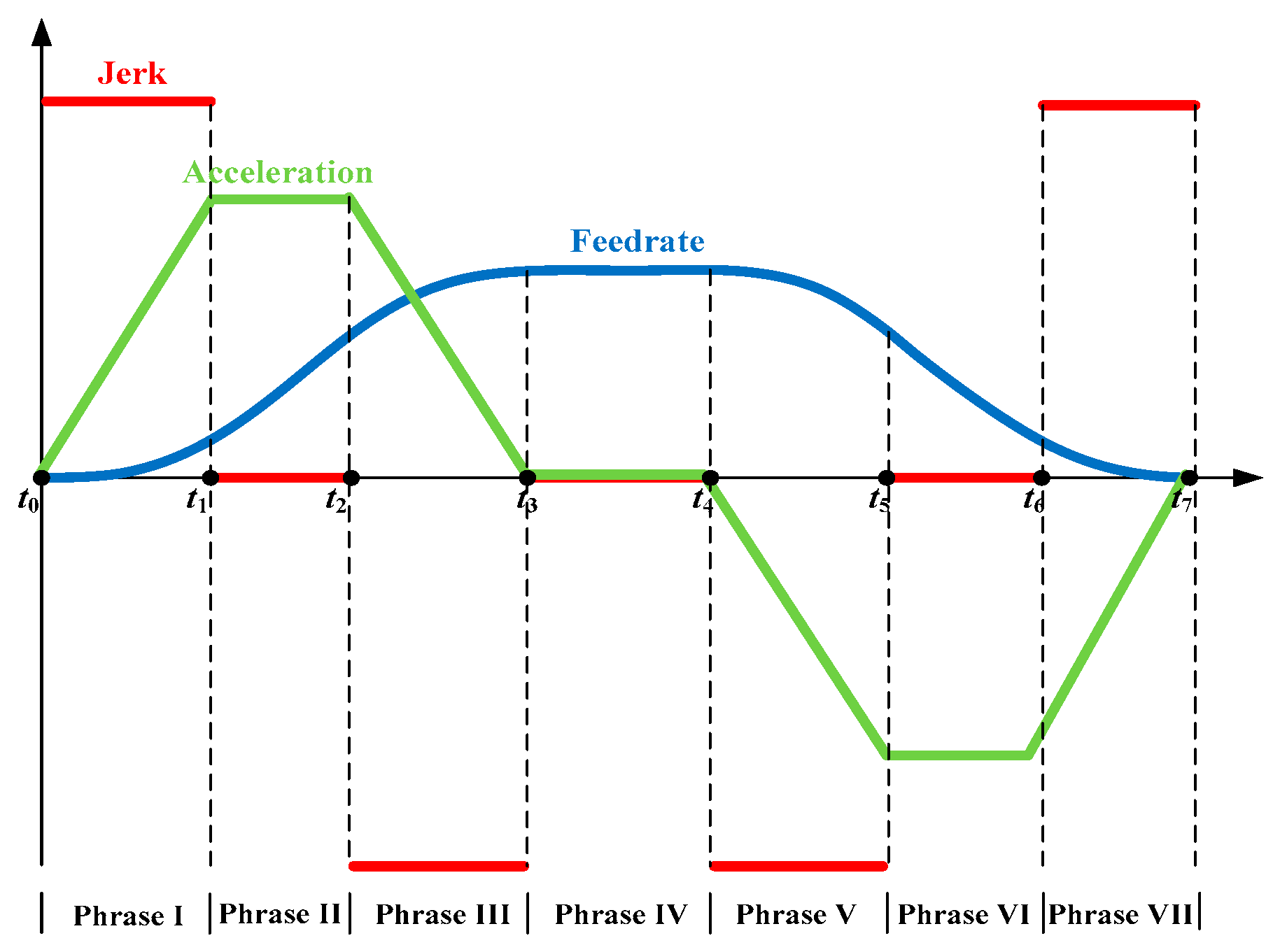
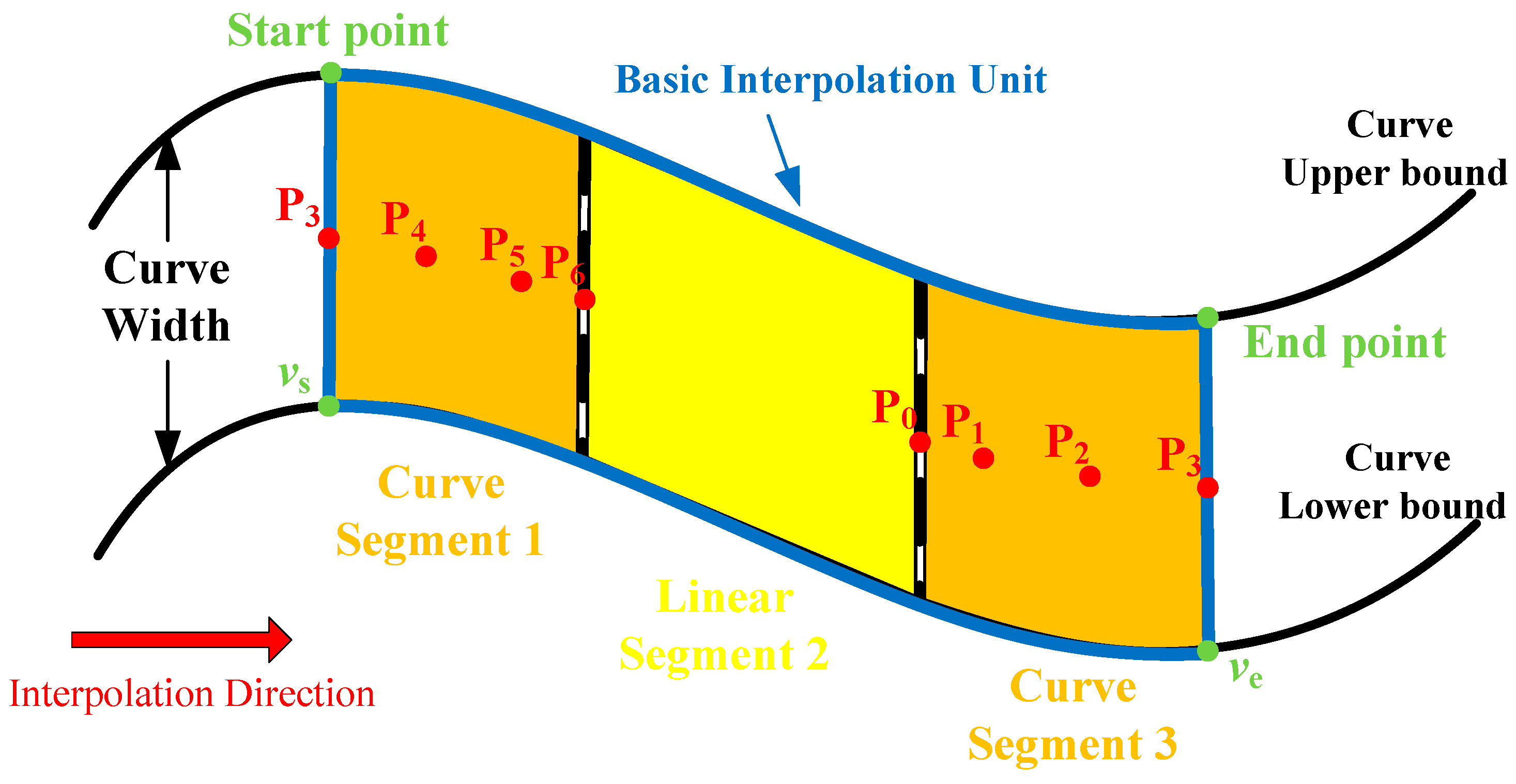
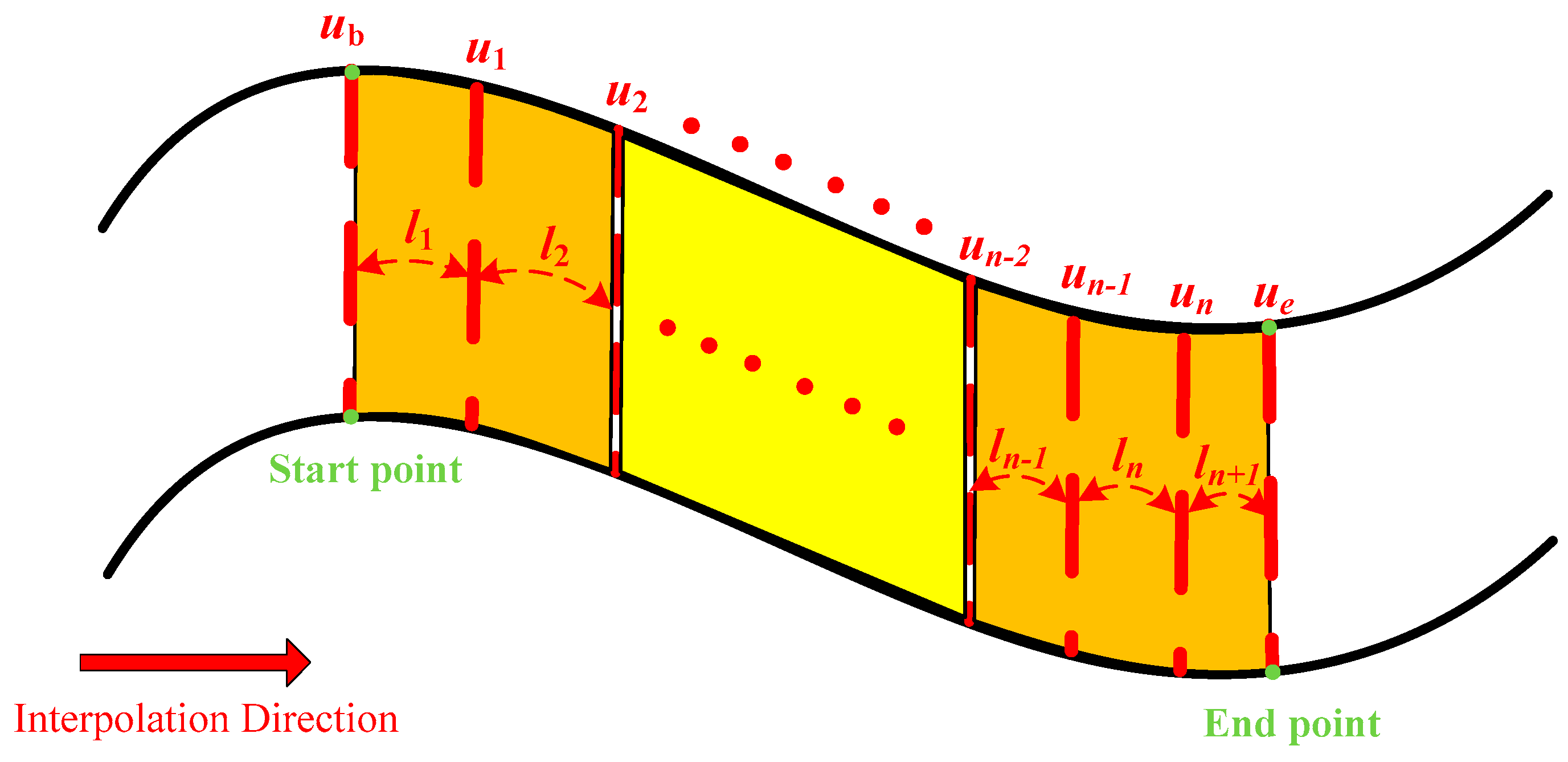
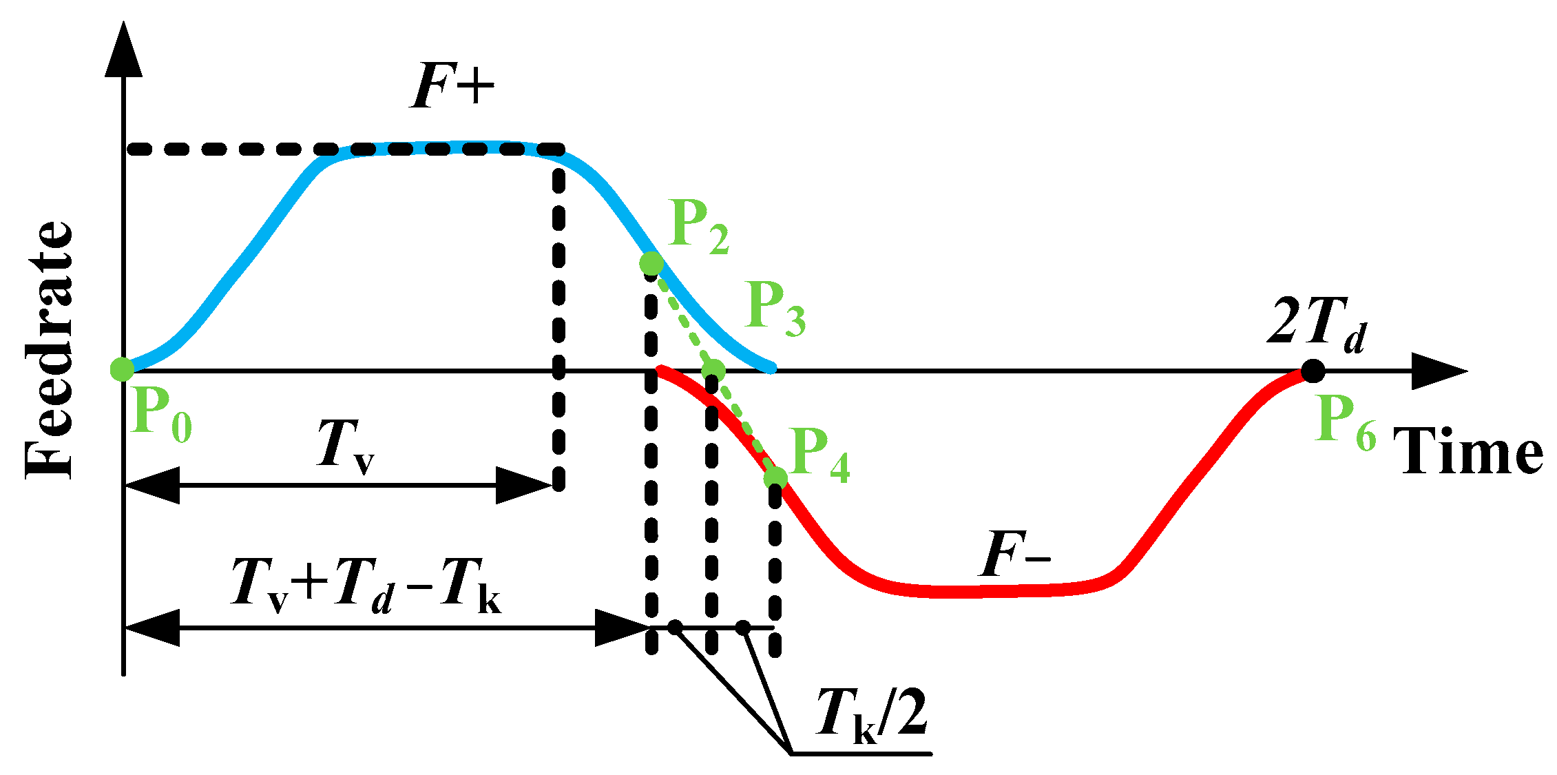
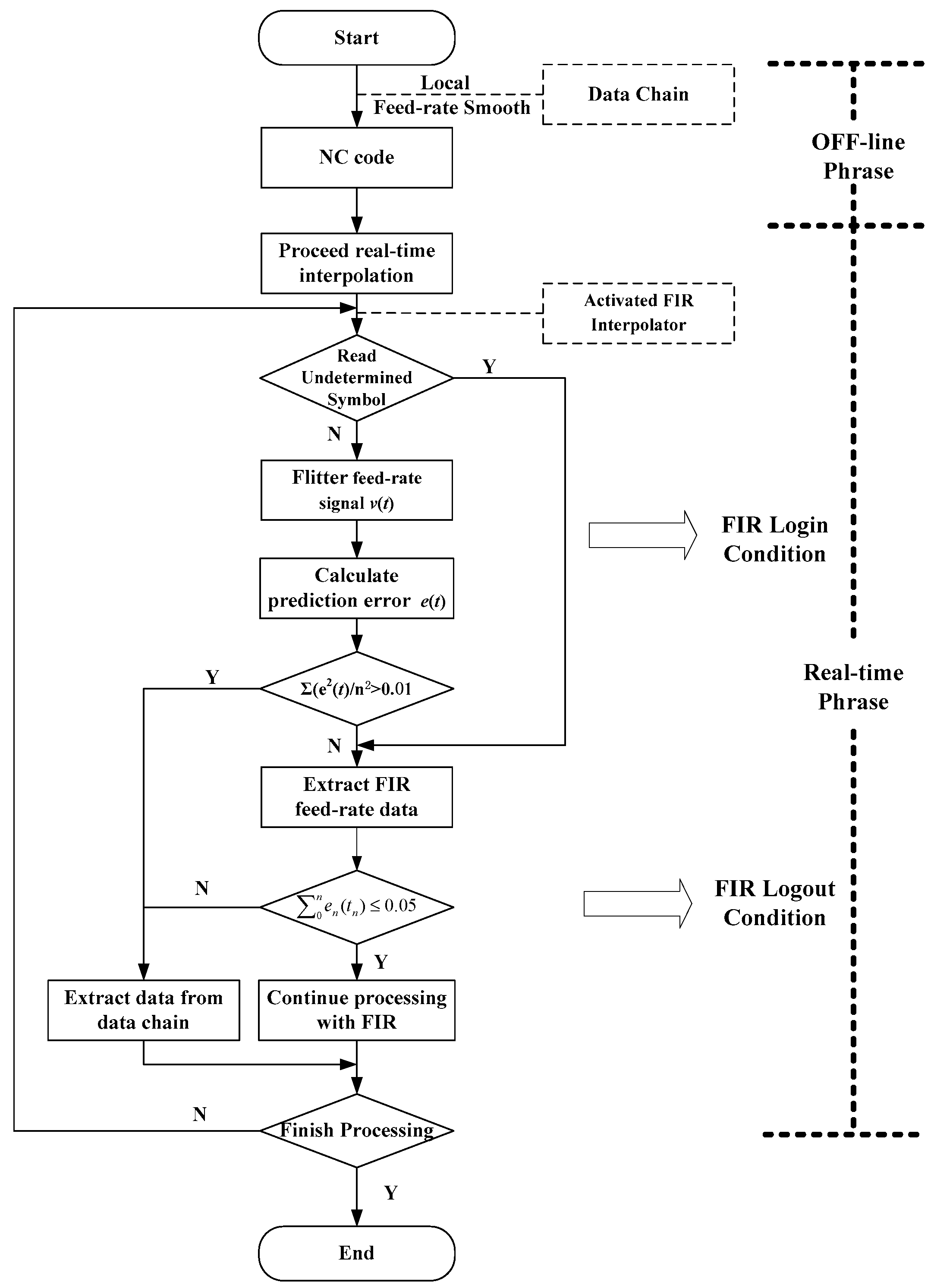
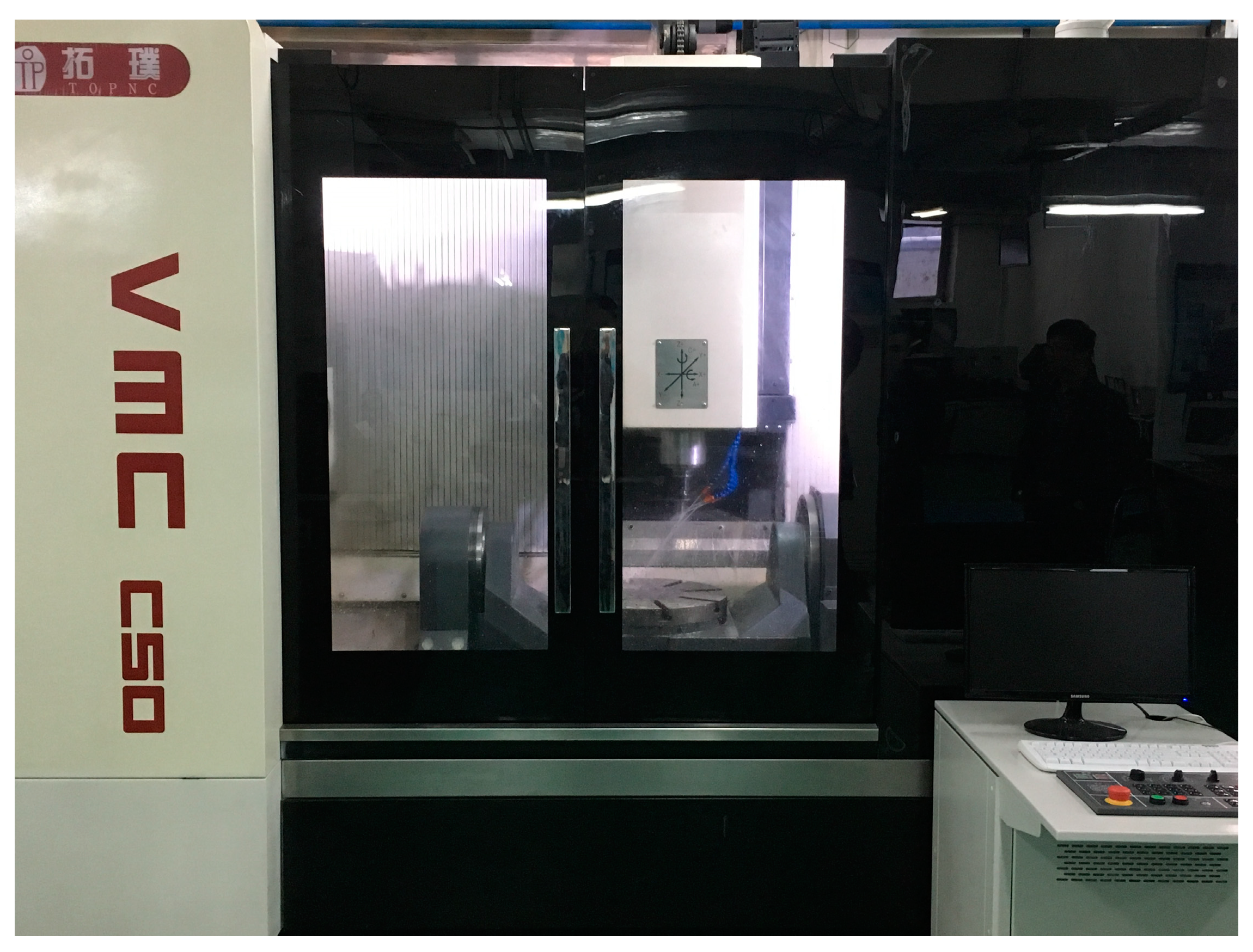
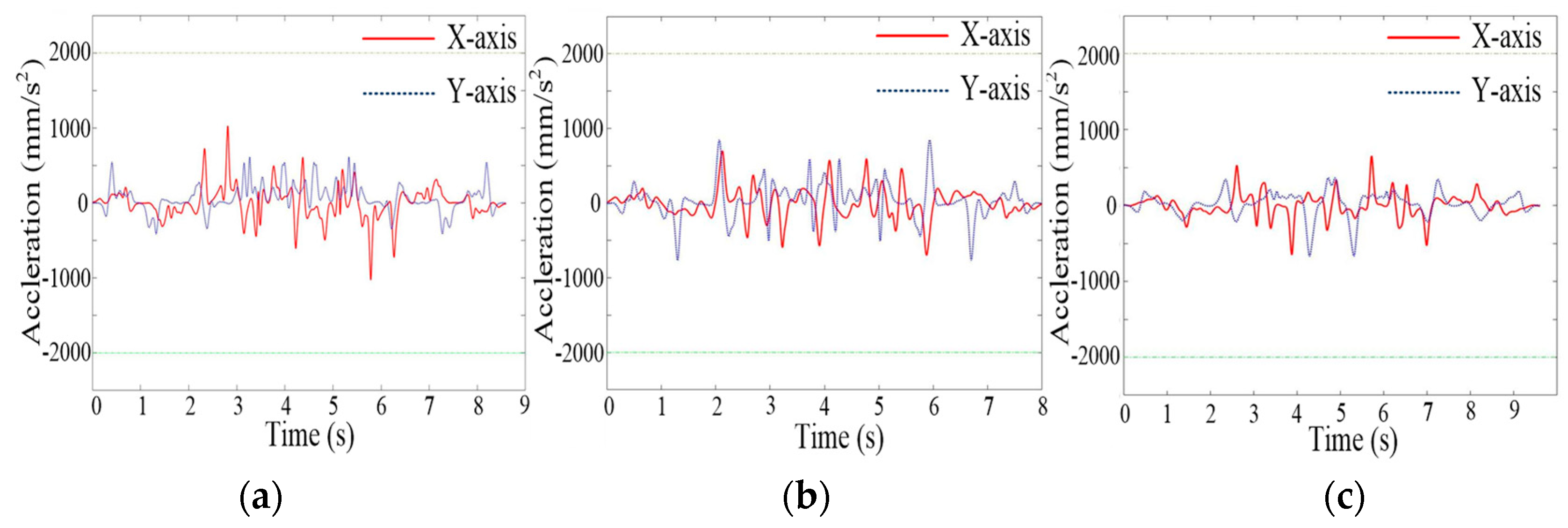
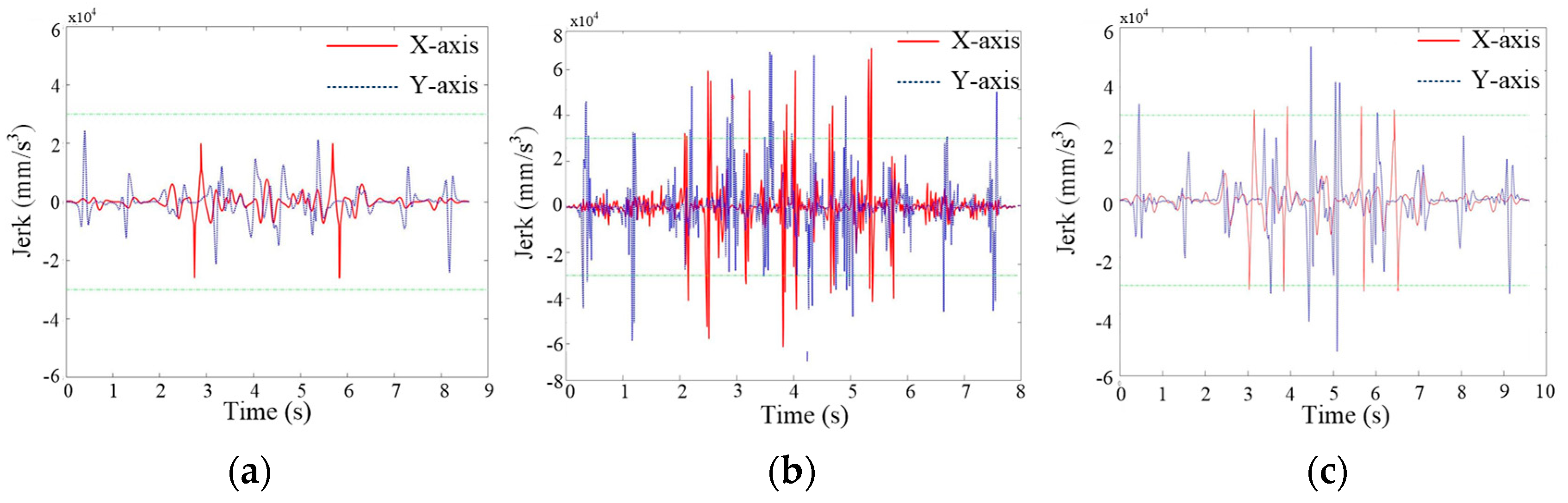
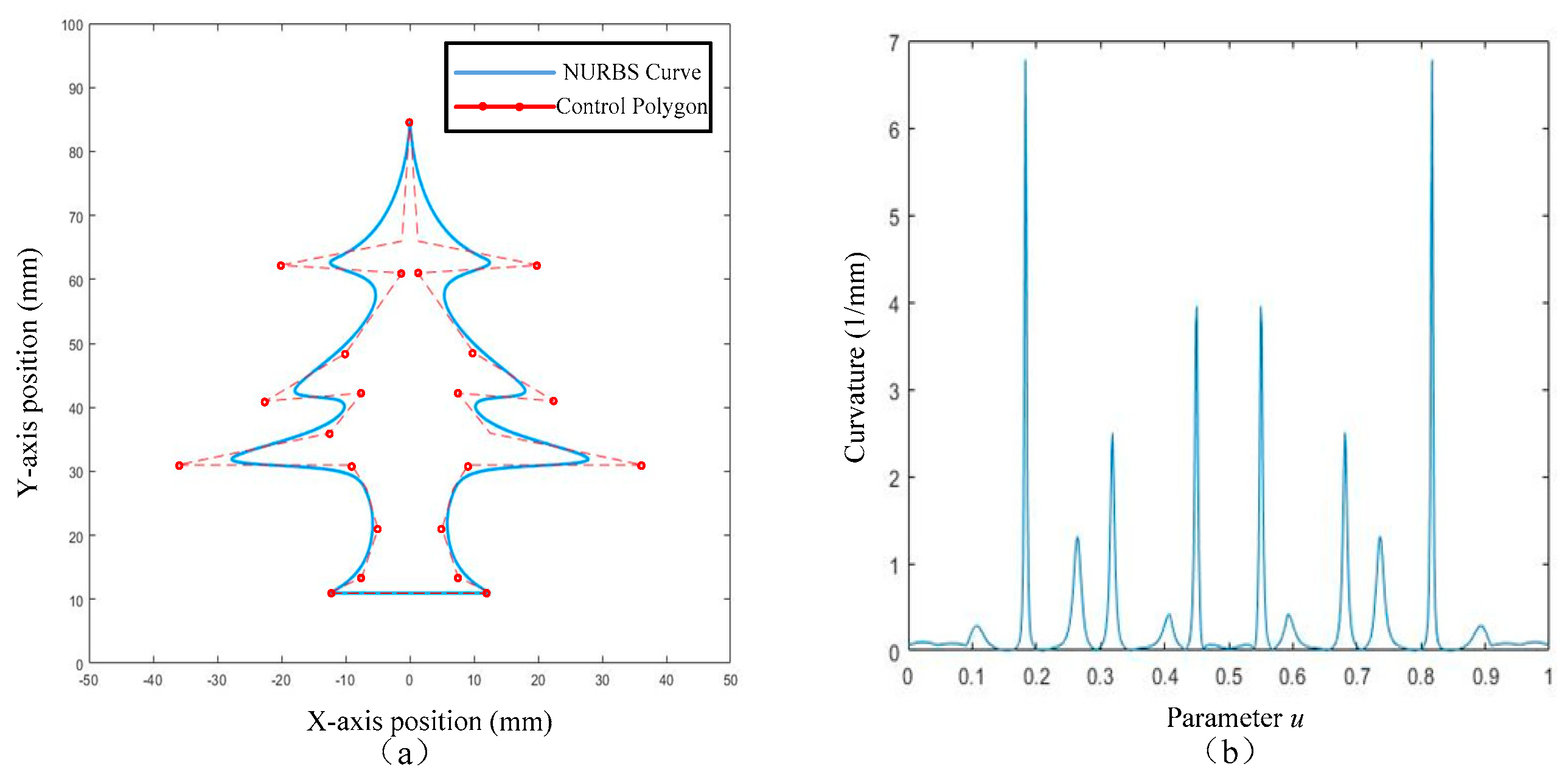
Table 1.
Simulation parameters.
| Parameter | Value | Unit |
|---|---|---|
| Interpolation period T | 1 | ms |
| Maximum chord error ςmax | 0.001 | mm |
| Maximum contour error εmax | 0.05 | mm |
| Maximum normal acceleration an,max | 950 | mm/s2 |
| Maximum tangential acceleration at,max | 2000 | mm/s2 |
| Maximum normal jerk Jn,max | 26,000 | mm/s3 |
| Maximum tangential jerk Jt,max | 30,000 | mm/s3 |
| Maximum feed rate fmax | 60 | mm/s |
Table 2.
Comparison of simulation results of the WM-shaped NURBS curve.
| Constraints | Typical Offline Method | Proposed Method | FIR Method |
|---|---|---|---|
| Maximum contour error (mm) | 4.12 × 10⁻⁴ | 4.08 × 10⁻⁴ | 3.27 × 10⁻⁴ |
| Maximum chord error (mm) | 6.24 × 10⁻⁴ | 5.87 × 10⁻⁴ | 5.17 × 10⁻⁴ |
| Maximum tangential jerk (mm/s3) | 30,000.00 | 30,000.00 | 30,000.00 |
| Maximum normal jerk (mm/s3) | 28,736.12 | 26,000.00 | 25,762.07 |
| Response time (us) | 25 | 38 | 102 |
| CPU occupancy rate (%) | 13 | 15 | 22 |
| Machining time (s) | 1.62 | 1.66 | 1.95 |
| Scheduling time (s) | 2.75 | 2.18 | \ |
| FIR interpolator intervention | No | No | Yes |
Table 3.
Processing parameters.
| Parameter | Value | Unit |
|---|---|---|
| Interpolation period T | 1 | ms |
| Maximum tangential acceleration at,max | 2000 | mm/s2 |
| Maximum tangential jerk Jt,max | 30,000 | mm/s3 |
| Maximum feed rate fmax | 60 | mm/s |
| Maximum chord error ςmax | 0.001 | mm |
| Maximum contour error εmax | 0.05 | mm |
Table 4.
Comparison of machining results of the butterfly-shaped NURBS curve.
| Constraints | Typical Offline Method | Proposed Method | FIR Method |
|---|---|---|---|
| Maximum contour error (mm) | 5.36 × 10⁻⁴ | 4.78 × 10⁻⁴ | 4.13 × 10⁻⁴ |
| Maximum chord error (mm) | 8.11 × 10⁻⁴ | 5.32 × 10⁻⁴ | 4.95 × 10⁻⁴ |
| Maximum X-axis jerk (mm/s3) | 73,164.00 | 21,715.27 | 31,742.69 |
| Maximum Y-axis jerk (mm/s3) | 69,214.15 | 23,654.46 | 51,782.83 |
| Response time (us) | 75 | 261 | 306 |
| CPU occupancy rate (%) | 14 | 23 | 29 |
| Machining time (s) | 8.05 | 8.43 | 9.52 |
| Scheduling time (s) | 6.39 | 4.57 | \ |
| FIR interpolator intervention | No | Yes | Yes |
Table 5.
The comparison results of contour errors in tree-shaped NURBS curve.
| Methods | Point 1 | Point 2 | Point 3 | Point 4 | Point 5 | Unit |
|---|---|---|---|---|---|---|
| Typical offline method | 0.0597 | 0.0498 | 0.0472 | 0.0661 | 0.0392 | mm |
| Proposed method | 0.0278 | 0.0314 | 0.0214 | 0.0473 | 0.0183 | mm |
| FIR method | 0.0219 | 0.0363 | 0.0593 | 0.0588 | 0.0365 | mm |
Table 6.
Comparison Results of machining indicators.
| Constraints | Typical Offline Method | Proposed Method | FIR Method |
|---|---|---|---|
| Response time (us) | 65 | 213 | 289 |
| CPU occupancy rate (%) | 14 | 19 | 25 |
| Machining time (s) | 375 | 392 | 465 |
| Scheduling time (s) | 5.11 | 3.92 | \ |
| FIR interpolator intervention | No | Yes | Yes |
Disclaimer/Publisher’s Note: The statements, opinions and data contained in all publications are solely those of the individual author(s) and contributor(s) and not of MDPI and/or the editor(s). MDPI and/or the editor(s) disclaim responsibility for any injury to people or property resulting from any ideas, methods, instructions or products referred to in the content. |
© 2024 by the author. Licensee MDPI, Basel, Switzerland. This article is an open access article distributed under the terms and conditions of the Creative Commons Attribution (CC BY) license (https://creativecommons.org/licenses/by/4.0/).
Share and Cite
MDPI and ACS Style
Zhou, X. An Adapted NURBS Interpolator with a Switched Optimized Method of Feed-Rate Scheduling. Machines 2024, 12, 186. https://doi.org/10.3390/machines12030186
AMA Style
Zhou X. An Adapted NURBS Interpolator with a Switched Optimized Method of Feed-Rate Scheduling. Machines. 2024; 12(3):186. https://doi.org/10.3390/machines12030186
Chicago/Turabian StyleZhou, Xiaoyang. 2024. "An Adapted NURBS Interpolator with a Switched Optimized Method of Feed-Rate Scheduling" Machines 12, no. 3: 186. https://doi.org/10.3390/machines12030186
Note that from the first issue of 2016, this journal uses article numbers instead of page numbers. See further details here.