Article

AC-Winding-Resistance Calculation of Toroidal Inductors with Solid-Round-Wire and Litz-Wire Winding Based on Complex Permeability Modeling †

1
School of Engineering, Newcastle University, Newcastle upon Tyne NE1 7RU, UK
2
Department of Electrical and Electronic Engineering, Pusan National University, Busan 46241, Republic of Korea
3
Robotics Institute of Non-Destructive Inspection, Pusan National University, Busan 46241, Republic of Korea
*
Author to whom correspondence should be addressed.
This paper is an extended version of our paper published in 2022 25th International Conference on Electrical Machines and Systems (ICEMS), Chiang Mai, Thailand, 29 November–1 December 2022.
Machines 2024, 12(4), 228; https://doi.org/10.3390/machines12040228
Submission received: 28 February 2024 / Revised: 23 March 2024 / Accepted: 27 March 2024 / Published: 28 March 2024
(This article belongs to the Section Electrical Machines and Drives)

Abstract

:
This paper has investigated a method for calculating the frequency-dependent winding resistance of toroidal inductor windings with Litz-wire as well as solid-round wire. The modified Dowell’s model is employed to address the effectiveness for inductor windings with the low and high filling factors. To overcome the limitation of this model, especially for a winding densely wound around the core, an alternative approach based on the complex permeability and iterative calculations is proposed. For the calculated AC-resistance factor of five inductors with different numbers of turns, layers with the same wire diameters are compared with that of FEA, and the three air-core toroidal windings are manufactured and tested within the frequency where the self-resonance can be neglected. The proposed model demonstrates the versality of the AC-resistance calculation of both solid- and Litz-wire windings within an error of 15% across a wide range of frequencies up to 1 MHz, compared with FEA.

1. Introduction

The recent advancement of wide band gap (WBG) semiconductors enables higher switching frequencies, expanding the frequency spectrum of the electric machines and magnetic components for power-conversion applications [1,2,3]. In particular, the increase in the switching frequency enables the downsizing of inductors, which have traditionally occupied a substantial volume in power electronics’ converters. However, along with increasing the frequency, alternating current (AC) losses in the winding result in both thermal issues and efficiency degradation. The design of high-frequency inductors should consider the loss density, as well as the power density, to mitigate undesirable temperature rises. Therefore, an accurate calculation of the frequency-dependent winding losses, referred to as ‘AC-winding losses’ across wide frequencies is imperative for the effective design and development of inductors [4].
The AC-winding losses comprise two primary contributions: the skin effect and the proximity effect. The skin effect refers to the uneven electric current density toward the surface of the wire, categorized into the strand-level and bundle-level skin effects. In stranded wires or a Litz-wire configuration, the strand-level skin effect arises from self-exciting currents due to unbalanced impedance among strands, exciting more net currents to outer strands. Therefore, careful consideration is required, especially when the Liz-wire is not well twisted. The proximity effect stems from eddy currents inside the wire, attributed to inter-turn and inter-wire magnetic fields. Normally, this effect typically dominates by increasing winding losses in multi-layer windings, accounting for a major component of AC-winding losses.
Numerous studies have proposed original and modified approaches to calculate the frequency-dependency of the winding losses, including the homogenization method based on the complex permeability [5,6,7,8,9], unit-cell simulations [10,11], and partial element equivalent circuit (PEEC) [12], as well as the hybrid method [13,14], and analytical models [15,16,17,18,19,20,21]. Sullivan et al. [5] and Gyselinck et al. [6,7] calculated the frequency-dependent complex permeability of a winding region based on finite element analysis (FEA). Igarashi et al. proposed closed-form expressions for the complex permeability and homogenization of a multi-turn winding based on the Ollendorff formula, obtaining frequency-dependent losses combined with FEA [8,9]. In [10], the unit-cell simulation is employed to obtain the equivalent complex permeability of round and rectangular wires in two transverse and longitudinal directions. The unit-cell simulation was applied to derive the high-frequency proximity effect for a Litz-wire coated with magnetic and conductive materials for megahertz frequency applications in [11]. For a Litz-wire, the twisted structure was precisely considered by using the magnetic field on cut sections of the wire for PEEC calculation in [12]. For the simplicity of calculations, the hybrid method can be used, which is the combination of an analytical formula of the AC resistance with FEA. This approach is preferred in the electric-machine applications with an acceptable accuracy and reduced computing time to take account of the complex geometry of electric machines [13,14]. However, the formula used for the hybrid method is very limited at low frequencies where the skin depth is larger than the wire size.
Conversely, analytical methods are efficiently used for axisymmetric windings such as planar windings, and transformer/inductor windings represented by a simple magnetic circuit. Acero et al. derived the analytical form of the Litz-wire planar winding for induction-heating applications [15]. This analytical form cannot reflect the reaction field from adjacent wires by considering the successive reactions, as observed in [16]. However, the approach used in [16] is rather complex, posing a limit to extending this approach in various winding configurations. For a simpler way, an iterative approach was proposed to consider the reaction field of the solid-wire winding [17].
The reaction field can be effectively considered for typical inductor and transformer winding with a simple analytical form. The densely wound wires in the winding can be equally seen as the equivalent of foil windings, so the Dowell’s approach can be directly applied [18,19]. However, this method has been used for the transformer windings where the turns in each layer exhibit the same structure. To overcome the limitation of the original method, some authors proposed an analytical formulation of AC-winding losses for a solid-round wire winding by modifying Dowell’s model to account for the layered structure of the toroidal inductor [20,21].
This article proposes a new calculation approach based on the complex permeability for AC-winding resistance in both solid and Litz wire toroidal inductors, which is an extended version from the author’s conference papers [22], providing more detailed explanations with experimental results. The round wire is considered to be an equivalent diamagnetic wire with complex permeability and zero electrical conductivity. Additionally, to address analytical inter-strand losses in Litz-wire configurations, the strands are homogenized based on the Ollendorff formula. To enhance the calculation of an inter-wire proximity effect (wire to wire) at higher frequencies, the magnetic fields originally calculated at each wire are corrected based on an iterative approach to exploit exact magnetic fields, including the reaction field by eddy currents.
The structure of the following article is organized as follows: In Section 2.1, Elizondo’s work is reviewed to update the methodology aimed at toroidal inductors and to discuss its validity [21]. The calculated results are compared with that of FEA with five inductors with the same core material and size but with different winding structures. In Section 2.2, the effectiveness of 1-D distributions of magnetic fields are discussed by analyzing the magnetic field and the contribution to AC resistance from loosely wound and densely wound wires around the air core and the magnetic core. In Section 3, the calculation method of both solid-round-wire and Litz-wire windings is proposed based on the complex permeability and homogenization, and the iterative approach is introduced to extend the approach to higher frequencies. In Section 4, the proposed method is employed to calculate AC resistance in the same inductor in Section 2, additionally with the Litz-wire windings. The results are compared with those of FEA and measurements. Finally, Section 5 concludes the paper and outlines future research directions.

2. A Literature Review of Winding Loss Calculation in Toroidal Inductor Windings

2.1. Modified Dowell’s Model

Traditionally, Dowell’s model has been widely adopted in the design of magnetic components due to its simplicity and ease of optimization for finding the optimal winding layout. However, Dowell’s model has limitations in its applicability, attributed to its origins in axisymmetric transformer windings with foil conductors. This model assumes densely wound windings immersed in a one-dimensional (1-D) magnetic field distribution, making it less suitable for models deviating from standard transformer windings and densely wound configurations. To overcome the limitation from the former assumption, Elizondo et al. modified the original Dowell’s model to address the layer-by-layer structure of the toroidal inductor, as depicted in Figure 1 [21].
Figure 1 illustrates the parameters in the inductor structure, where the inductor consists of m-layer windings, with each layer comprising nk-turn wires in the k-th layer. The wire utilized in the winding can be a solid round wire, a Litz wire, or a foil wire; however, the focus in this article is the solid-round and Litz-wire windings. The packing factor kf,k represents the ratio of the area occupied by all wires to that of the winding window in the k-th layer. The toroidal winding exhibits distinct parameters in the inner and outer cores, as well as each layer. Consequently, the winding resistance in the k-th layer, formulated by Elizondo in [21], is given by the following:
R w , k = k M L T k σ π r c 2 n k sinh 2 k + s i n 2 k cosh 2 k c o s 2 k + 2 j = k + 1 m n j 1 n k + 1 sinh k + s i n k cosh k c o s k
where MLTk is the mean length per turn, and Δk is a normalized frequency for an equivalent winding window in the k-th layer, given by the following:
Δ k = w c π f μ 0 σ c k f , k = n k r c 2 2 R k π f μ 0 σ c k f , k  
where Rk indicates the mean radius of the wire located in k-th layer, f is the frequency, μ0 is the permeability of air, and σc is the electrical conductivity of a copper wire. This unitless value is normalized by the classical skin depth and the layer width wc. The total winding resistance Rw can subsequently be obtained by summing the winding resistance in the inner and outer section as well as across all layers, and the AC resistance factor Fw,ac, which indicates the increased ratio from the DC winding resistance Rdc, is written as the following:
F w , a c = R w R d c = 1 R d c k = 1 m R w i , k + R w o , k .  
Here, Rwi,k and Rwo,k are the winding resistance for the inner and outer section of the k-th layer, respectively. Fw,ac does not include the exact length along the 3-D winding path, and the exact AC-winding resistance can be obtained by using Fw,ac to scale the measured DC winding resistance, assuming the AC effects are the same across all winding regions.
To demonstrate the effectiveness of the model, five case study models with the different numbers of turns, layers, while maintaining the wire radius, core size, and material are considered. The AC-resistance factors of each inductor model are compared with those obtained from FEA computed by COMSOL Multiphysics, as presented in Figure 2. The inner and outer diameters, as well as the height of a magnetic core, is 23.57 mm, 14.4 mm, and 8.89 mm, respectively. The wire diameters are 1.45 mm (AWG 15) and 1.51 mm, including an insulation layer, respectively. The electrical conductivity of the wire is set as 58 MS/m at the temperature of 25 °C. The relative permeability and conductivity in the FEA model are set to 60 and 0, respectively.
The AC-resistance factors of the five inductors are calculated and compared with those obtained from FEA, as summarized in Table 1. Inductor #1 to #4 features a single- layer winding with increasing packing factors, and Inductor #5 employs a double-layer winding configuration. The frequency where the classical skin depth equals the wire radius is 8.3 kHz, with the skin depth decreasing to 3.5 times smaller than the wire radius at 100 kHz and 11 times smaller at 1 MHz. It is worth nothing that the frequency of 1 MHz is aimed at for demonstrating the method’s capability, limiting a scenario to the increment due to eddy current losses, although, in practical scenarios, self-resonance due to parasitic capacitance will occur and increase the equivalent resistance much higher [23].
In Figure 2a,b, the results demonstrate that the modified Dowell’s model exhibits a notable increase in the winding resistance for Inductor #2 and #3, beginning at 100 kHz, with AC-resistance factors of 2.72 and 3.88, respectively. The error reaches 31.16% and 24.70% at 1 MHz, indicating an overestimation of the winding resistance. In contrast, the calculated resistance factor of Inductor #5 in Figure 2c closely aligns with it, with deviations of 6.83% at 100 kHz and −0.75% at 1 MHz, respectively. This method shows improved agreement for the double-layer winding and windings with higher packing factors. Notably, the discrepancy in this method’s accuracy is attributed to the winding layout, particularly in the case of Inductor #2 and #3, where a loosely wound configuration leads to a magnetic field distribution that cannot be assumed to be 1-D in Figure 3b.

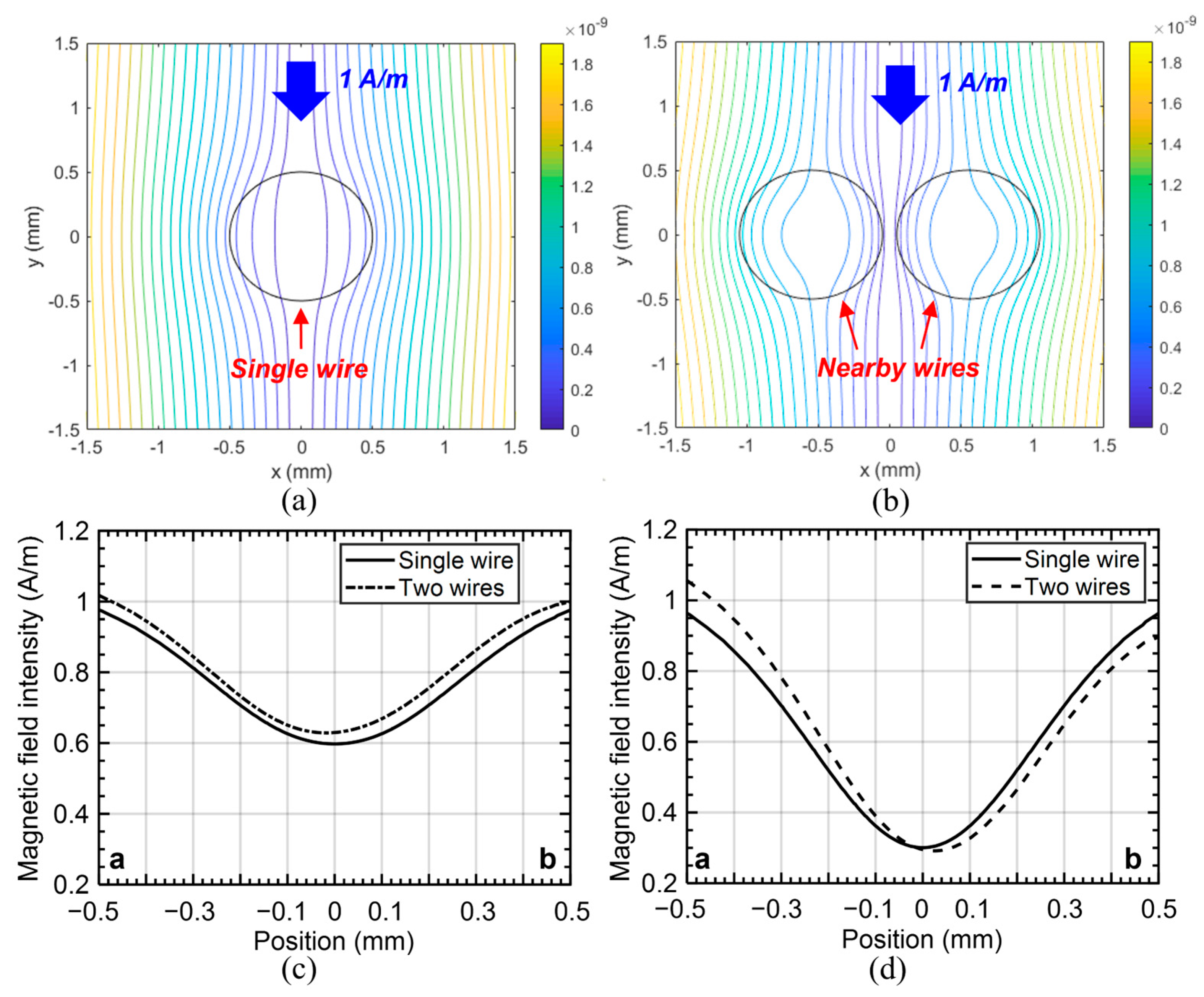
2.2. The Magnetic Field in the Winding and Its Contribution on the AC Winding Resistance

The accurate determination of the distribution and strength of magnetic fields is crucial for calculating AC-winding resistance. In Figure 3, the magnetic field distribution is highly influenced by two factors: the packing factor, which indicates how densely the wires are wound, and the adjacent magnetic core, deviating from the 1-D magnetic field.
Initially, the 1-D magnetic field distribution in the azimuthal direction used in the modified Dowell’s model is calculated based on Ampere’s law, assuming the continuous current distribution in each layer. However, actual inductors exhibit a discrete current distribution, especially in loosely wound windings, leading to deviations from the ideal 1-D distribution, as depicted in Figure 3a,b compared to those in Figure 4c,d. Furthermore, the winding in the outer section with lower packing factors results in a more 2-D distribution.
Figure 4 illustrates the azimuthal direction of magnetic fields along the same central radial position of wires (orange circles), depicted as the black dashed line in Figure 3a. Despite the small number of turns, the magnetic field can be approximated as a 1-D distribution and a constant value in the air-core winding. The fluctuation in the field distribution is primarily due to the internal field of each wire, which can be independently considered to bethe skin effect. However, as depicted in Figure 3a,b as well as Figure 4a,b, significant fluctuations occur when the wires are loosely wound around the magnetic core. This is attributed to the susceptibility of the magnetic field on the interface of the magnetic media to the radial direction, perpendicular to the core’s boundary. Conversely, densely wound cores, as shown in Figure 4c,d, justify the validity of Equation (1), where a 1-D magnetic field distribution in each layer is defined based on Ampere’s law.
Figure 5 decomposes the winding resistance into DC resistance and AC resistance, comprising contributions from the skin effect and proximity effect. Inductor #1 and #2, characterized by lower packing factors (below 20%), exhibit a lower contribution of the proximity effect compared to the skin effect, as shown in Figure 5a,b. Given that the AC resistance due to the skin effect can be accurately calculated using the analytical formulation of the round wire, the accuracy of the AC resistance for loosely wound cores is less sensitive to the magnetic field calculation for the proximity effect. However, the contribution of the proximity effect increases with the number of turns, as depicted in Figure 5c,d. Nonetheless, for Inductor #3, #4, and #5 with higher packing factors (over 50%), the assumption of a 1-D magnetic field along the azimuthal direction, as shown in Figure 4c,d, remains acceptable. Therefore, the accurate calculation of the magnetic field along the angular position is less significant, and the initial assumption of a 1-D magnetic field remains valid.

3. Complex Permeability Approach for AC-resistance Calculation

This section describes the concept of the complex-permeability approach for calculating the AC resistance of both solid-round-wire and Litz-wire configurations. Additionally, the homogenization approach is adopted to extend the analytical solution from a solid round wire to a Litz wire.

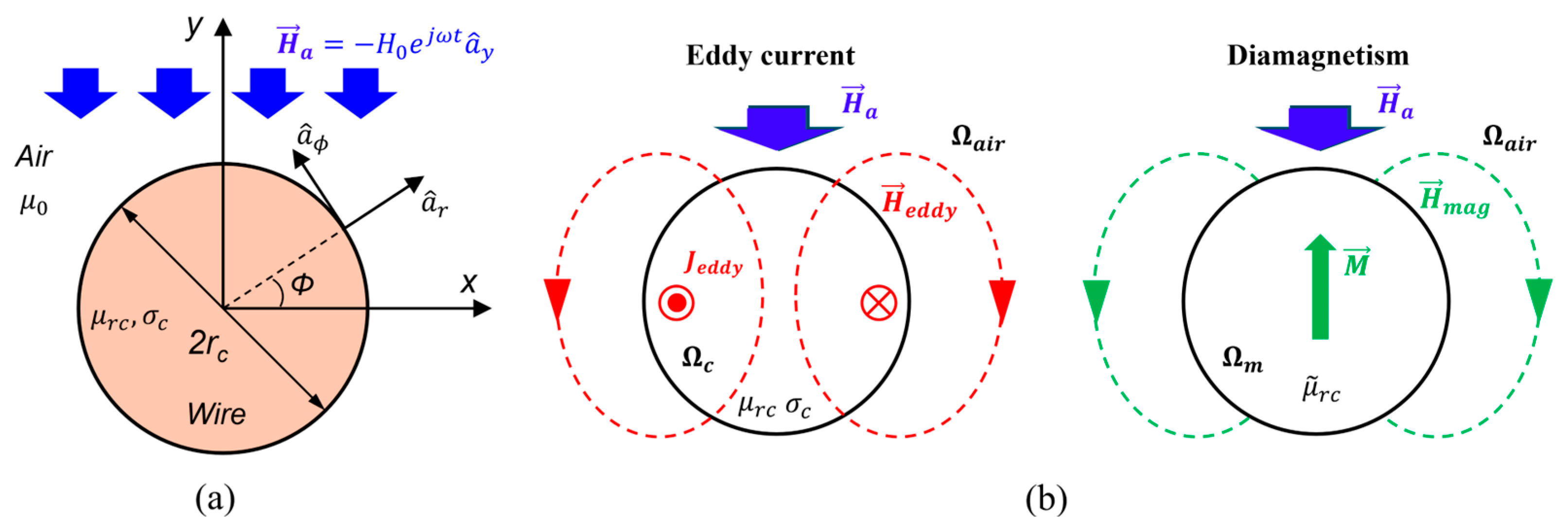
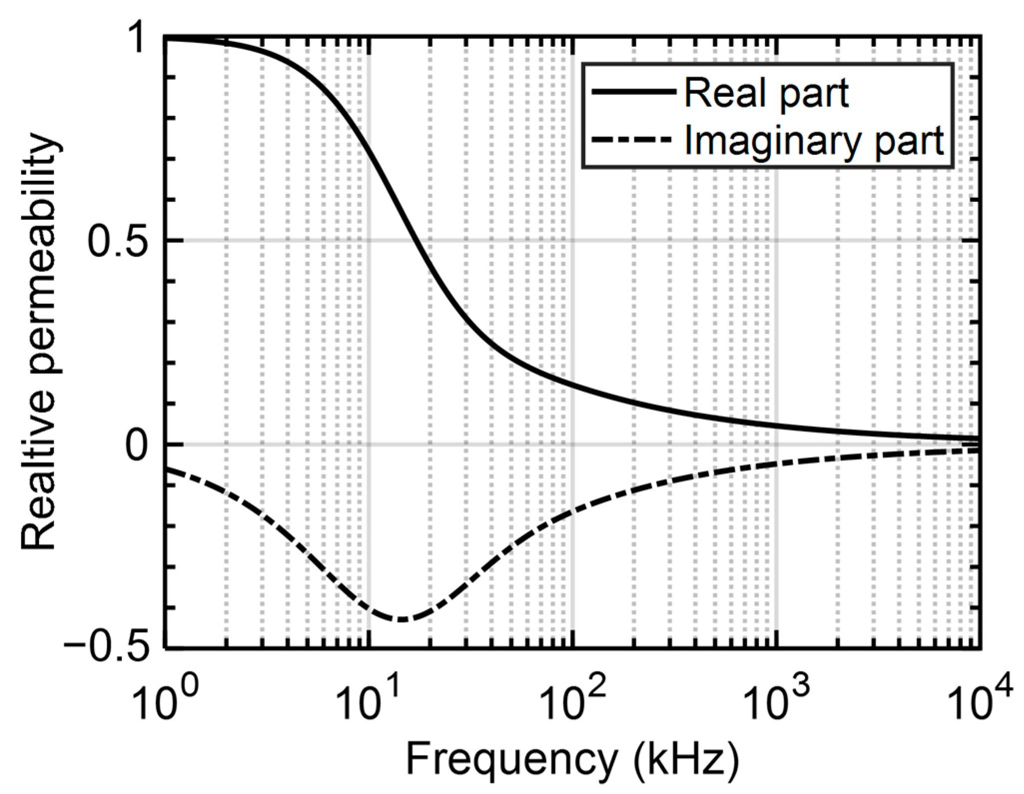
3.1. Complex Permeability of a Solid Round Wire

The concept of complex permeability is commonly utilized in modeling the hysteresis losses of magnetic cores in the frequency-domain analysis. The imaginary part of the complex permeability indicates the loss due to the time-harmonic magnetic field, and its real part contributes the magnetic energy. In this article, this concept is adopted to derive the equivalent expression of the eddy current loss, enabling us to simplify the analytical expression for both the solid-round-wire and the Litz-wire configurations.
In Figure 6a, a round wire immersed in a uniform magnetic field with amplitude Ha and the angular frequency ω in y-direction is depicted. The wire, with radius rc, electrical conductivity σc, and relative permeability μrc, exhibits an eddy current loss due to the proximity effect. Solving Maxwell’s quasi-static differential equation yields the following expression for eddy current loss:
P p r o x = l w π 2 k c r c σ c R e j 1 / 2 J 0 j 3 / 2 k c r c J 1 * j 3 / 2 k c r c J 0 j 3 / 2 k c r c 2 H a 2
where lw is the wire length, J0 and J1 are the Bessel function of the first kind of orders 0 and 1, respectively, and * denotes the conjugate operator. The coefficient kc is defined as the following:
k c = ω μ 0 μ r c σ c .
The equivalent representation can be expressed based on the similarity of the conductive wire and a magnetic wire, as shown in Figure 6b. To obtain the equivalent complex permeability of the round wire, the eddy current loss in Equation (4) is formulated as the real part of the complex power:
P e q = R e j ω 2 μ 0 μ ~ r c H e 2 π r c 2
where μ ~ r c is the complex permeability of the wire and He is the magnetic field in the wire. The magnetic field He can be expressed in terms of the applied magnetic field Ha by using a demagnetizing field as follows:
H e = 1 1 + N d ( μ ~ r c 1 ) H a .
Here, Nd is the demagnetizing constant, which only depends on the shape of the wire and is set as 0.5 for a round wire. Substituting He into Equation (6) and solving for μ ~ r c based on the identity relation between Equations (4) and (6), the equivalent complex permeability of the round wire is obtained as the following:
μ ~ r c = μ r c J 1 j 3 / 2 k c r c j 3 / 2 k c r c J 0 j 3 / 2 k c r c J 1 j 3 / 2 k c r c .  
The complex permeability of the wire (rc = 0.725 mm, σc = 58 S/m, and μrc = 1) is illustrated in Figure 7. The real part decreases with increasing frequency, reflecting the shielding effect due to the magnetic field induced by eddy currents. Conversely, the imaginary part, having a negative sign, describes the dissipated power due to the AC magnetic field.

3.2. Complex Permeability of a Litz-Wire

The Litz wire, composed of tens to thousands of strands, presents a challenge in considering the interaction among strands when calculating AC resistance. To address this challenge, the homogenization approach is adopted, as illustrated in Figure 8. This approach transforms micro-scale particles (strands) arrayed periodically into a macro-scale domain (wire). It is particularly effective when the size of the macro-scale domain (rc) is much larger than that of the square cell (w) dividing the region of each micro-scale particle. In an ideal Litz wire, the source currents are uniformly distributed in each strand due to the balanced impedance from the twisted structure. Therefore, the homogenization approach simplifies the consideration of all strands by transforming individual strands into an equivalent solid wire.
The analytical complex permeability of the Litz wire, derived from the complex permeability of a strand, is defined by the Ollendorff formula as [24] the following:
μ ~ r c = 1 + β μ ~ r s 1 1 + N d 1 β μ ~ r s 1
where
      β = n s r s 2 r c 2 .
Here, β represents the filling factor, rs is the diameter of a strand, and ns is the number of strands. Despite strands being more randomly arranged and unable to be divided into square cells, the arrangement’s effect is deemed insignificant based on previous studies. Therefore, in this article, β in Equation (9) represents the ratio of the wire’s surface area usage to the outer diameter of the Litz-wire bundle, as defined in Equation (10).
The proximity effect in the Litz wire can be divided by the internal-proximity effect and the external proximity effect, induced due to the self-induced magnetic field generated by Litz-wire current Ic and the magnetic field from nearby wires, respectively. The AC resistance due to the internal-proximity effect can be calculated by the internal magnetic field, simply given by Ampere’s law [24]:
H a = H i n t = r I C 2 π r c 2             ( 0 < r r c ) .
Substituting Equations (9) and (11) into (6) yields a simplified form of the AC resistance due to the internal-proximity effect as follows:
R p r o x _ i n t n s ω μ 0 l w 8 π I m μ ~ r c .
Additionally, the contribution of the external proximity effect to the AC resistance of the Litz wire is expressed as the following:
R p r o x _ e x t = R e j ω μ 0 μ ~ r c H a 1 + N d ( μ ~ r c 1 ) I c 2 π l w n s r s 2 β   .
This form can be utilized for the solid round wire, where ns = 1, rs = rc, and β = 1.

4. Iterative Calculation Approach for Higher-Frequency AC-Resistance Calculation

The analytical form of the AC resistance due to the proximity effect in the previous section considers a single wire isolated from other wires, neglecting the interaction among adjacent wires. This section investigates the effect of the magnetic field produced by eddy currents in nearby wires on the AC resistance and proposes the iterative calculation approach to improve the accuracy of the calculation.

4.1. The Effect of the Magnetic Field Induced by Eddy Currents

To analyze the influence of a nearby wire, a case study is conducted using FEA, as depicted in Figure 9. Two wires with a diameter of 1 mm are subjected to a uniform magnetic field of 1 A/m in the y-direction. The wires and boundaries in Figure 9 are not an actual scale, and the boundaries are too far from the wires to neglect their effects on the wires. The net current is set to zero to prevent circulating currents between the two wires. Magnetic fields and eddy current losses are calculated 0.05 mm away from the top of the wire at different frequencies and compared with those obtained using a single wire.
Figure 10a,b illustrate the flux line of the single wire and two wires within a square range of 1.5 mm at frequencies of 100 kHz. The presence of an adjacent wire alters the flux lines compared to those of the single wire. Consequently, the eddy current loss in the wire deviates from the AC resistance derived based on a single wire due to nearby wires. Additionally, the ratio of the wire radius to the skin depth, referred to as the normalized frequency, is 2.39 at 100 kHz and 7.57 at 1 MHz. This indicates that the eddy currents and their reaction field become more substantial and opposite in phase to the applied magnetic field unlike lower frequencies, where the normalized frequency is below 1. Figure 10c,d compare the magnetic field distribution between the single wire and two wires in the y-direction at 100 kHz and 1 MHz, respectively. The applied magnetic field is significantly influenced by the reaction field induced by eddy currents in wires, and its impact exhibits a different trend at these two frequencies. At 100 kHz, the adjacent wire can decrease the reaction field applied to the wire, but the magnetic field far from the adjacent wire oppositely increases the reaction field, as shown in Figure 10d.
In Figure 11, eddy current losses in the wire for the single wire and two wires are presented, and neglecting nearby wires can result in increasing errors as the frequency increases. Therefore, to accurately predict the AC resistance across a broad spectrum of frequencies, especially when the wire size is much larger than the skin depth, these limitations should be addressed in the calculation methodologies.

4.2. Iterative Calculation Approach

To include the reaction field from adjacent wires, the applied magnetic field should be corrected by considering the interaction among wires. While this effect is inherently included in FEA, an additional method is necessary for an analytical approach. In this article, an iterative calculation approach is employed to calculate the AC resistance more accurately at higher frequencies. This approach, previously validated for planar and helical coils by the authors, is extended to the toroidal winding structure [24].
The concept of the iterative approach is illustrated with wires with n-turns, as depicted in Figure 12. The position of each wire is expressed in cartesian coordinates (X, Y), and local coordinates are defined at the center of each wire. Initially, the applied magnetic field at the k-th wire is calculated at the central position of each wire and denoted as H k ( 0 ) , where the superscription and subscription represent the number of iterations and the wire number, respectively. Subsequently, the magnetic field produced by the eddy current in the k-th wire is calculated at the position of the other wires. The reaction field of the round wire with the complex permeability can be obtained by solving the Poisson’s equation:
2 V m = 1 μ 0 μ ~ r c · M .
Here, V m is the magnetic scalar potential and M is the magnetization in the wire. Solving Equation (14) with the wire geometry depicted in Figure 6, the magnetic scalar potential can be represented as the following:
V m = r c 2 2 r M · a r
where M is a function of the permeability and applied magnetic field:
M = μ ~ r c 1 1 + μ ~ r c 1 N d H a .  
Substituting Equation (16) into (15) and transforming the scalar potential to the magnetic field produced by the j-th wire at the i-th wire yields the reaction field corresponding to the applied magnetic field:
H e X , i j = r c r i j 2 μ ~ r c 1 μ ~ r c + 1 H X , j 0 cos 2 ϕ i j sin 2 ϕ i j + 2 H Y , j 0 c o s ϕ i j s i n ϕ i j
H e Y , i j = r c r i j 2 μ ~ r c 1 μ ~ r c + 1 2 H X , j 0 c o s ϕ i j s i n ϕ i j + H Y , j 0 cos 2 ϕ i j sin 2 ϕ i j
where rij is the distance from the j-th wire to i-th wires, c o s ϕ i j and s i n ϕ i j are defined at the position of each wire as follows:
r i j = X i X j   2 + Y i Y j   2  
c o s ϕ i j = X i X j   X i X j   2 + Y i Y j   2 , a n d   s i n ϕ i j = Y i Y j   X i X j   2 + Y i Y j   2
The reaction field calculated at each wire can be superimposed to obtain the reaction field, subsequently defined as the k-th applied magnetic field. This magnetic field is repeatedly calculated by updating the magnetic field at the next step to the sum of the reaction field from near wires. The reaction field becomes converged within several steps due to its dependence on the square of the distance between wires at each iteration. Therefore, the iteration can be terminated when the convergence satisfies the predefined criteria. The magnetic fields from the initial step to the last step are added to determine the magnetic field with consideration of the reaction field.
Figure 13 presents the effectiveness of the iterative approach to consider the AC effects due to the proximity effect at higher frequencies. The analytic calculation using Equation (13) without iterations is called a ‘single calculation’, leading to an error of 24% and 38% at 100 kHz and 1 MHz, respectively, whereas the iterative method exhibits an error of 1.5% and 9% at the same frequencies.

4.3. AC-Resistance Calculation for a Toroidal Inductor Winding

To extend the methodology to a toroidal winding configuration. the proposed calculation is based on the solution of a round wire and can be modified using the complex-permeability approach outlined in our previous work [24]. The winding loss due to the skin effect can be obtained by
R s k i n = k s l w 2 π σ c n s r s R e j 3 / 2 J 0 j 3 / 2 k s r s J 1 j 3 / 2 k s r s
where ns = 1, rs = rc and ks = kc for the solid round wire. For the Litz wire, the internal-proximity effect should be additionally considered by Equation (12).
To substitute the magnetic field Ha into Equation (13), the magnetic field in the winding section in Figure 1 is calculated by Ampere’s law, expressed as the following:
H i , ( k ) = I c 2 π R i , k j = k + 1 m n j + n k R i , k R 1 , k 2 R 2 , k R 1 , k 2     f o r   t h e   i n n e r   w i n d i n g   s e c t i o n .
H o , ( k ) = I c 2 π R o , k j = k m n j n k R o , k R 1 , k 2 R 2 , k R 1 , k 2     f o r   t h e   o u t e r   w i n d i n g   s e c t i o n .  
Here, R 1 , k is the mean radius of the k-th layer, R 1 , k and R 2 , k are an inner and an outer radiuses of the k-th layer, respectively, and can be written as the following:
R 1 , k = R i , k w c / 2   a n d     R 2 , k = R o , k + w c / 2 .  
The contribution of the external proximity effect to the AC resistance can be formulated by substituting the magnetic field H ( k ) ( H i , ( k ) or H o , ( k ) ) into Equation (13).
R p r o x _ e x t = k = 1 m R e j ω μ 0 μ ~ r c , k H ( k ) 1 + N d ( μ ~ r c , k 1 ) I c 2 π l w n s r s 2 β k   .  
where βk, μ ~ r c , k , and H ( k ) are the parameters which can influence the AC resistance, so these should be defined according to the layers, inner section, and outer section of the winding. Finally, the AC resistance can be obtained by summing Equations (12), (21), and (25) for the Litz-wire winding, and Equations (12) and (25) for the solid-round-wire winding.

5. Simulation and Measurement

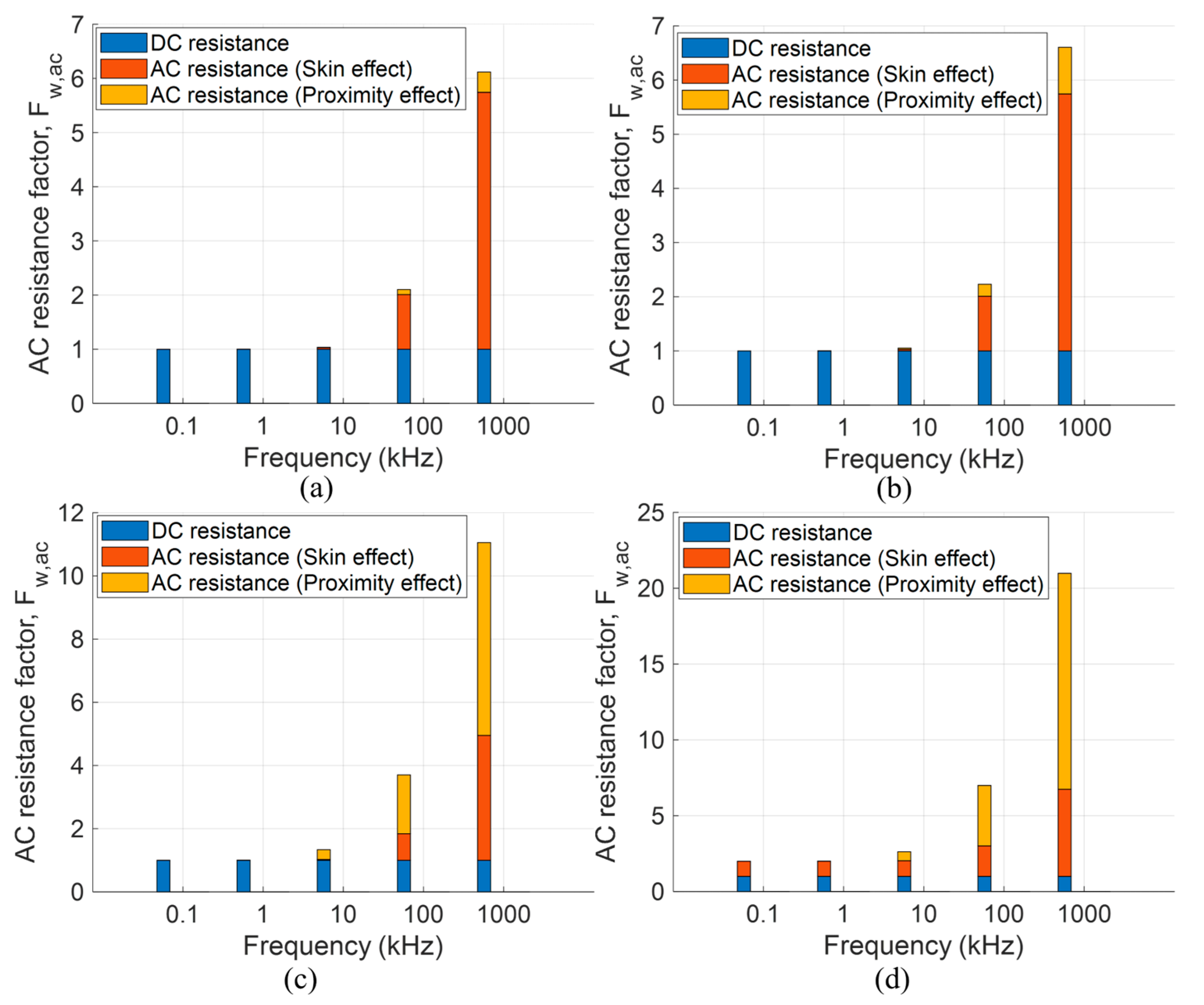
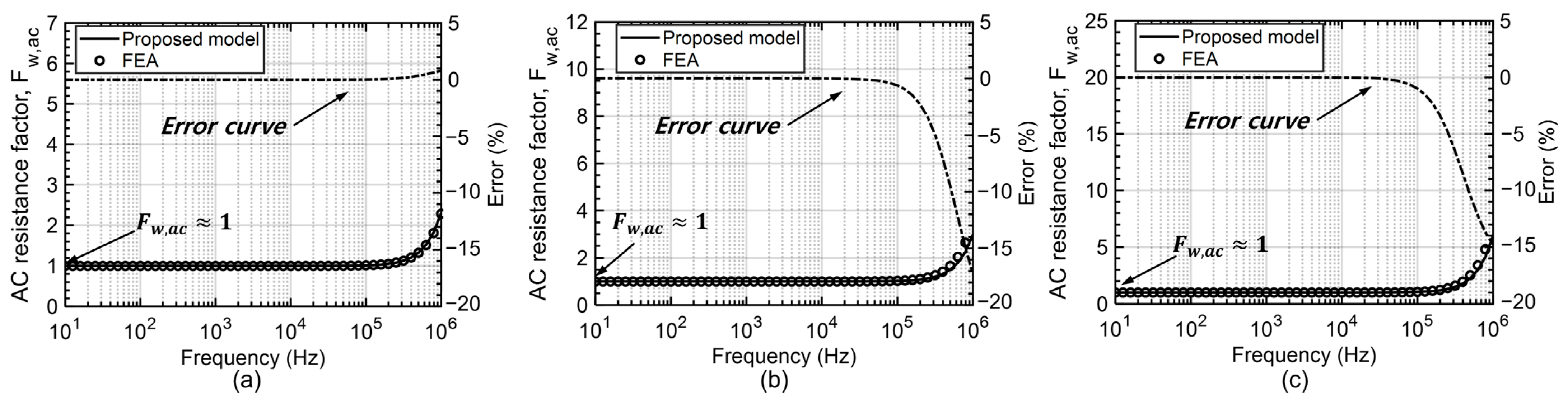
5.1. Calculation Results

The proposed approach has been applied to calculate the AC-winding-resistance factor for the five inductors, as described in Table 1. Additionally, the Litz-wire winding has been incorporated and compared with results obtained from FEA. The solid wire has a diameter of 1.45 mm (AWG15), while the Litz wire consists of strands with a diameter of 0.056 mm (AWG43) with 360 strands.
The results, as presented in Figure 14, demonstrate that the proposed approach can achieve a more accurate calculation of AC-winding resistance across various winding structures as well as wide frequencies, with errors below 15% over the frequency range from 10 Hz to 1 MHz. Unlike the modified Dowell’s model, the proposed method is more effective in loosely wound cores, as presented in Figure 14a,b.
Furthermore, Figure 15 illustrates the AC-resistance factor of Litz-wire windings, indicating that the AC-winding loss can be mitigated by employing the Litz wire at frequencies of up to 1 MHz. Specifically, at 100 kHz, the AC-resistance factor decreases from 2.10 to 1.01 in inductor #1, from 2.23 to 1.01 in inductor #2, from 3.24 to 1.03 in inductor #3, from 387 to 1.03 in inductor #4, and from 6.0 to 1.06 in inductor #5, as summarized in Table 2. This demonstrates the effectiveness of Litz-wire winding in a multi-turn winding, but increasing DC resistance should be considered due to its low filling factor (50–60%).
However, it should be noted that the proposed calculation shows the underestimation, as depicted in Figure 14c and Figure 15c. This discrepancy arises from the assumption of the uniform magnetic field applied in the wires, calculated at the center position of each layer. Despite this limitation, the error remains below 15%. Therefore, the proposed approach can provide a good alternative when calculating the AC resistance of toroidal inductors for both Litz-wire winding and solid-round-wire winding configurations.

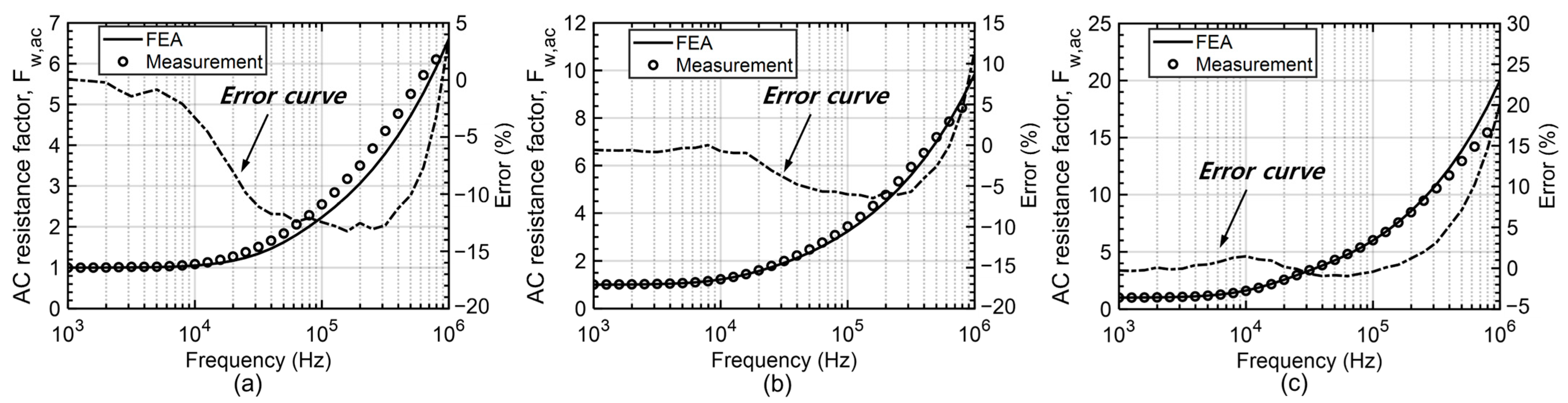
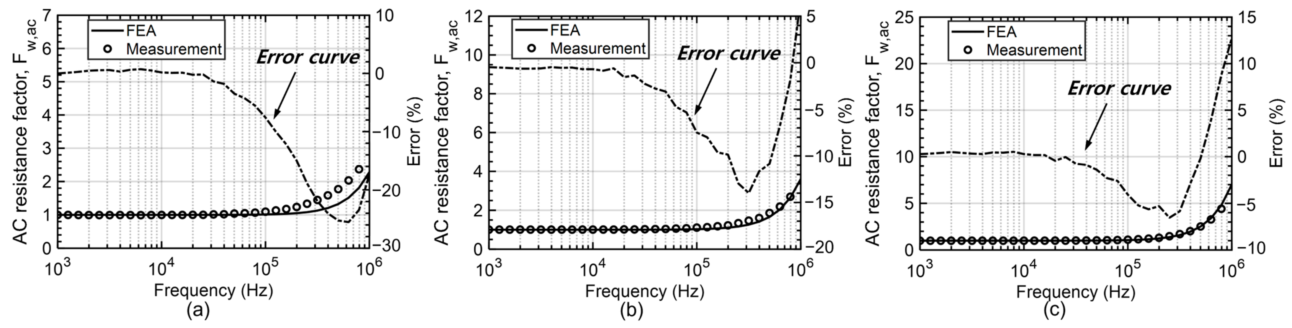
5.2. Experimental Results

The calculated results are compared with the resistance measurement to discuss the validity of the calculation. To measure the winding resistance, the resistance increments due to the core loss and parasitic capacitance pose the challenge of extracting the exact winding resistance [23]. In Section 2, the effect of the magnetic core can be negligible to the windings with high filling factors such as Inductor #3, #4, and #5. Although the magnetic core can change the magnetic field for the windings with lower filling factors (Inductors #1 and #2), the proximity effect is not dominant compared to the skin effect, so this study employs manufactured air-core toroidal windings, which can neglect the core loss and the parasitic capacitance within frequencies up to 1 MHz.
For the validation, Inductors #2, #3, and #5 were manufactured with both Litz wire and solid round wire, as presented in Figure 16. The resistance of the inductors was measured using an LCR meter (HIOKI IM 3536) which can measure the impedance to up to 8 MHz within accuracies of 0.05% for the magnitude and 0.03% for the phase measurement. Initially, the DC resistance was measured using a DC resistance meter (Bk Precision 2841), and the AC resistance was measured from 1 kHz to 1 MHz. Subsequently, the AC-resistance factors are calculated and compared with the FEA results.
The measured resistance of Inductor #2 as shown in Figure 17a and Figure 18a exhibit the relatively high error compared to those of Inductors #3 and #5. These deviations can originate from neglecting the magnetic core in this experiment. The existence of the magnetic core can increase the proximity effect compared to the air-core. Nevertheless, the error is below 15%, since the skin effect is more significant for the loosely wound core. The calculated resistance (FEA) of densely wound inductors (Inductors #3 and #5) shows good agreement, compared to the measured resistance, but the resistance of Inductor #5 addresses the increasing discrepancy, reaching 1 MHz due to the increment from the self-resonance. The good agreement between FEA and the measurement can provide promising results obtained from the proposed approach for both solid-round and Litz-wire windings (within 20% error across the wide spectrum of frequencies within 1 MHz in Table 3).

6. Conclusions

In this paper, the methodology for calculating the AC resistance is proposed for the solid-round and Litz-wire toroidal windings. While the modified Dowell’s method presents a promising option for inductor designers due to its simplicity and improved accuracy, it may overestimate the winding resistance in cases where the wires are not densely wound around the core. To address this limitation, the alternative approach based on the complex permeability is introduced. By generalizing the expression of the AC resistance for both solid and Litz-wire windings from the homogenization technique, the iterative approach is proposed to overcome the inaccurate calculation of most analytical methods.
The calculation results demonstrate good agreement with FEA, with deviation below 15%. In our future work, this work will be incorporated with the parasitic capacitance estimation, which makes the self-resonance characteristic and deviates the equivalent resistance of the inductor from a solitary consideration of the AC-winding resistance at higher frequencies. Additionally, the frequency approach in this article will be extended into the time domain to address the transient behavior of the inductor coupled with the power converters. Finally, this approach has a strong potential to be employed to more diverse applications, such as the slot geometry of the electric machines for analyzing the AC-winding loss at high speed [25]. Furthermore, this complex-permeability approach can be extended to the different shape of wires, specifically for the hairpin winding [26], and be evaluated for the contribution of the PWM excitation to the AC-winding loss, which will be covered in the author’s future works.

Author Contributions

Conceptualization, D.-Y.U. and G.-S.P.; methodology, D.-Y.U.; software, D.-Y.U.; investigation, D.-Y.U.; resources, D.-Y.U. and S.-A.C.; data curation, S.-A.C.; writing—original draft preparation, D.-Y.U.; writing—review and editing, G.-S.P.; visualization, D.-Y.U.; supervision, D.-Y.U.; project administration, D.-Y.U. and G.-S.P.; funding acquisition, G.-S.P. All authors have read and agreed to the published version of the manuscript.

Funding

This research was supported by Basic Science Research Program through the National Research Foundation of Korea (NRF) funded by the Ministry of Education (2020R1I1A3072753).

Data Availability Statement

The data used in this study are available from the corresponding author on reasonable request.

Conflicts of Interest

The authors declare no conflicts of interest.

References

  1. Iannaccone, G.; Sbrana, C.; Morelli, I.; Strangio, S. Power Electronics Based on Wide-Bandgap Semiconductors: Opportunities and Challenges. IEEE Access 2021, 9, 139446–139456. [Google Scholar] [CrossRef]
  2. Morya, A.K.; Gardner, M.C.; Anvari, B.; Liu, L.; Yepes, A.G.; Doval-Gandoy, J.; Toliyat, H.A. Wide Bandgap Devices in AC Electric Drives: Opportunities and Challenges. IEEE Trans. Transp. Electrif. 2019, 5, 3–20. [Google Scholar] [CrossRef]
  3. Kumar, A.; Moradpour, M.; Losito, M.; Franke, W.-T.; Ramasamy, S.; Baccoli, R.; Gatto, G. Wide Band Gap Devices and Their Application in Power Electronics. Energies 2022, 15, 9172. [Google Scholar] [CrossRef]
  4. Spang, M.; Albach, M. Optimized Winding Layout for Minimized Proximity Losses in Coils with Rod Cores. IEEE Trans. Magn. 2008, 44, 1815–1821. [Google Scholar] [CrossRef]
  5. Nan, X.; Sullivan, C.R. An Equivalent Complex Permeability Model for Litz-Wire Windings. IEEE Trans. Ind. Appl. 2009, 45, 854–860. [Google Scholar] [CrossRef]
  6. Gyselinck, J.; Dular, P. Frequency-domain homogenization of bundles of wires in 2-D magnetodynamic FE calculations. IEEE Trans. Magn. 2005, 41, 1416–1419. [Google Scholar] [CrossRef]
  7. Niyomsatian, K.; Gyselinck, J.; Sabariego, R.V. New closed-form proximity-effect complex permeability expression for characterizing litz-wire windings. In Proceedings of the Tenth International Conference on Computational Electromagnetics (CEM), Edinburgh, UK, 19–20 June 2019; pp. 1–2. [Google Scholar]
  8. Igarashi, H. Semi-Analytical Approach for Finite-Element Analysis of Multi-Turn Coil Considering Skin and Proximity Effects. IEEE Trans. Magn. 2017, 53, 1–7. [Google Scholar] [CrossRef]
  9. Otomo, Y.; Igarashi, H.; Sano, H.; Yamada, T. Analysis of Litz Wire Losses Using Homogenization-Based FEM. IEEE Trans. Magn. 2021, 57, 7402409. [Google Scholar] [CrossRef]
  10. Podoltsev, A.D.; Abeywickrama, K.G.N.B.; Serdyuk, Y.V.; Gubanski, S.M. Multiscale Computations of Parameters of Power Transformer Windings at High Frequencies. Part I: Small-Scale Level. IEEE Trans. Magn. 2007, 43, 3991–3998. [Google Scholar] [CrossRef]
  11. Etemadrezaei, M.; Lukic, S.M. Coated-Strand Litz Wire for Multi-Megahertz Frequency Applications. IEEE Trans. Magn. 2016, 52, 6301511. [Google Scholar] [CrossRef]
  12. Roßkopf, A.; Bär, E.; Joffe, C.; Bonse, C. Calculation of Power Losses in Litz Wire Systems by Coupling FEM and PEEC Method. IEEE Trans. Power Electron. 2016, 31, 6442–6449. [Google Scholar] [CrossRef]
  13. Taran, N.; Ionel, D.M.; Rallabandi, V.; Heins, G.; Patterson, D. An Overview of Methods and a New Three-Dimensional FEA and Analytical Hybrid Technique for Calculating AC Winding Losses in PM Machines. IEEE Trans. Ind. Appl. 2021, 57, 352–362. [Google Scholar] [CrossRef]
  14. Volpe, G.; Popescu, M.; Marignetti, F.; Goss, J. AC Winding Losses in Automotive Traction E-Machines: A New Hybrid Calculation Method. In Proceedings of the IEEE International Electric Machines & Drives Conference (IEMDC), San Diego, CA, USA, 12–15 May 2019; pp. 2115–2119. [Google Scholar]
  15. Acero, J.; Alonso, R.; Burdio, J.M.; Barragan, L.A.; Puyal, D. Frequency-dependent resistance in Litz-wire planar windings for domestic induction heating appliances. IEEE Trans. Power Electron. 2016, 21, 856–866. [Google Scholar] [CrossRef]
  16. Jabłoński, P.; Szczegielniak, T.; Kusiak, D.; Piątek, Z. Analytical–Numerical Solution for the Skin and Proximity Effects in Two Parallel Round Conductors. Energies 2019, 12, 3584. [Google Scholar] [CrossRef]
  17. Acero, J.; Alonso, R.; Barragan, L.A.; Burdio, J.M. Magnetic vector potential based model for eddy-current loss calculation in round-wire planar windings. IEEE Trans. Magn. 2006, 42, 2152–2158. [Google Scholar] [CrossRef]
  18. Cheng, K.W.E. Computation of the AC resistance of multistranded conductor inductors with multilayers for high frequency switching converters. IEEE Trans. Magn. 2000, 36, 831–834. [Google Scholar] [CrossRef]
  19. Geng, S.; Chu, M.; Wang, W.; Wan, P.; Peng, X.; Lu, H.; Li, P. Modelling and optimization of winding resistance for litz wire inductors. IET Power Electron. 2021, 14, 1834–1843. [Google Scholar] [CrossRef]
  20. Zhao, Y.; Ming, Z.; Han, B. Analytical modelling of high-frequency losses in toroidal inductors. IET Power Electron. 2023, 16, 1538–1547. [Google Scholar] [CrossRef]
  21. Elizondo, D.; Barrios, E.L.; Ursúa, A.; Sanchis, P. Analytical Modeling of High-Frequency Winding Loss in Round-Wire Toroidal Inductors. IEEE Trans. Power Electron. 2023, 70, 5581–5591. [Google Scholar] [CrossRef]
  22. Um, Y.; Park, G.S. Modeling of Frequency-Dependent Winding Losses in Solid and Litz-wire Toroidal Inductors. In Proceedings of the 25th International Conference on Electrical Machines and Systems (ICEMS), Chiang Mai, Thailand, 29 November–1 December 2022; pp. 1–6. [Google Scholar]
  23. Foo, B.X.; Stein, A.L.F.; Sullivan, C.R. A step-by-step guide to extracting winding resistance from an impedance measurement. In Proceedings of the IEEE Applied Power Electronics Conference and Exposition (APEC), Tampa, FL, USA, 26–30 March 2017; pp. 861–867. [Google Scholar]
  24. Um, D.Y.; Park, G.S. Resistance Variations in High-Frequency Inductors Considering Induced Fields Among Conductors. IEEE Trans. Magn. 2021, 57, 8400105. [Google Scholar] [CrossRef]
  25. Du, G.; Ye, W.; Zhang, Y.; Wang, L.; Pu, T. Comprehensive Analysis of Influencing Factors of AC Copper Loss for High-Speed Permanent Magnet Machine with Round Copper Wire Windings. Machines 2022, 10, 731. [Google Scholar] [CrossRef]
  26. Selema, A.; Ibrahim, M.N.; Sergeant, P. Mitigation of High-Frequency Eddy Current Losses in Hairpin Winding Machines. Machines 2022, 10, 328. [Google Scholar] [CrossRef]
Figure 1. A 3-D toroidal inductor and a simplified 2-D model represented by a cutting plane.
Machines 12 00228 g001
Figure 2. Comparison of the AC-winding loss factor calculated by the modified Dowell model and FEA for single-layer ((a) Inductor #2, (b) Inductor #3) and (c) double-layer (Inductor #5)-winding configurations.
Machines 12 00228 g002
Figure 3. The magnetic field distribution of (a) Inductor #1, (b) Inductor #2, (c) Inductor #4, and (d) Inductor #5.
Machines 12 00228 g003
Figure 4. FE simulation results of the azimuthal direction of magnetic fields in (a) Inductor #1, (b) Inductor #2, (c) Inductor #3, and (d) Inductor #4.
Machines 12 00228 g004
Figure 5. The composition of the AC-resistance factor for (a) Inductor #1, (b) Inductor #2, (c) Inductor #4, and (d) Inductor #5.
Machines 12 00228 g005
Figure 6. (a) The round wire immersed in the magnetic field, and (b) the eddy current behavior on a conductive medium and equivalent complex permeability to diamagnetism.
Machines 12 00228 g006
Figure 7. The complex permeability of a round wire calculated in Equation (8).
Machines 12 00228 g007
Figure 8. Homogenization of multiple strands by means of the complex permeability of a unit cell.
Machines 12 00228 g008
Figure 9. The simulation conditions to analyze the effect of a nearby wire on the proximity effect.
Machines 12 00228 g009
Figure 10. The calculated flux line in the cell region depicted in Figure 9 for (a) a single wire and (b) two wires at 100 kHz. The magnetic field intensity, 0.05 mm above the top of the wire along a line from point a to b in depicted in Figure 9 at (c) 100 kHz and (d) 1 MHz.
Machines 12 00228 g010
Figure 11. (a) Eddy current losses normalized by the loss calculated using FEA and analytical calculations based on a single wire at different frequencies and (b) the calculation error.
Machines 12 00228 g011
Figure 12. The concept of the iterative approach from the initial step to the next step.
Machines 12 00228 g012
Figure 13. (a) Eddy current losses normalized by the loss calculated using FEA, analytical calculation without any iteration (single calculation), and with the iterative method at different frequencies, and (b) the comparison of the error between with and without the iterative approach.
Machines 12 00228 g013
Figure 14. Comparison of the AC-winding loss factor calculated by the proposed model and FEA for single-layer ((a) Inductor #2, (b) Inductor #3) and (c) double-layer (Inductor #5) winding configurations, comprising solid round wires.
Machines 12 00228 g014
Figure 15. Comparison of the AC-winding loss factor calculated by the proposed model and FEA for single-layer ((a) Inductor #2, (b) Inductor #3) and (c) double-layer (Inductor #5) winding configurations, comprising Litz wires.
Machines 12 00228 g015
Figure 16. The manufactured inductors with air-core windings to measure the winding resistance.
Machines 12 00228 g016
Figure 17. Comparison of the AC-winding loss factor calculated by FEA and the measurement for single-layer ((a) Inductor #2, (b) Inductor #3) and (c) double-layer (Inductor #5) winding configurations, comprising solid round wires.
Machines 12 00228 g017
Figure 18. Comparison of the AC-winding loss factor calculated by FEA and the measurement for single-layer ((a) Inductor #2, (b) Inductor #3) and (c) double-layer (Inductor #5) winding configurations, comprising Litz wires.
Machines 12 00228 g018
Table 1. Winding structure and calculated results in the different five inductors (ANA: modified Dowell’s model, Inductor #5: turns and packing factor are expressed by first layer/second layer).
ModelLayerTurnsPacking FactorFw,ac @ 100 kHzFw,ac @ 1 MHzError
Inner SectionOuter SectionFEAANAFEAANA100 kHz1 MHz
Inductor #1150.1350.0692.101.846.126.13−12.38%0.16%
Inductor #21100.2700.1392.232.726.618.6721.97%31.16%
Inductor #31200.5400.2783.243.889.8412.2719.75%24.70%
Inductor #41250.6750.3473.874.3411.8513.7212.14%15.78%
Inductor #5220/100.540/0.3530.278/0.1246.006.4119.9819.836.83%−0.75%
Table 2. Comparison between FEA and calculated AC-resistance factor for five inductors at 100 kHz and 1 MHz.
ModelWire TypeFw,ac @ 100 kHzFw,ac @ 1 MHzErrorError
FEAProposedFEAProposed100 kHz1 MHz
Inductor #1Solid2.102.086.126.121.05%2.00%
Litz1.011.012.172.130.04%1.62%
Inductor #2Solid2.232.296.616.75−2.78%−2.19%
Litz1.011.012.282.30−0.02%−0.80%
Inductor #3Solid3.243.159.849.772.80%0.76%
Litz1.031.023.602.980.61%17.30%
Inductor #4Solid3.873.7911.8512.032.22%−1.57%
Litz1.031.034.113.490.61%15.15%
Inductor #5Solid6.006.9219.9823.15−15.45%−15.83%
Litz1.061.057.015.980.99%14.78%
Table 3. Comparison of AC-resistance factors obtained from the proposed calculation and measurement.
ModelWire TypeFw,ac @ 100 kHzFw,ac @ 1 MHzErrorError
ProposedMeasuredProposedMeasured100 kHz1 MHz
Inductor #2Solid2.292.556.616.37−10.20%3.77%
Litz1.011.12.282.76−8.18%−17.39%
Inductor #3Solid3.153.449.848.83−8.43%11.44%
Litz1.021.113.603.37−8.11%6.82%
Inductor #5Solid6.926.0219.9816.6514.95%20.00%
Litz1.051.117.016.22−5.41%12.70%
Disclaimer/Publisher’s Note: The statements, opinions and data contained in all publications are solely those of the individual author(s) and contributor(s) and not of MDPI and/or the editor(s). MDPI and/or the editor(s) disclaim responsibility for any injury to people or property resulting from any ideas, methods, instructions or products referred to in the content.

