Design of a Flexure-Based Flywheel for the Storage of Angular Momentum and Kinetic Energy

Abstract

The flywheel is a widespread mechanical component used for the storage of kinetic energy and angular momentum. It typically consists of cylindrical inertia rotating about its axis on rolling bearings, which involves undesired friction, lubrication, and wear. This paper presents an alternative mechanism that is functionally equivalent to a classical flywheel while relying exclusively on limited-stroke flexure joints. This novel one-degree-of-freedom zero-force mechanism has no wear and requires no lubrication: it is thus compatible with extreme environments, such as vacuum, cryogenics, or ionizing radiation. The mechanism is composed of two coupled pivoting rigid bodies whose individual angular momenta vary during motion but whose sum is constant at all times when the pivoting rate is constant. The quantitative comparison of the flexure-based flywheel to classical ones based on a hollow cylinder as inertia shows that the former typically stores 6 times less angular momentum and kinetic energy for the same mass while typically occupying 10 times more volume. The freedom of design of the shape of the rigid bodies offers the possibility of modifying the ratio of the stored kinetic energy versus angular momentum, which is not possible with classical flywheels. For example, a flexure-based flywheel with rigid pivoting bodies in the shape of thin discs stores 100 times more kinetic energy than a classical flywheel with the same angular momentum. A proof-of-concept prototype was successfully built and characterized in terms of reaction moment generation, which validates the presented analytical model.

1. Introduction

1.1. Flywheel State-of-the-Art and Article Contributions

Flywheels are mechanical components that are able to store kinetic energy (in the form of rotational energy) as well as angular momentum. We define a standard flywheel as a rigid body that rotates around an axis that coincides with its center of mass (COM) and is parallel to one of its principal axes of inertia. Flywheels have many applications, such as smoothing power output, serving as an additional source of energy, and generating reaction torques. The smoothing of power output is commonly found in reciprocating engines. Flywheels may serve in kinetic energy recovery system (KERS) applications to store and release kinetic energy harvested from the braking of a vehicle. They can be used as additional auxiliary power sources in the form of intermittent pulses (for a forging hammer, for example) or as a single impulse (for powering up a tokamak or aircraft catapult, for example). The generation of reaction torques comes from the flywheel’s ability to store angular momentum and finds its use in attitude control systems, such as the reaction wheels and control moment gyros of spacecrafts.

A standard flywheel is fixed to its base by means of a rotating bearing, such as ball bearings, gas bearings, or magnetic bearings, which permits multiple complete revolutions. Even though the flywheel is a well-established technology, the use of ball bearings may present drawbacks such as the need for lubrication and associated maintenance, as well as vacuum compatibility (lubricant outgassing and the hermeticity of the casing), if one wants to reduce air resistance as the flywheel rotates [1]. Gas bearings do not need any lubrication, but extra efforts should be made to encapsulate them to make them vacuum-compatible [2]. Finally, magnetic bearings solve all the presented issues at the cost of increased control complexity of the flywheel and higher consumption [3].

All the aforementioned bearing drawbacks can be addressed with the use of flexure-based bearings. Indeed, flexures work by using the elastic deformation of flexible members, thus eliminating friction, wear, and the need for lubrication while being vacuum-compatible and offering the possibility of miniaturization [4]. The only property that intuitively prevents flexures from being used as the flywheel’s bearing is the multiple complete revolutions the latter must achieve.

This article proposes an alternative design of a flywheel, first introduced in [5], that is compatible with the use of flexures in the sense that this mechanism can store kinetic energy and generate angular momentum and has limited stroke at each joint. In addition, a comparative study of performances is drawn between a standard flywheel and the proposed flexure design.

1.2. Requirements for a Flexure-Based Flywheel Equivalent

To establish criteria for a flexure-based flywheel equivalent, the key properties of a standard flywheel need to be highlighted. First, the flywheel’s center of mass remains fixed during its motion and therefore does not export any forces during motion. This property is defined by Schneegans et al. as being force-balanced [6]. The flywheel is also in equilibrium when at rest (i.e., is not subject to any forces), regardless of its orientation, and therefore has constant potential energy, a property defined as statically balanced by [6]. During its motion, the flywheel generates angular momentum that is constant in amplitude and in direction. Last, if the standard flywheel has a cylindrical shape, as in most cases, the inertia tensor of the flywheel, as seen from its base, does not change. If this is not the case and if the flywheel’s base is also rotating, the flywheel will export torque. This last property, defined as inertial invariance by [6], is, however, regarded as optional as its effect will only be apparent for a flywheel whose base is rotating.

To allow the selection of an appropriate design, the properties described above are now enumerated:

• The center of mass of the reaction mechanism must remain fixed throughout its motion.
• The mechanism must be able to generate angular momentum that is constant in direction.
• The mechanism must be able to generate angular momentum that is constant in amplitude.
• The mechanism must be able to control the amplitude of its angular momentum in order to deliver a reaction torque.
• The inertia tensor of the flywheel, as seen from its base, must remain constant throughout the motion (optional).

1.3. Outline of Paper

Section 2.1 defines the inertial bodies considered in this paper, along with the definition of constant velocity joints (CV joints) and their notational conventions. The flexure-based flywheel and its working principle will then be presented with ideal joints in Section 2.2. Even though this flywheel uses ideal joints (and therefore not necessarily flexures), it will still be referred to as a flexure-based flywheel to avoid additional terminology. In Section 2.3.2, the kinetic energy and angular momentum of this mechanism will be discussed, followed by the internal forces that transit through the joints (Section 2.4). In Section 3, a comparative study between a standard flywheel and the flexure-based design will then be shown, and their performances in terms of kinetic energy, angular momentum, and volume will be discussed. Section 4 shows the influence of the shape ratio of pivoting cylindrical rigid bodies on the generation of angular momentum and storage of kinetic energy. Thereafter, we highlight in Section 5 the analogy between the proposed mechanism and a falling cat. Last, in Section 6, an example of a flexure implementation, along with the constructed proof-of-concept prototype and experimental measurements, will be shown.

2. Flexure-Based Flywheel

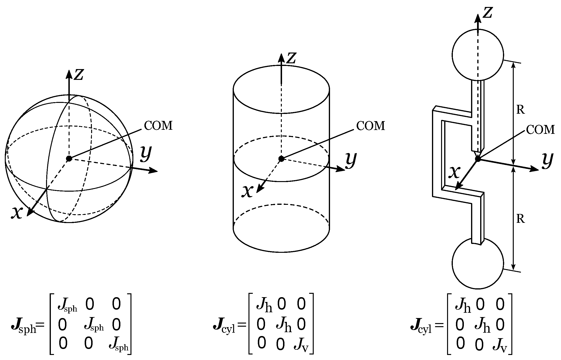
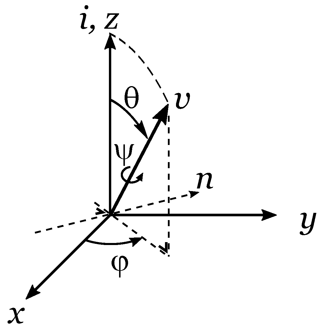
2.1. Definition of Specific Inertial Bodies and CV-Joint Kinematics

Before presenting the mechanism and its working principle, the types of inertial bodies present in this paper are introduced, along with the notion of CV joints and the notational conventions used to describe their kinematics.

We define a spherical inertial body as a rigid body in which all three moments of inertia around its principal axes of inertia are identical. Its inertia tensor ${\mathit{J}}_{\mathrm{sph}}$, when evaluated in the frame of its principle axes of inertia is given by:

$$\begin{array}{cc}\hfill {\mathit{J}}_{\mathrm{sph}}& =\left[\begin{array}{ccc}{J}_{\mathrm{sph}}& 0& 0\\ 0& J_{\mathrm{sph}}& 0\\ 0& 0& J_{\mathrm{sph}}\end{array}\right]\hfill \end{array}$$

(1)

We define a cylindrical inertial body as a rigid body in which two moments of inertia around its principle axes of inertia are identical, and it is assumed that these two principle axes coincide with the x- and y-axes. Its inertia tensor ${\mathit{J}}_{\mathrm{cyl}}$, when evaluated in the frame of its principal axes of inertia, is given by the following ($J_{\mathrm{h}}$ and $J_{\mathrm{v}}$ have been chosen as the notation to designate the moments of inertia around the ’horizontal’ axes x and y and moment of inertia around the ’vertical’ z-axis):

$$\begin{array}{cc}\hfill {\mathit{J}}_{\mathrm{cyl}}& =\left[\begin{array}{ccc}{J}_{\mathrm{h}}& 0& 0\\ 0& J_{\mathrm{h}}& 0\\ 0& 0& J_{\mathrm{v}}\end{array}\right]\hfill \end{array}$$

(2)

A cylindrical inertial body is not necessarily a cylinder but can take other shapes. A dumbbell is another embodiment of a cylindrical inertial body as it results in the same inertia tensor, as shown in Figure 1 (right).

The orientation of rigid bodies will be described using Euler angles. The convention for the three successive rotations is depicted in Figure 2, in which the body is first rotated around the z-axis by angle $\phi$ (azimuth), then rotated around $\mathit{n}$ by angle $\theta$ (elevation), and finally around axis $\mathit{v}$ by angle $\psi$ (twist). Moreover, the notational convention we adopt for the rotation matrix describing a rotation $\alpha$ around an axis $\mathit{a}$ is ${\mathit{R}}_{\mathit{a}}\left(\alpha \right)$. The rotation of a body is therefore given by the product ${\mathit{R}}_{\mathit{z}}\left(\phi \right){\mathit{R}}_{\mathit{y}}\left(\theta \right){\mathit{R}}_{\mathit{z}}\left(\psi \right)$.

CV joints are variants of the universal joint and are typically used for the transmission of torque from one rotating shaft to another without any variation in speed. In this paper, these same CV joints are in a different configuration, in which the input shaft is fixed and the output shaft has two rotational degrees of freedom. The kinematics of a CV joint in terms of Euler angles have been described by Vardi et al. [7], who states that the joint has zero torsion (i.e., $\psi =-\phi$). Indeed, the $\phi$ rotation around $\mathbf{i}$-axis counterintuitively introduces a torsion component that needs to be retrieved from the twist parameter $\psi$. This means that the kinematics of a CV-joint are given by the product rotation matrix ${\mathit{R}}_{\mathrm{CV}}(\theta ,\phi )$:

$${\mathit{R}}_{\mathrm{CV}}(\theta ,\phi )={\mathit{R}}_{\mathit{z}}\left(\phi \right){\mathit{R}}_{\mathit{y}}\left(\theta \right){\mathit{R}}_{\mathit{z}}(-\phi )$$

(3)

in which

$${\mathit{R}}_{\mathit{z}}(-\phi )=\left[\begin{array}{ccc}cos\phi & sin\phi & 0\\ -sin\phi & cos\phi & 0\\ 0& 0& 1\end{array}\right];{\mathit{R}}_{\mathit{y}}\left(\theta \right)=\left[\begin{array}{ccc}cos\theta & 0& sin\theta \\ 0& 1& 0\\ -sin\theta & 0& cos\theta \end{array}\right];{\mathit{R}}_{\mathit{z}}\left(\phi \right)=\left[\begin{array}{ccc}cos\phi & -sin\phi & 0\\ sin\phi & cos\phi & 0\\ 0& 0& 1\end{array}\right]$$

(4)

2.2. Description of the Mechanism and Working Principle

As shown in Figure 3, the mechanism is composed of two identical cylindrical rigid bodies (1) and (2), which are each attached to a fixed base (3) via CV-joints (A), respectively (B), located at each body’s center of mass. Bodies (1) and (2) are connected with one another via a ball joint (C) located equidistant from (A) and (B) (i.e., the distances are, e.g., $AC=BC$ and $AC+BC>AB$). This arrangement forces the center of the ball joint (C) to remain at a constant distance from the $AB$ line. As a result, when the mechanism moves, (C) follows a circular path, the elevation angles of the two CV joints are equal and constant (${\theta }_1={\theta }_2$), and the azimuth angles of the two CV joints have a phase shift of $\pi$ (${\phi }_1={\phi }_2+\pi$). This motion, which keeps a fixed elevation and sweeps the azimuth, shall be defined as the pivoting motion.

The working principle at play is that the angular momenta of each pivoting body are oblique. When the whole mechanism is considered, the x and y components of the angular momentum are canceled out, and only the constant z component remains. This one-degree-of-freedom mechanism is isostatic (also called statically determinate or proper constraint), meaning that it is neither under-constraint (i.e., with internal degrees-of-freedom) nor over-constraint (i.e., with kinematic chains that block several times the same degrees of freedom). Also, when it moves, this mechanism presents the following key properties:

• One degree of freedom, i.e., the azimuth angle $\phi$ fully determines the position of both segments (1) and (2).
• For a constant velocity, $\dot{\phi }=\mathrm{constant}$, the total angular momentum of the mechanism is constant.
• The angular deflection of the two CV joints (A) and (B) in elevation remains constant at all times $\theta =\mathrm{constant}$.
• The angular deflection of the ball joint (C) in elevation $\rho$ remains constant at all times and equal to $\rho =2\theta =\mathrm{constant}$.
• If the joints (A), (B), and (C) have positive isotropic (in the sense that the stiffness does not vary with $\phi$, i.e., that the stiffness is the same for all tilting directions) angular stiffnesses, then the elastic potential energy of the mechanism remains constant at all times and the mechanism is statically balanced (i.e., the mechanism as a whole is zero force and is stable in any position). The total elastic potential energy of the mechanism may vary with $\phi$ if the flexure joints exhibit stiffness anisotropy. In this case, the actuation of the mechanism may be disturbed by one or multiple stable states.
• If the rigid bodies (1) and (2) are also spherical rigid bodies, then the inertia tensor of the mechanism as a whole remains constant at all times, and condition 5 is fulfilled.

2.3. Kinematics

2.3.1. Kinematics of Rigid Body 1

Let ${\mathcal{R}}_A$ be the inertial frame centered on (A) whose axes are parallel to the x-, y-, and z-axes.

In rigid body 1’s attached frame (coincident with its principal axes), rigid body 1’s inertia tensor ${\mathit{J}}_{\mathrm{cyl}}$ is given by Equation (2). Following Equation (3), the orientation of rigid body 1 is given by the rotation matrix ${\mathit{R}}_{\mathrm{CV},1}$:

$$\begin{array}{cc}\hfill {\mathit{R}}_{\mathrm{CV},1}& ={\mathit{R}}_{\mathrm{CV}}(\theta ,\phi )\hfill \end{array}$$

(5)

As seen in inertial frame ${\mathcal{R}}_A$, rigid body 1’s inertia tensor ${\mathit{J}}_{1,{\mathcal{R}}_{\mathrm{A}}}$ is given by

$$\begin{array}{cc}\hfill {\mathit{J}}_{1,{\mathcal{R}}_{\mathrm{A}}}& ={\mathit{R}}_{\mathrm{CV},1}{\mathit{J}}_{\mathrm{cyl}}{\mathit{R}}_{\mathrm{CV},1}^{⊺}.\hfill \end{array}$$

(6)

Vardi [7] also provides a formula for the angular velocity of the pivoting rigid body 1, evaluated in ${\mathcal{R}}_A$. Vardi explains that when Euler angles are used, the angular velocity $\mathit{\omega }$ is given by

$$\mathit{\omega }=\dot{\phi }\mathbf{i}+\dot{\theta }\mathbf{n}+\dot{\psi }\mathbf{v},$$

(7)

Considering $\dot{\theta }=0$, as the elevation angle of pivoting rigid body 1 is set as constant and $\dot{\psi }=-\dot{\phi }$ to have a zero-torsion CV-joint, the previous equation is simplified and becomes

$$\begin{array}{cc}\hfill {\mathit{\omega }}_1& =\dot{\phi }\left(\mathbf{i}-\mathbf{v}\right)=\dot{\phi }\left(\left[\begin{array}{c}0\\ 0\\ 1\end{array}\right]-{\mathit{R}}_{\mathrm{CV},1}\left[\begin{array}{c}0\\ 0\\ 1\end{array}\right]\right)=\dot{\phi }\left[\begin{array}{c}-cos\phi sin\theta \\ -sin\phi sin\theta \\ \left(1-cos\theta \right)\end{array}\right]\hfill \end{array}$$

(8)

The angular momentum ${\mathit{L}}_1$ of pivoting rigid body 1, evaluated in ${\mathcal{R}}_A$ is then given by

$$\begin{array}{cc}\hfill {\mathit{L}}_1& ={\mathit{J}}_{1,{\mathcal{R}}_{\mathrm{A}}}{\mathit{\omega }}_1=\dot{\phi }\left[\begin{array}{c}-cos\phi \left(\left(J_{\mathrm{h}}-J_{\mathrm{v}}\right)cos\theta +J_{\mathrm{v}}\right)sin\theta \\ -sin\phi \left(\left(J_{\mathrm{h}}-J_{\mathrm{v}}\right)cos\theta +J_{\mathrm{v}}\right)sin\theta \\ \left(1-cos\theta \right)\left(\left(J_{\mathrm{h}}-J_{\mathrm{v}}\right)cos\theta +J_{\mathrm{h}}\right)\end{array}\right]\hfill \end{array}$$

(9)

along with its kinetic energy $K_1$:

$$\begin{array}{cc}\hfill K_1& =\frac{1}{2}{\mathit{\omega }}_1^{⊺}{\mathit{J}}_{1,{\mathcal{R}}_{\mathrm{A}}}{\mathit{\omega }}_1=\frac{1}{2}{\dot{\phi }}^2\left(1-cos\theta \right)\left(\left(J_{\mathrm{h}}-J_{\mathrm{v}}\right)cos\theta +J_{\mathrm{v}}+J_{\mathrm{h}}\right).\hfill \end{array}$$

(10)

Observe from Equations (8) and (9) that ${\mathit{\omega }}_1$ and ${\mathit{L}}_1$ lie in the same vertical plane but are only colinear in the case of spherical inertia, i.e., when $J_h=J_v$. The same applies to ${\mathit{\omega }}_2$ and ${\mathit{L}}_2$.

2.3.2. Kinematics of Rigid Body 2

Similarly, as for rigid body 1, the rotation matrix ${\mathit{R}}_{\mathrm{CV},2}$ for rigid body 2 is given by

$$\begin{array}{cc}\hfill {\mathit{R}}_{\mathrm{CV},2}& ={\mathit{R}}_{\mathrm{CV}}(\theta ,\phi +\pi )\hfill \end{array}$$

(11)

Let ${\mathcal{R}}_B$ be the inertial frame centered on (B), whose axes are parallel to the x-, y-, and z-axes. Rigid body 2’s inertia tensor, as seen in inertial frame ${\mathcal{R}}_B$, is given by

$$\begin{array}{cc}\hfill {\mathit{J}}_{2,{\mathcal{R}}_{\mathrm{B}}}& ={\mathit{R}}_{\mathrm{CV},2}{\mathit{J}}_{\mathrm{cyl}}{\mathit{R}}_{\mathrm{CV},2}^{⊺}\hfill \end{array}$$

(12)

The angular velocity of the pivoting inertial body 2, evaluated in ${\mathcal{R}}_B$, is calculated in the same manner as inertial body 1:

$$\begin{array}{cc}\hfill {\mathit{\omega }}_2& =\dot{\phi }\left(\mathbf{i}-\mathbf{v}\right)=\dot{\phi }\left(\left[\begin{array}{c}0\\ 0\\ 1\end{array}\right]-{\mathit{R}}_{\mathrm{CV},2}\left[\begin{array}{c}0\\ 0\\ 1\end{array}\right]\right)=\dot{\phi }\left[\begin{array}{c}cos\phi sin\theta \\ sin\phi sin\theta \\ \left(1-cos\theta \right)\end{array}\right]\hfill \end{array}$$

(13)

The angular momentum ${\mathit{L}}_2$ of pivoting inertial body 2, evaluated in ${\mathcal{R}}_B$, is then given by:

$$\begin{array}{cc}\hfill {\mathit{L}}_2& ={\mathit{J}}_{2,{\mathcal{R}}_{\mathrm{B}}}{\mathit{\omega }}_2=\dot{\phi }\left[\begin{array}{c}cos\phi \left(\left(J_{\mathrm{h}}-J_{\mathrm{v}}\right)cos\theta +J_{\mathrm{v}}\right)sin\theta \\ sin\phi \left(\left(J_{\mathrm{h}}-J_{\mathrm{v}}\right)cos\theta +J_{\mathrm{v}}\right)sin\theta \\ \left(1-cos\theta \right)\left(\left(J_{\mathrm{h}}-J_{\mathrm{v}}\right)cos\theta +J_{\mathrm{h}}\right)\end{array}\right],\hfill \end{array}$$

(14)

whose z component is similar to the one of ${\mathit{L}}_1$. Likewise, its kinetic energy $K_2$ is:

$$\begin{array}{cc}\hfill K_2& =\frac{1}{2}{\mathit{\omega }}_2^{⊺}{\mathit{J}}_{2,{\mathcal{R}}_{\mathrm{B}}}{\mathit{\omega }}_2=\frac{1}{2}{\dot{\phi }}^2\left(1-cos\theta \right)\left(\left(J_{\mathrm{h}}-J_{\mathrm{v}}\right)cos\theta +J_{\mathrm{v}}+J_{\mathrm{h}}\right),\hfill \end{array}$$

(15)

which equals the kinetic energy $K_1$ of inertial body 1.

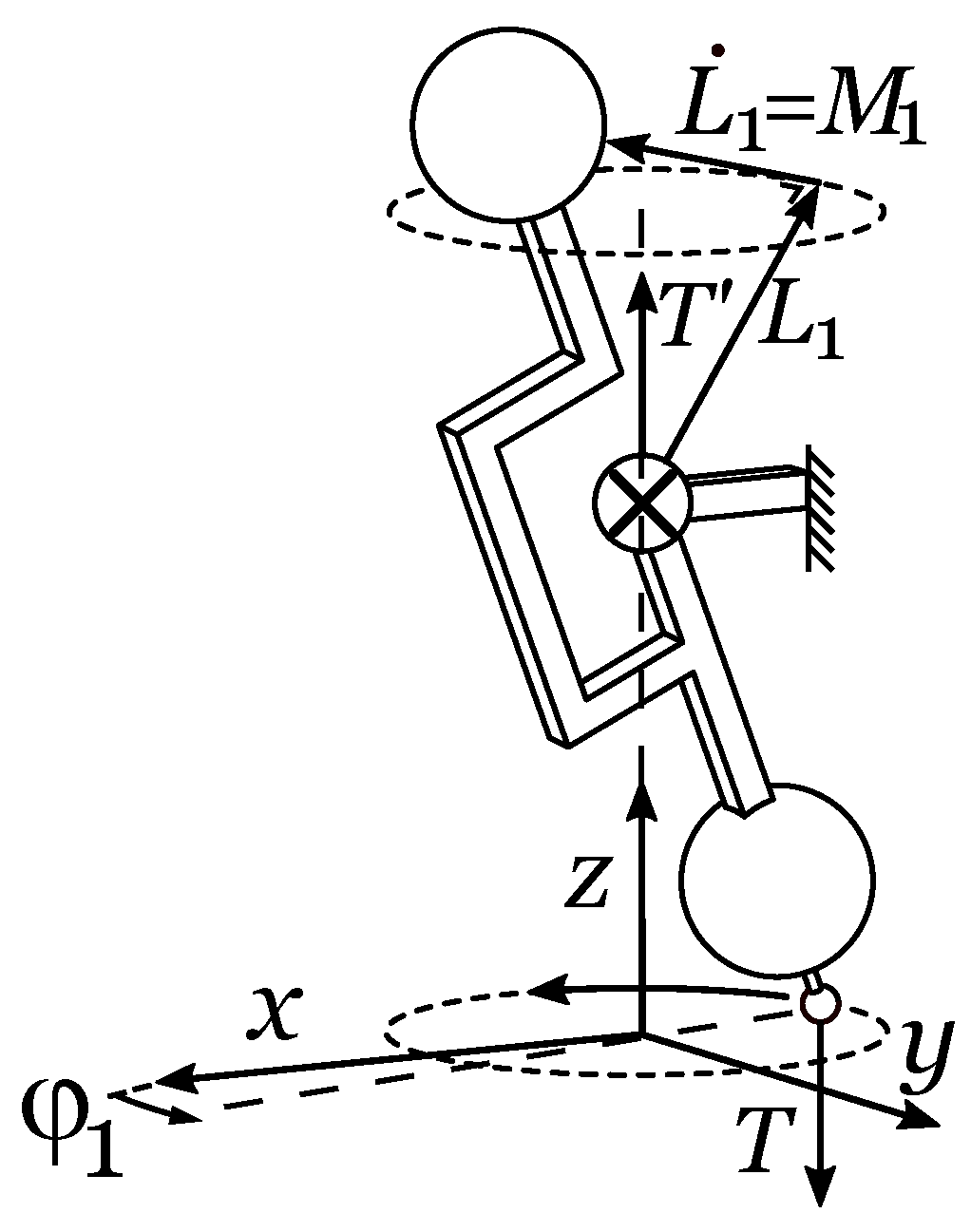
2.3.3. Angular Momentum and Kinetic Energy of the Complete Mechanism

As the centers of mass of rigid bodies 1 and 2 remain fixed during the pivoting motion, their angular momenta do not depend on which inertial frame is used. As for their kinetic energies, they are always independent of the considered inertial frame. For ease, we will evaluate the complete mechanism in the inertial frame ${\mathcal{R}}_0$ centered on O and whose axes coincide with the x-, y-, and z-axes. The complete mechanism’s angular momentum ${\mathit{L}}_{\mathrm{tot}}$, evaluated in ${\mathcal{R}}_0$, is then

$$\begin{array}{cc}\hfill {\mathit{L}}_{\mathrm{tot}}& ={\mathit{L}}_1+{\mathit{L}}_2=\dot{\phi }\left[\begin{array}{c}0\\ 0\\ 2\left(1-cos\theta \right)\left(\left(J_{\mathrm{h}}-J_{\mathrm{v}}\right)cos\theta +J_{\mathrm{h}}\right)\end{array}\right]\hfill \end{array}$$

(16)

It can be seen that in order to develop a maximum angular momentum, it is advantageous to increase the elevation $\theta$ and to opt for long and slender cylindrical bodies (as this increases $J_{\mathrm{h}}$ and decreases $J_{\mathrm{v}}$). From here, we can introduce $J_{\mathrm{equ},\mathrm{L}}$: the angular momentum equivalent moment of inertia, defined as follows:

$$\begin{array}{cc}\hfill J_{\mathrm{equ},\mathrm{L}}& =\frac{{\mathit{L}}_{\mathrm{tot}}}{\dot{\phi }}·\left[\begin{array}{c}0\\ 0\\ 1\end{array}\right]=2\left(1-cos\theta \right)\left(\left(J_{\mathrm{h}}-J_{\mathrm{v}}\right)cos\theta +J_{\mathrm{h}}\right).\hfill \end{array}$$

(17)

Note that the purpose of $J_{\mathrm{equ},\mathrm{L}}$ is to evaluate how much angular momentum is generated as a function of the pivoting rate $\dot{\phi }$. The kinetic energy $K_{\mathrm{tot}}$ of the complete mechanism is given by

$$\begin{array}{cc}\hfill K_{\mathrm{tot}}& =K_1+K_2={\dot{\phi }}^2\left(1-cos\theta \right)\left(\left(J_{\mathrm{h}}-J_{\mathrm{v}}\right)cos\theta +J_{\mathrm{v}}+J_{\mathrm{h}}\right).\hfill \end{array}$$

(18)

From this, we can introduce $J_{\mathrm{equ},\mathrm{K}}$: the kinetic energy equivalent moment of inertia, defined as follows:

$$\begin{array}{cc}\hfill J_{\mathrm{equ},\mathrm{K}}& =\frac{2K_{\mathrm{tot}}}{{\dot{\phi }}^2}=2\left(1-cos\theta \right)\left(\left(J_{\mathrm{h}}-J_{\mathrm{v}}\right)cos\theta +J_{\mathrm{v}}+J_{\mathrm{h}}\right).\hfill \end{array}$$

(19)

Note that the purpose of $J_{\mathrm{equ},\mathrm{K}}$ is to evaluate how much kinetic energy is generated as a function of the pivoting rate $\dot{\phi }$.

2.4. Joint Solicitation through Internal Forces

This section evaluates the internal forces that transit through the CV joints and ball joints in the stationary case (i.e., $\dot{\phi }$ is constant). The approach is to isolate one of the pivoting rigid bodies (rigid body 1 is chosen for this example) and to determine the net torque and force that are applied to it. The net torque applied to rigid body 1 is determined by calculating the time variation of its angular momentum ${\dot{\mathit{L}}}_1$:

$$\begin{array}{cc}\hfill {\dot{\mathit{L}}}_1& ={\dot{\phi }}^{2}sin\theta \left(\left({\mathit{J}}_{\mathrm{h}}-{\mathit{J}}_{\mathrm{v}}\right)cos\theta +{\mathit{J}}_{\mathrm{v}}\right)\left[\begin{array}{c}sin\phi \\ -cos\phi \\ 0\end{array}\right].\hfill \end{array}$$

(20)

This vector lies within the $xy$ plane, has a constant amplitude, and rotates at a fixed rate around the z-axis, as shown in Figure 4. Indeed, the net torque ${\mathit{M}}_1$ applied to rigid body 1 equals ${\dot{\mathit{L}}}_1$:

$${\mathit{M}}_1={\dot{\mathit{L}}}_1.$$

(21)

Concerning the net force applied to rigid body 1, since its center of mass remains fixed during motion, the applied net force is zero. Moreover, due to symmetry considerations, the internal force $\mathit{T}$ transiting through the ball joint, applied by rigid body 2 onto rigid body 1, is parallel to the z-axis. This means that the CV-joint applies a force ${\mathit{T}}^{\prime }=-\mathit{T}$, also parallel to the z-axis, onto rigid body 1 and that $\mathit{T}$ and ${\mathit{T}}^{\prime }$ form a couple together. As flexures are to be used in this flywheel, it can be assumed that the CV joints and ball joints have isotropic (in the sense that the stiffness does not vary with $\phi$, i.e., that the stiffness is the same for all tilting directions) angular stiffnesses $k_A$ and $k_C$, respectively. The net torque ${\mathit{M}}_1$ is given by

$$\begin{array}{cc}\hfill {\mathit{M}}_1& =\left(k_A\theta +k_C\left(2\theta \right)\right)\left[\begin{array}{c}sin\phi \\ -cos\phi \\ 0\end{array}\right]+\left[\begin{array}{c}-Rsin\theta cos\phi \\ -Rsin\theta sin\phi \\ -Rcos\theta \end{array}\right]\times \mathit{T}\hfill \\ \hfill & =\left(TRsin\theta +k_A\theta +k_C\left(2\theta \right)\right)\left[\begin{array}{c}sin\phi \\ -cos\phi \\ 0\end{array}\right],\hfill \end{array}$$

(22)

with T being the amplitude of force $\mathit{T}={\left[00-T\right]}^{⊺}$. From Equations (20)–(22), the amplitude T of force $\mathit{T}$ is given by

$$T=\frac{{\dot{\phi }}^{2}sin\theta \left(\left({\mathit{J}}_{\mathrm{h}}-{\mathit{J}}_{\mathrm{v}}\right)cos\theta +{\mathit{J}}_{\mathrm{v}}\right)-k_A\theta -k_C\left(2\theta \right)}{\mathit{R}sin\theta }.$$

(23)

An interesting property is that this force increases with ${\dot{\phi }}^2$, which resembles the behavior of a centripetal force. Another notable property of this formula is that the joints’ stiffnesses, which can be viewed as a preload, reduce the effective joint solicitation.

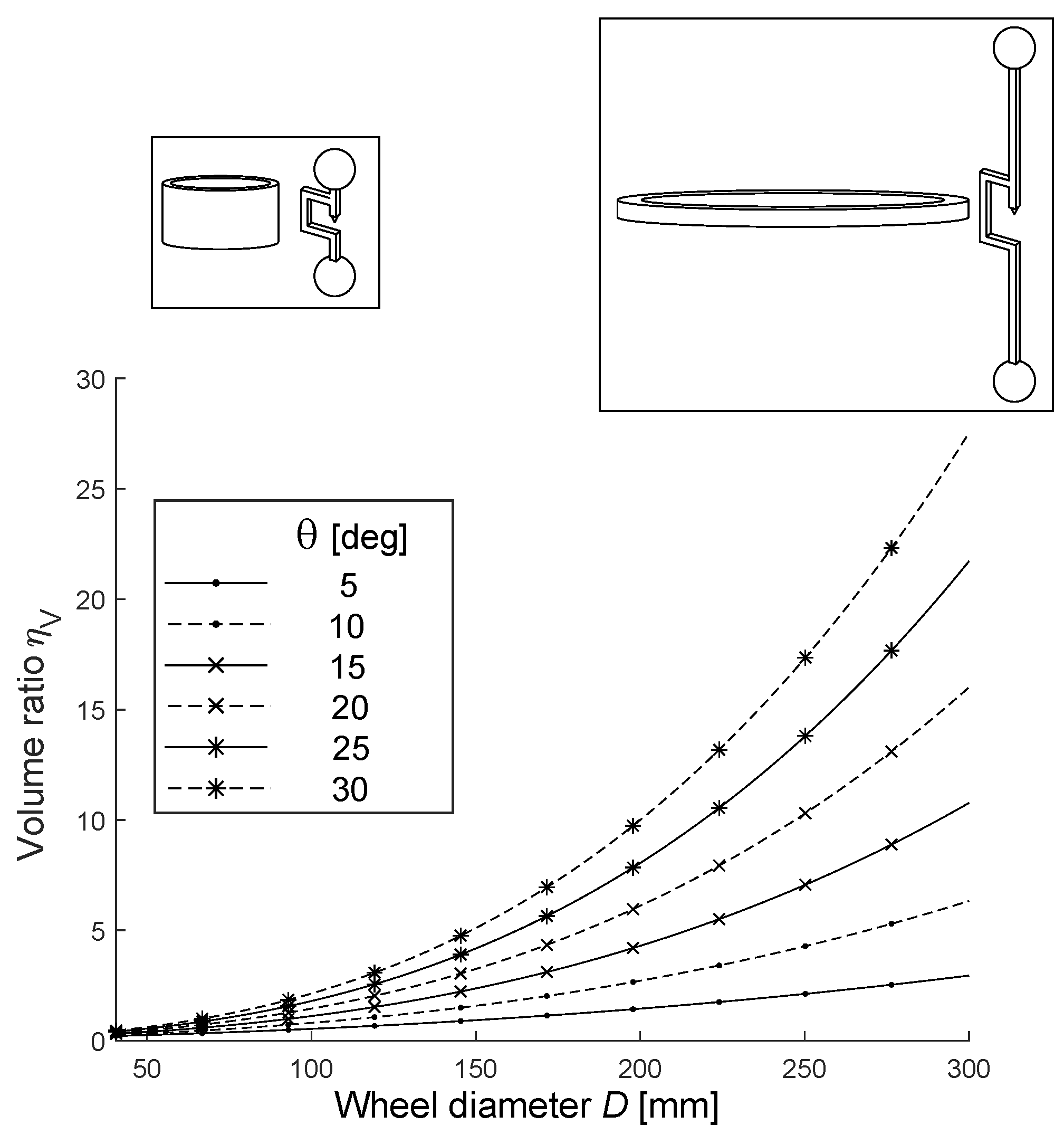
3. Comparison of a Dumbbell Flexure Design to a Standard Flywheel

This section compares the angular momentum and kinetic energy of the flexure-based flywheel to those of a standard flywheel. The standard flywheel selected as a benchmark for this comparison is a hollow cylinder, whose thickness-to-radius ratio $\xi$ is fixed to 0.1 (see Figure 5):

$$\xi =\frac{2w}{D}=\frac{1}{10}.$$

(24)

To allow a comparison to be drawn, both the flexure-based and standard designs have the same total mass M, and the dumbbell’s length $2R$ matches the flywheel’s diameter D, as shown in Figure 5.

The moment of inertia of the standard flywheel is given by

$$\begin{array}{cc}\hfill J_{\mathrm{std}}& =\frac{M{D}^2\left({\xi }^2-2\xi +2\right)}{8}.\hfill \end{array}$$

(25)

Moreover, in order to reach the correct mass M, this standard flywheel has a height H given by

$$H=\frac{4M}{\rho \pi D^2\xi \left(2-\xi \right)},$$

(26)

resulting in an envelope volume $V_{\mathrm{std}}$ given by

$$\begin{array}{cc}\hfill V_{\mathrm{std}}& =\pi {\left(\frac{D}{2}\right)}^{2}H=\frac{M}{\rho \xi \left(2-\xi \right)}.\hfill \end{array}$$

(27)

For the compared flexure design, the sphere-shaped masses m and their radii r are given by

$$\begin{array}{cc}\hfill m=& \frac{M}{4}\mathrm{and}r={\left(\frac{3m}{4\pi \rho }\right)}^{\frac{1}{3}},\hfill \end{array}$$

(28)

with $\rho$ the material’s density. This yields

$$\begin{array}{cc}\hfill J_{\mathrm{h}}& =2m·\left(\frac{2}{5}{r}^2+{\left(\frac{D}{2}\right)}^2\right)\mathrm{and}{J}_{\mathrm{v}}=\frac{4}{5}m{r}^2.\hfill \end{array}$$

(29)

Moreover, the cylindrical envelope of this dumbbell design, highlighted in Figure 5, has a volume V given by

$$\begin{array}{cc}\hfill V& =\pi {\left(\frac{D}{2}sin\theta +r\right)}^2\left(Dcos\theta +2r\right).\hfill \end{array}$$

(30)

The figures of merit of this comparison are ${\eta }_L$, ${\eta }_K$, and ${\eta }_V$, defined as

$${\eta }_L=\frac{J_{\mathrm{equ},\mathrm{L}}}{J_{\mathrm{std}}},{\eta }_K=\frac{J_{\mathrm{equ},\mathrm{K}}}{J_{\mathrm{std}}}\mathrm{and}{\eta }_V=\frac{V}{V_{\mathrm{std}}}.$$

(31)

These figures of merit describe the change in angular momentum, kinetic energy, and volume between a standard flywheel and the flexure-based flywheel. These are given by

$$\begin{array}{cc}\hfill {\eta }_L& =\frac{4\left(1-cos\theta \right)}{\left({\xi }^2-2\xi +2\right)}\left[\frac{1}{5D^2}{\left(\frac{6m}{\rho \pi }\right)}^{\frac{2}{3}}+\frac{\left(cos\theta +1\right)}{2}\right],\hfill \end{array}$$

(32)

$$\begin{array}{cc}\hfill {\eta }_K& =\frac{8\left(1-cos\theta \right)}{\left({\xi }^2-2\xi +2\right)}\left[\frac{1}{5D^2}{\left(\frac{6m}{\rho \pi }\right)}^{\frac{2}{3}}+\frac{\left(cos\theta +1\right)}{4}\right]\hfill \end{array}$$

(33)

and

$$\begin{array}{cc}\hfill {\eta }_V& =\frac{\rho \pi \xi \left(2-\xi \right)}{8m}{\left(Dsin\theta +{\left(\frac{6m}{\rho \pi }\right)}^{\frac{1}{3}}\right)}^2\left(Dcos\theta +{\left(\frac{6m}{\rho \pi }\right)}^{\frac{1}{3}}\right).\hfill \end{array}$$

(34)

The three figures of merit ${\eta }_L$, ${\eta }_K$, and ${\eta }_V$ are plotted in Figure 6, Figure 7 and Figure 8, for masses $m=0.1$ kg out of steel (density $\rho =8000$ kg/m³). Note that the range of D in these plots was selected to avoid interference of sphere-shaped masses within dumbbells, as this would not be realistic.

Equations (32) and (33) can be further simplified in the case of small masses m (or elongated dumbbells with large D). In this case, $\frac{m}{\rho }\simeq 0$, simplifying ${\eta }_L$ and ${\eta }_K$ to

$${\eta }_L\simeq {\eta }_K\simeq \frac{2{sin}^2\theta }{{\xi }^2-2\xi +2}.$$

(35)

It can indeed be seen in Figure 6 and Figure 7 that, with the exception of the smaller diameters, the diameter D has little influence on ${\eta }_L$ and ${\eta }_K$, as they depend mainly on $\theta$. The conclusions to draw from the first two graphs are that even though increasing the size of the flexure-based design increases the kinetic energy and angular momentum storage capacity, these keep the same proportion with respect to a standard flywheel. The only way to increase the storage capacity of this dumbbell design is to increase its tilt amplitude $\theta$. All curves remain below one, meaning angular momentum and kinetic energy are always lower than for the equivalent flywheel. For the typical range of $\theta ={20}^{\circ }$ for the deflection of flexures (as this results in a deflection of ${40}^{\circ }$ at the ball joint), the kinetic energy and angular momentum lose almost an order of magnitude. As for ${\eta }_L$ and ${\eta }_K$, the same simplification can be applied to ${\eta }_V$:

$${\eta }_V\simeq \frac{\pi {\mathit{D}}^3{sin}^2\theta cos\theta \rho \xi \left(2-\xi \right)}{16m},$$

(36)

and it can be seen that ${\eta }_V$ increases with $D^3$, as also seen in Figure 8. For the typical range of $\theta ={20}^{\circ }$ of deflection on flexures and for a diameter D of 250 mm, it can be seen that the new design increases its volume by about an order of magnitude.

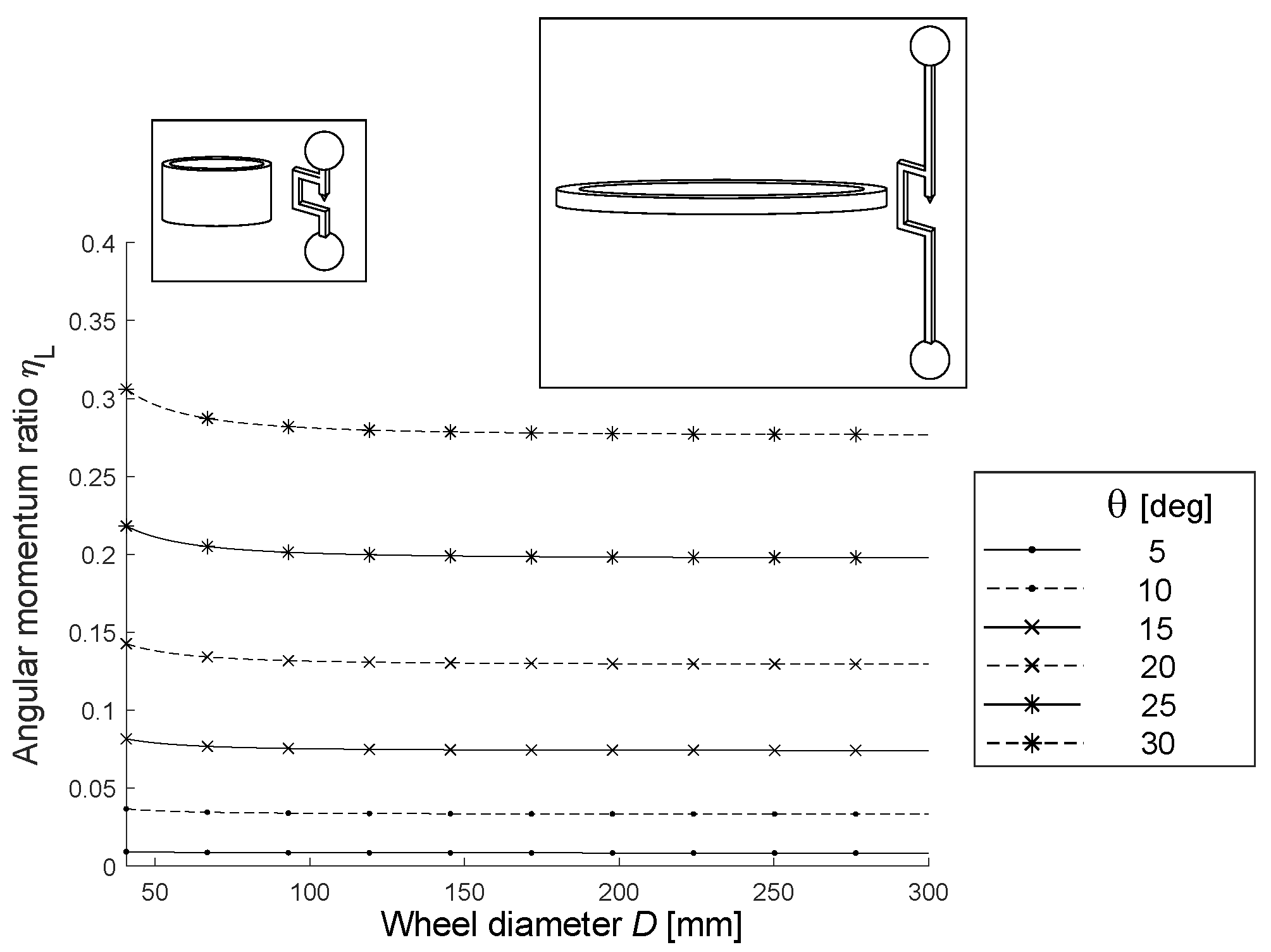
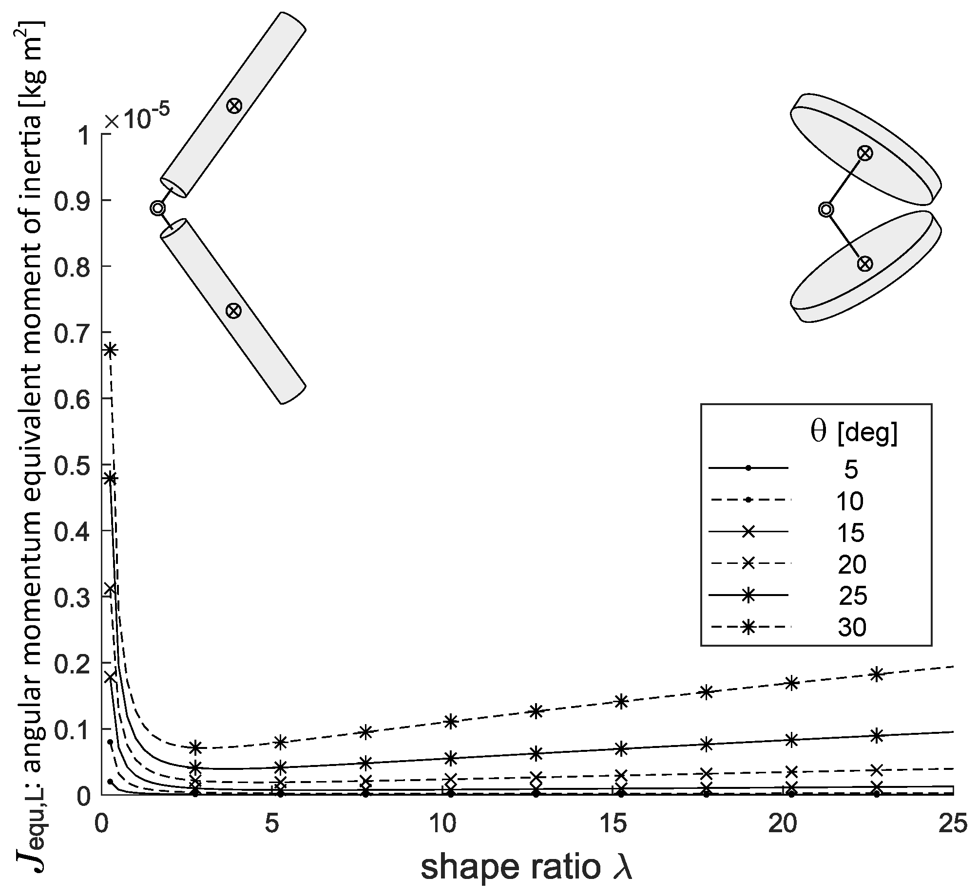
4. Influence of the Cylindrical Rigid Body Shape

Section 3 studies the influence of the flexure-based flywheel’s size and tilt amplitude on its angular momentum and kinetic energy, allowing a comparison to be drawn with a standard flywheel. This section explores instead the effect of the shape of the cylindrical rigid bodies. The dumbbell design, though more realistic, will be left aside, and pivoting cylinders (as shown in Figure 9) are considered instead (ss before, these cylinders are linked to the ground by CV joints located at their centers of mass). These cylinders have a radius R, a thickness t, and a fixed mass m (even though m has already been used to denote the sphere-shaped masses in Section 3, it will again be used here to avoid complex nomenclature). Their shape will be parameterized by their shape ratio $\lambda$:

$$\lambda =\frac{R}{t}.$$

(37)

The thickness t and radius R are given by

$$\begin{array}{c}\hfill t={\left(\frac{m}{\rho \pi {\lambda }^2}\right)}^{\frac{1}{3}}\mathrm{and}R={\left(\frac{\lambda m}{\rho \pi }\right)}^{\frac{1}{3}}.\end{array}$$

(38)

The resulting $J_{\mathrm{h}}$ and $J_{\mathrm{v}}$ are then as follows:

$$\begin{array}{cc}\hfill J_{\mathrm{h}}& =\frac{1}{12}m\left(3R^2+t^2\right)=\frac{m}{12}\left[{\left(\frac{m}{\rho \pi {\lambda }^2}\right)}^{\frac{2}{3}}+3{\left(\frac{\lambda m}{\rho \pi }\right)}^{\frac{2}{3}}\right],\hfill \end{array}$$

(39)

$$\begin{array}{cc}\hfill J_{\mathrm{v}}& =\frac{1}{2}m{R}^2=\frac{m}{2}{\left(\frac{\lambda m}{\rho \pi }\right)}^{\frac{2}{3}}.\hfill \end{array}$$

(40)

The resulting $J_{\mathrm{equ},\mathrm{L}}$ and $J_{\mathrm{equ},\mathrm{K}}$ are given by

$$\begin{array}{cc}\hfill J_{\mathrm{equ},\mathrm{L}}& =\frac{1}{6}\left(cos\theta -1\right)m{\left(\frac{m}{\rho \pi {\lambda }^2}\right)}^{\frac{2}{3}}\left(3cos\theta {\lambda }^2-3{\lambda }^2-cos\theta -1\right),\hfill \end{array}$$

(41)

$$\begin{array}{cc}\hfill J_{\mathrm{equ},\mathrm{K}}& =\frac{1}{6}\left(cos\theta -1\right)m{\left(\frac{m}{\rho \pi {\lambda }^2}\right)}^{\frac{2}{3}}\left(3cos\theta {\lambda }^2-9{\lambda }^2-cos\theta -1\right).\hfill \end{array}$$

(42)

The evolution of $J_{\mathrm{equ},\mathrm{L}}$ and $J_{\mathrm{equ},\mathrm{K}}$ with respect to $\lambda$ is shown in Figure 10 and Figure 11 for a selection of elevation angles $\theta$ and with $m=0.1$ kg out of steel ($\rho$ = 8000 kg m³):

Figure 10 shows that the most angular momentum is generated with small values of $\lambda$, which corresponds to elongated slender cylinders. Large values of $\lambda$, which correspond to thin flat disks, result in small angular momentum, with a minimum for intermediate values. Intuitively explained, long slender cylinders and flat disks have the mass distributed from the center of rotation, resulting in larger angular momentum. For cylindrical inertial bodies that are neither slender nor flat, their mass is close to the center, resulting in smaller angular momentum. Last, it can be seen that increasing the elevation angle $\theta$ increases the angular momentum.

Figure 11 shows that elongated slender cylinders store some kinetic energy, but flat disks store much more. There is also the same minimum for the same reason as for $J_{\mathrm{equ},\mathrm{L}}$, in which cylindrical rigid bodies are neither slender nor flat and have their mass distribution closer to their center of rotation. Similarly to $J_{\mathrm{equ},\mathrm{L}}$, increasing $\theta$ also increases the stored kinetic energy.

The most striking result of Figure 12 is that the equivalent moments of inertia $J_{\mathrm{equ},\mathrm{L}}$ and $J_{\mathrm{equ},\mathrm{K}}$ are different. Indeed, for a standard flywheel, the same graph as Figure 12 would be a flat line $y=1$. The fact that the ratio is not one means that the flexure-based flywheel can be seen as having two separate moments of inertia: one for the storage of angular momentum and the other for the storage of kinetic energy. Elongated cylinders have a ratio of approx. one, while thin flat disks have a ratio of approx. 100. This means that elongated cylinders have matching $J_{\mathrm{equ},\mathrm{L}}$ and $J_{\mathrm{equ},\mathrm{K}}$ and therefore behave identically to a standard flywheel. This joins the results of Equation (35) because elongated dumbbells fall in the same category as elongated slender cylinders. Thin flat disks, on the other hand, for the same amount of stored kinetic energy, generate approximately 100 times less angular momentum than a conventional flywheel would. This result leads to an interesting design consideration: if the goal of the flywheel is to generate angular momentum, then elongated cylinders are better suited, and if the goal is to store kinetic energy, then thin flat disks are optimal. This last property is interesting, as it leads to reduced gyroscopic forces if the flywheel’s axis is changed. Concerning the elevation angle $\theta$, the ratio is larger for smaller elevation angles. This does not mean, however, that smaller elevation angles store more kinetic energy but that they generate practically no angular momentum.

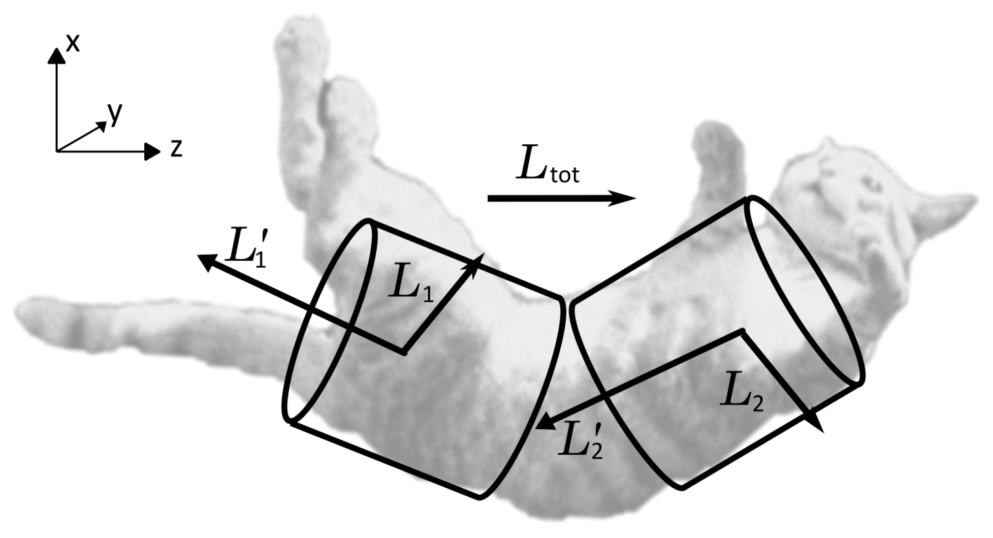
5. Analogy with a Falling Cat

It so happens that this flywheel design follows the mechanics of a falling cat, which re-orients itself during its fall in order to land on its feet. Among the different models of a falling cat proposed by the literature [8,9,10,11], Rademaker [9] considers a falling cat as two rolling cylinders that keep a constant relative bending angle (Figure 13). Each cylinder has its own oblique and constant angular momentum (${\mathit{L}}_1^{\prime }$ and ${\mathit{L}}_2^{\prime }$), resulting in a non-zero total angular momentum in the same manner as the proposed mechanism. Indeed, the two cylinders roll against each other without slipping, which implicitly assumes the presence of a CV joint linking them.

A difference between Rademaker’s model and the analysis presented in this work is the choice of the frame in which the angular momentum is evaluated. In Rademaker’s case, this frame keeps the bend between the two cylinders in the same orientation. If the same falling cat is similarly described in a frame fixed with respect to the cat’s waist, the two cylinders are no longer rolling around their respective axes but perform the same pivoting motion as the proposed mechanism.

The falling cat phenomenon has already found several applications in robotic attitude control. However, examples from the literature [13,14,15] require motorized joints to provide the pivoting motion, whereas this paper relies on passive mechanical means to guarantee the pivoting motion as well as the fixed elevation angle. Moreover, the presented mechanism truthfully follows the rolling cylinder model in contrast to other works in the literature [13,14], which use a Hooke joint instead of a CV joint.

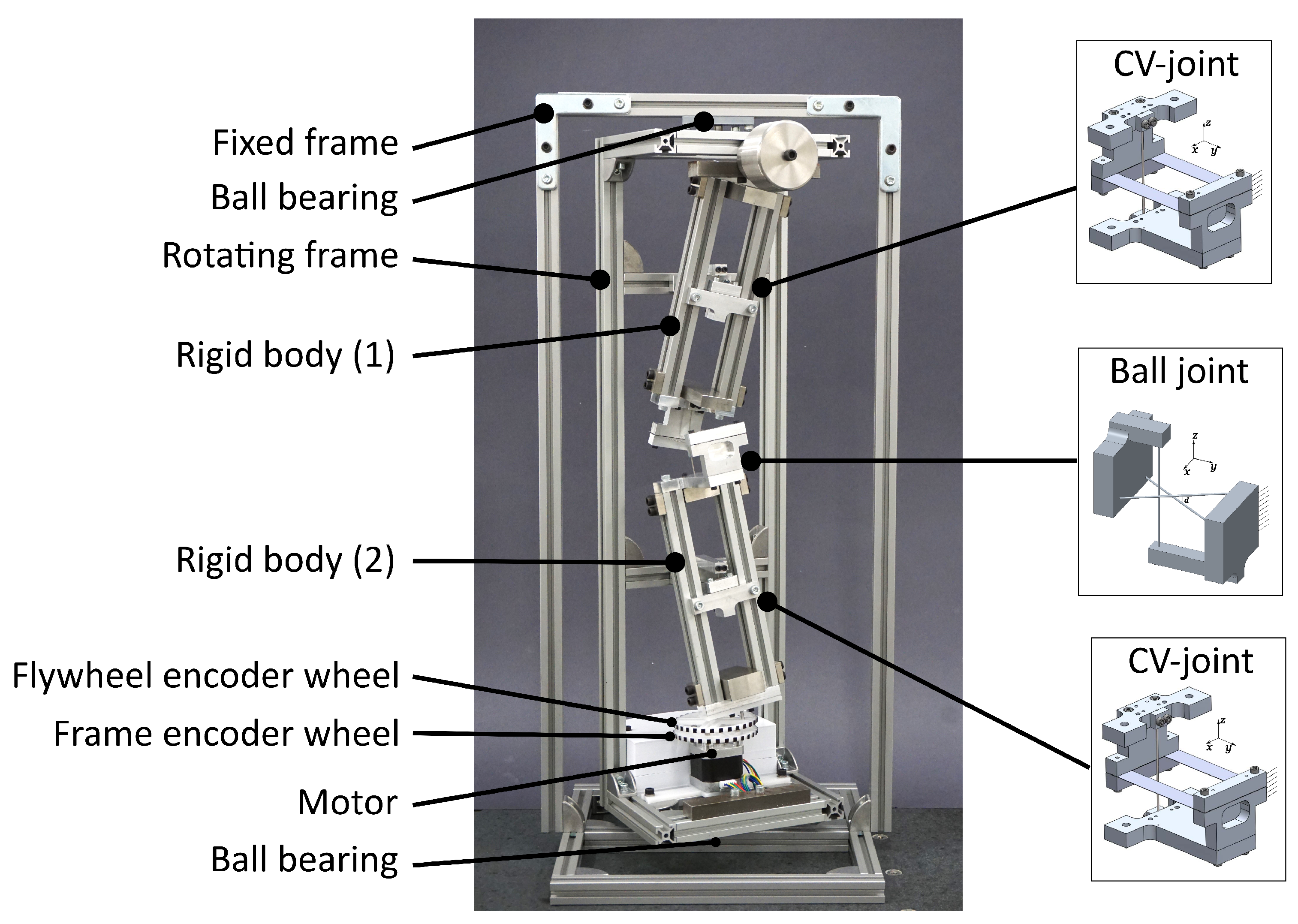
6. Demonstrator Prototype of the Flywheel

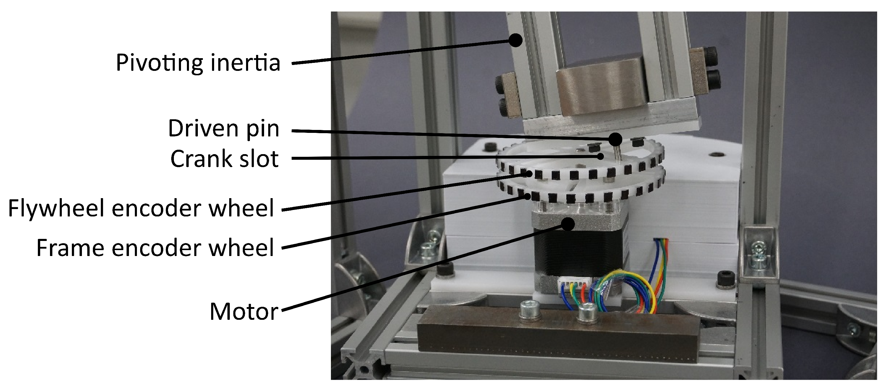
6.1. Constructed Demonstrator

A proof-of-concept demonstrator of the flywheel has been constructed with flexures and is shown in Figure 15. The flexures are designed so that their internal stress (flexion and traction when the mechanism is wobbling at three (RPS)) never overcomes their endurance limit. In this way, the fatigue effects will not impact the lifetime of the mechanism, which is theoretically infinite. The CV joints are constructed by means of a flexible rod parallel to the z-axis and a split flexible blade that lies in a plane parallel to the $xy$ planes (Figure 14a). The split blade, though technically overconstrained if considered as two independent blades, acts as a single blade and restricts translation in the x and y directions as well as rotation around the z-axis. The rod supports the mass in the z direction and blocks its translation along that axis. It should be noted that the exactitude with which this flexure joint follows the kinematics of a CV joint has not been investigated, as this joint is only used for a proof-of-concept demonstrator. The flexure ball joint consists of three askew flexible rods, as shown in Figure 14b. The first rod lies on the z-axis and restricts translation along this axis. The other two lie in two separate planes parallel to the $xy$ plane and restrict translation motion in the $xy$ plane (the separation between the planes by a distance d is to prevent collision between the two rods). The flywheel has a height of 400 mm, each rigid body has a weight of 1 kg, and the CV joints each have an amplitude of ±12.5^∘ (the ball joint therefore has an amplitude of ±25^∘).

6.2. Experimental Validation

To demonstrate that the physical demonstrator can generate angular momentum, we propose to measure it while it is used as a reaction wheel. A reaction wheel is a device used in spacecrafts to control their orientation. It consists of a motorized flywheel that, when accelerated in one direction, accelerates the rest of the spacecraft in the other direction via a reaction torque. The flywheel is used as a reaction wheel in the sense that its base is free to rotate, resulting in the conservation of angular momentum for the system consisting of the rotating base and flywheel. When an angular velocity variation $\mathrm{\Delta }\dot{\phi }$ is applied to the flywheel, this will result in a variation in the angular velocity of the base of the opposite sign due to conservation of angular momentum.

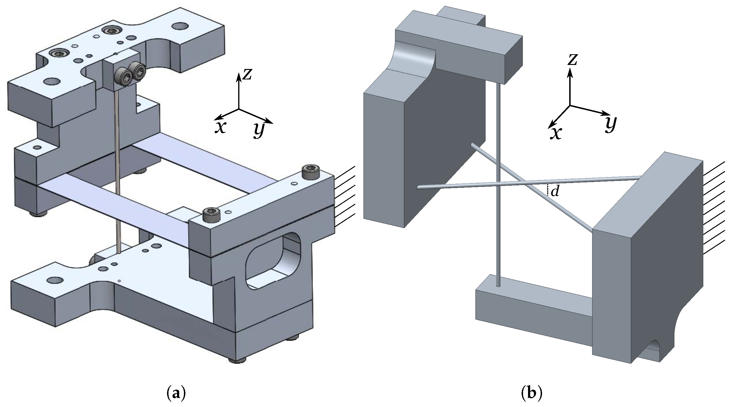
6.2.1. Experimental Setup

As the physical demonstrator only generates angular momentum along its z-axis, only the rotation of its base around this same axis is released. This was achieved with two ball bearings, as illustrated in Figure 15. In order to actuate the flywheel, a stepper motor has been added to the demonstrator. Its stator, along with its electronics, is fixed to the flywheel’s base, while its rotor drives a pin attached to the lower part of the rigid body (2) by means of a slotted crank (Figure 16). One can observe that the angular velocity of the motor’s rotor relative to its stator is equal to the parameter $\dot{\phi }$ used in the calculation of the angular momentum of the flywheel; see Section 2.3. In order to measure the rotational speeds of both the rotor and the rotating frame, encoding wheels have been attached to them and are observed by a high-speed camera, fixed in the inertial frame, at a 500 Hz frequency. A video of this experiment can be found at https://www.youtube.com/watch?v=tW9mJlxSyUs (accessed on 26 March 2024).

The motorized prototype as represented in Figure 15 has been set with the aforementioned elevation angle $\theta =12.5°$, and its principal moments of inertia are given in

Table 1. Principal moments of inertia of the demonstrator’s moving parts.

Description	Name	Value [kg· m2]
Horizontal inertia of the pivoting body	$J_{\mathrm{h}}$	$8.10·{10}^{-3}$
Vertical inertia of the pivoting body	$J_{\mathrm{v}}$	$8.54·{10}^{-4}$
Vertical inertia of the frame	$J_{\mathrm{f}}$	$3.03·{10}^{-2}$
Vertical inertia of the rotor	$J_{\mathrm{m}}$	$2.01·{10}^{-5}$

.

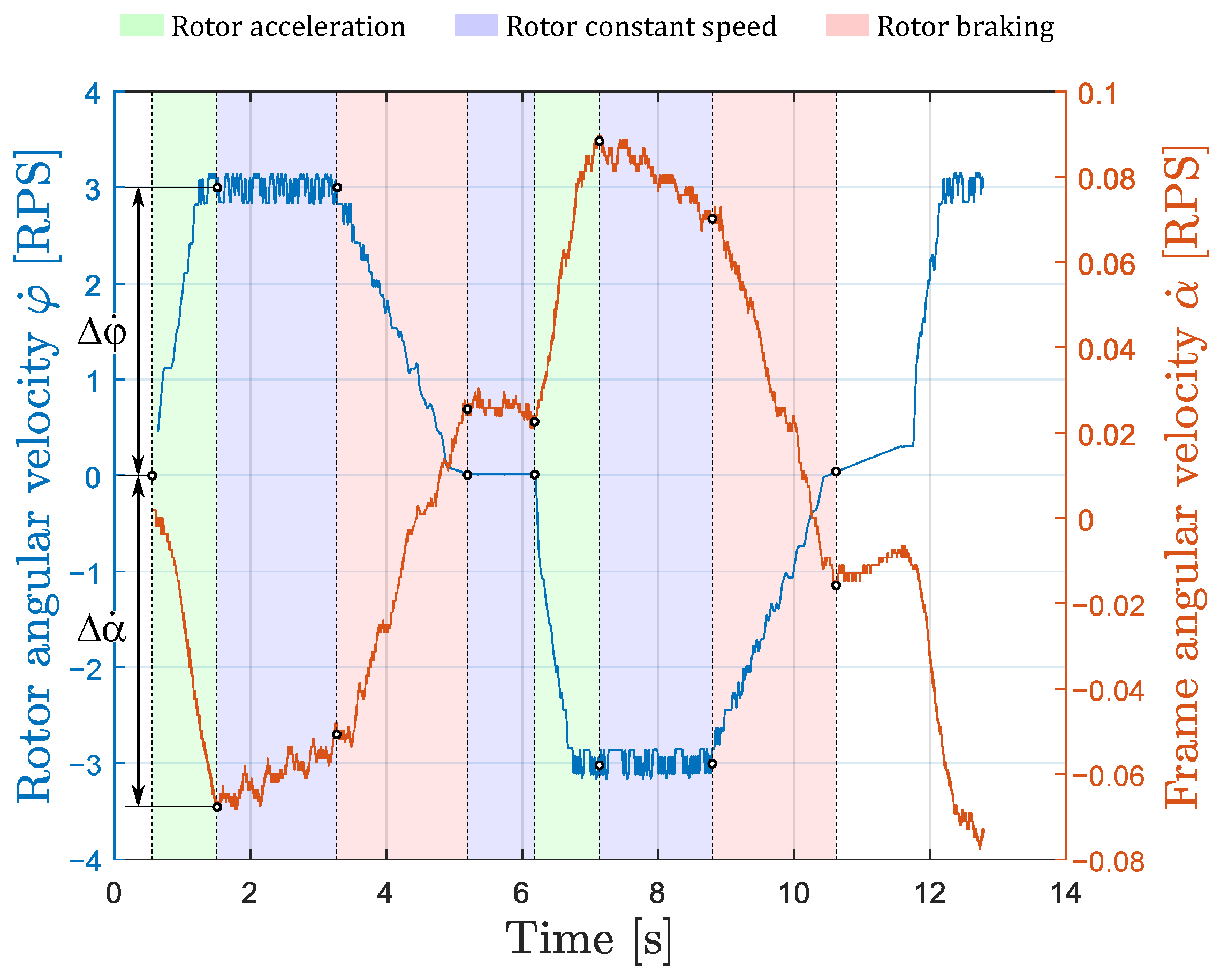
6.2.2. Experimental Results

The experimental measurements of the demonstrator are shown in Figure 17. The onboard rotor follows a repeating pattern: first, it accelerates to reach a positive speed of 3 [RPS], then it maintains that speed, and finally, it brakes to return to zero speed. This sequence is then reversed, and the two phases are repeated in an alternating manner. For each acceleration and braking phase, we first compute the change in angular velocities of the rotor and the frame, referred to as $\mathrm{\Delta }\dot{\phi }$ and $\mathrm{\Delta }\dot{\alpha }$, respectively. Then, the corresponding speed ratios $\mathrm{\Delta }\dot{\phi }/\mathrm{\Delta }\dot{\alpha }$ are calculated in order to be compared with the expected speed ratio from Equation (44). Note that we compute the speed ratios based on changes in speed rather than constant speed in order to be less dependent on friction, which tends to slow down the frame. The changes in angular velocities of the rotor and the frame and their corresponding speed ratios are gathered in

Table 2. Changes in angular velocities of the rotor and the frame with their corresponding velocity ratios for the acceleration and braking phases of the rotor.

	Acceleration 1	Braking 1	Acceleration 2	Braking 2
$\mathrm{\Delta }\dot{\phi }$ [RPS]	3.0	−3.0	−3.0	3.0
$\mathrm{\Delta }\dot{\alpha }$ [RPS]	−0.0683	0.0776	0.0656	−0.0849
$\frac{\mathrm{\Delta }\dot{\phi }}{\mathrm{\Delta }\dot{\alpha }}$ [/]	−43.9	−38.7	−45.7	−35.3

.

Considering the experimental setup presented in Figure 15, one can derive a formula that gives the speed ratio of the rotor’s angular velocity over the rotating frame’s angular velocity under the assessment of angular momentum conservation. The full development is given in the Appendix A, and the speed ratio that can be calculated is as follows:

$$\frac{\dot{\phi }}{\dot{\alpha }}=\frac{2\left(J_{\mathrm{v}}-J_{\mathrm{h}}\right){cos}^2\theta +J_{\mathrm{f}}+2J_{\mathrm{h}}+J_{\mathrm{m}}}{2\left(J_{\mathrm{h}}-J_{\mathrm{v}}\right){cos}^2\theta +2J_{\mathrm{v}}cos\theta -2J_{\mathrm{h}}-J_{\mathrm{m}}}.$$

(43)

By injecting into Equation (43) the elevation angle and the moments of inertia given in Table 1 from the previous section, this leads to the expected speed ratio:

$$\frac{\dot{\phi }}{\dot{\alpha }}=-44.15.$$

(44)

The results from Table 2 show good agreement between the expected and measured speed ratios with a relative difference of $7.4\%$. One can observe that, on average, the speed ratio’s amplitude for the acceleration phases is $21\%$ higher than the one from the braking phase. This difference can be explained by the presence of friction (bearings and air), which counteracts the frame’s acceleration during the acceleration phases and helps to decelerate the frame during the braking phases.

7. Discussion and Conclusions

This article introduces a flexure-based mechanism that successfully meets the essential criteria for a flywheel. Indeed, it is able to store kinetic energy and a constant angular momentum at a constant pivoting rate, it has a fixed center of mass and has zero force. A flexure-based implementation of the mechanism was shown, and the proof-of-concept prototype was successfully built and characterized in terms of reaction moment generation, which validates the analytical model. Note that this mechanism is not limited to reaction wheel applications. If coupled with a suitable variable transmission unit and clutch, whose designs are out of the scope of this manuscript, it can theoretically be used as a KERS flywheel for KERS applications.

In comparison to standard flywheels that use other types of bearings (such as ball bearings, magnetic bearings, and air bearings), the advantages of this flexure design are the absence of wear and lubrication, its low power consumption, its vacuum compatibility, and the possibility of miniaturization. The price to pay for these advantages is a six-fold reduction in kinetic energy and angular momentum storage capacity for a given mass, as well as a ten-fold increase in volume.

A particularity of this flexure-based flywheel is that the shape of the pivoting rigid bodies influences the ratio of kinetic energy versus angular momentum stored in the mechanism. Rigid bodies with an elongated cylindrical shape have the same ratio as classical flywheels, whereas those that have the shape of a flat disk store up to 100 times more kinetic energy for the same angular momentum as classical flywheels. This could be advantageous for kinetic energy storage applications where angular momentum is undesired, for example, due to the induced gyroscopic forces.

Hence, although comparatively heavy and cumbersome, the novel flexure-based flywheel offers interesting design features that might be key to specific applications in extreme environments.

References

1. Mathews, T.; Nishanth, D. Flywheel Based Kinetic Energy Recovery Systems (KERS) Integrated in Vehicules. IJEST 2013, 5, 1694–1699, ISSN: 0975-5462. [Google Scholar]
2. Heindel, S.; Liebold, F.; Sander, L. A Gas Bearing Reaction Wheel Supplied by Ultrasonic Pumps. In Proceedings of the 19th European Space Mechanisms and Tribology Symposium 2021, Online, 20–24 September 2021. [Google Scholar]
3. Gerlach, B.; Ehinger, M.; Seiler, R. Low noise five-axis magnetic bearing reaction wheel. In Proceedings of the International Federation of Automatic Control (IFAC), Heidelberg, Germany, 15 September 2006. [Google Scholar] [CrossRef]
4. Cosandier, F.; Henein, S.; Richard, M.; Rubbert, L. The Art of Flexure Mechanism Design; EPFL Press: Lausanne, Switzerland, 2017; ISBN 978-2-940222-56-8. [Google Scholar]
5. Flückiger, P.; Henein, S.; Vardi, I.; Schneegans, H.; Tissot-Daguette, L. Flexure wheels for spacecraft attitude control. Eng. Arch. 2021. pre-print. [Google Scholar] [CrossRef]
6. Schneegans, H.; De Jong, J.; Cosandier, F.; Henein, S. Mechanism Balancing Taxonomy. Mech. Mach. Theory 2024, 191, 105518. [Google Scholar] [CrossRef]
7. Vardi, I.; Rubbert, L.; Bitterli, R.; Ferrier, N.; Kahrobaiyan, M.; Nussbaumer, B.; Henein, S. Theory and design of spherical oscillator mechanisms. Precis. Eng. 2018, 51, 499–513. [Google Scholar] [CrossRef]
8. Guyou, M. Note relative à la communication de M. Marey. C. R. Acad. Sci. 1894, 119, 717–718. [Google Scholar]
9. Rademaker, G.G.J.; Ter Braak, J.W.G. Das Umdrehen der fallenden Katze in der Luft. Acta Oto-Laryngol. 1936, 23, 313–343. [Google Scholar] [CrossRef]
10. Kane, T.R.; Scher, M.P. A dynamical explanation of the falling cat phenomenon. Int. J. Solids Struct. 1969, 5, 663–670. [Google Scholar] [CrossRef]
11. Cao, J.; Wang, S.; Zhu, X.; Song, L. A Review of Research on Falling Cat Phenomenon and Development of Bio-Falling Cat Robot. In Proceedings of the 4th WRC Symposium on Advanced Robotics and Automation 2022, Beijing, China, 20 August 2022. [Google Scholar] [CrossRef]
12. Crane, R. A Cat Being Dropped Upside Down. Available online: https://www.shutterstock.com/editorial/image-editorial/cat-being-dropped-upside-down-demonstrate-how-12360717d (accessed on 18 March 2024).
13. Mather, T.W.; Yim, M. Modular configuration design for a controlled fall. In Proceedings of the 2009 IEEE/RSJ International Conference on Intelligent Robots and Systems, St. Louis, MO, USA, 11–15 October 2009. [Google Scholar] [CrossRef]
14. Crews, S.; Agrawal, S.; Velado, S. CatAstroΦ—Inertial Reorientation of a Freely Falling Cat Using Nonholonomic Motion Planning. Available online: https://www.youtube.com/watch?v=rq2wpRNUbDI (accessed on 18 March 2024).
15. Garant, X.; Gosselin, G. Design and Experimental Validation of Reorientation Manoeuvres for a Free Falling Robot Inspired from the Cat Righting Reflex. IEEE Trans. Robot. 2021, 37, 482–493. [Google Scholar] [CrossRef]
Figure 1. The inertial bodies considered in this paper: spherical inertial body (left), cylindrical inertial body (center), and dumbbell (right). This dumbbell has its mass concentrated exclusively in the two sphere-shaped masses (the mass of the rigid arms linking them are neglected), and the dumbbell effectively acts as a cylindrical inertial body. The center of mass (COM) of each body is highlighted, and it is assumed that the principal axes of inertia coincide, respectively, with the x-, y-, and z-axes. It can be seen that the cylinder and dumbbell have the same inertia tensor.
Machines 12 00232 g001
Figure 2. Sequential rotations with Euler angles φ , θ , and ψ , designated respectively as azimuth, elevation, and twist. The rotation sequence is first rotation φ around axis i , then rotation θ around n , and finally rotation ψ around v .
Machines 12 00232 g002
Figure 3. Sequence of the flywheel design. It can be seen that at each step, the bodies’ angular momenta L 1 and L 2 are oblique and result in a total angular momentum L tot . Note that ω 1 and L 1 and, respectively, ω 2 and L 2 , lie in the same vertical plane but are only colinear in the case of spherical inertia.
Machines 12 00232 g003
Figure 4. Rigid body 1 is isolated from the rest of the mechanism. The internal forces T and T are respectively applied to its ball joint and CV joint. The net torque M 1 , equal to L ˙ 1 , the time derivative of L 1 , is also highlighted.
Machines 12 00232 g004
Figure 5. Standard flywheel and flexure-based flywheel used for the performance comparison. The standard flywheel’s diameter D matches the dumbbell’s length (i.e., the distance between the centers of the sphere-shaped masses). The cylindrical envelope of the flexure-based flywheel is also highlighted and encompasses the whole mechanism, including the dumbbells’ spheres.
Machines 12 00232 g005
Figure 6. Angular momentum ratio η L as a function of flywheel diameter D. The flywheel and dumbbell illustrations show the overall appearance for the different diameters D (not to scale).
Machines 12 00232 g006
Figure 7. Kinetic energy ratio η K as a function of flywheel diameter D. The flywheel and dumbbell illustrations show the overall appearance for the different diameters D (not to scale).
Machines 12 00232 g007
Figure 8. Volume ratio η V as a function of flywheel diameter D. The flywheel and dumbbell illustrations show the overall appearance for the different diameters D (not to scale).
Machines 12 00232 g008
Figure 9. The studied pivoting cylindrical inertial bodies. As before, the cylindrical rigid bodies are fixed to the base via CV joints and linked together via a ball joint.
Machines 12 00232 g009
Figure 10. J equ , L as a function of shape factor λ . The two illustrations of the cylindrical inertial bodies show the overall appearance of the system for the different values of λ (not to scale).
Machines 12 00232 g010
Figure 11. J equ , K as a function of shape factor λ . The two illustrations of the cylindrical rigid bodies show the overall appearance of the system for the different values of λ (not to scale).
Machines 12 00232 g011
Figure 12. J equ , K / J equ , L as a function of shape factor λ . The two illustrations of the cylindrical rigid bodies show the overall appearance of the system for the different values of λ (not to scale).
Machines 12 00232 g012
Figure 13. A falling cat seen as two rolling cylinders. In a frame where the cylinders rotate around their axes, they have angular momenta L 1 and L 2 . When in a frame fixed with respect to the cat’s waist, the cylinders pivot and have angular momenta L 1 and L 2 , which lead to an overall angular momentum L tot . (Image adapted from [12].)
Machines 12 00232 g013
Figure 14. CAD views of the prototype’s implemented flexure-based (a) CV joint, which enables the upper part to pivot around the x- and y-axes and (b) ball joint, which connects the two inertial pivoting bodies. Note: the two rods parallel to the x y -plane lie in two distinct planes separated by a distance d.
Machines 12 00232 g014
Figure 15. Constructed demonstrator with the different components and joints highlighted.
Machines 12 00232 g015
Figure 16. Measurement setup with the different components highlighted.
Machines 12 00232 g016
Figure 17. Angular velocities of the rotor ( φ ˙ ) and the frame ( α ˙ ) with respect to the time. The rotor acceleration, constant speed, and braking phases are identified using green, blue, and red colors, respectively. The changes in angular velocity φ ˙ and α ˙ are highlighted for the first acceleration phase.
Machines 12 00232 g017