Article

Research on the Control Method of a Brushless DC Motor Based on Second-Order Active Disturbance Rejection Control

Beijing Engineering Research Center of Precision Measurement Technology and Instruments, Beijing University of Technology, No. 100, Pingleyuan, Chaoyang District, Beijing 100124, China
*
Author to whom correspondence should be addressed.
Machines 2024, 12(4), 244; https://doi.org/10.3390/machines12040244
Submission received: 25 February 2024 / Revised: 3 April 2024 / Accepted: 6 April 2024 / Published: 8 April 2024
(This article belongs to the Special Issue Design and Control of Electrical Drives and Electrical Machines)

Abstract

:
This research addresses the issues of weak anti-disturbance ability, fast response, and incompatibility of overshoot in the control process of brushless DC motors (BLDCs). A six-step commutation control method based on second-order active disturbance rejection control (ADRC) is derived following the analysis of the BLDC model and the mathematical model of ADRC. A control model of the BLDC using both PI and ADRC is constructed. Detailed comparative and quantitative analyses of the simulation results using PI and ADRC are conducted, focusing on the anti-load disturbance capabilities using the integrated square error (ISE), integrated time square error (ITSE), integrated absolute error (IAE), and integrated time absolute error (ITAE). Experimental testing on the STM32F4 controller is also carried out, analyzing four error integral criteria in depth. The results indicate that both the ADRC and PI control modes can track the target signal without overshooting, demonstrating strong anti-load disturbance ability and robustness at varying working speeds. In the BLDC control system, using the ADRC control method can achieve fast and non-overshoot tracking of target signals compared to the PI control method, and ADRC has stronger resistance to load disturbances.

1. Introduction

The brushless DC motor (BLDC), utilizing Hall sensors as opposed to the mechanical commutators found in traditional DC motors, offers high efficiency, low noise, superior torque characteristics, and a simple structure, with a wide speed regulation range. Its applications include new energy automobiles, numerical control systems, flight control systems, ships, home appliances, and medical equipment [1,2,3,4,5].
The control process of DC brushless motors can be classified into inductive control and non-inductive control based on the presence or absence of position sensors. Vector control strategies are typically used for brushless DC motors without position sensors. The FOC control method or six-step commutation method can be used in the process of position sensor control. For brushless motors with only an encoder installed, the FOC control method is generally used. For brushless motors with only three-phase Hall sensors installed, a six-step commutation method is generally used for control. This article mainly focuses on brushless motors equipped with Hall sensors for sampling and six-step commutation control. This paper explores the two-by-two conduction mode six-step phase change method control of BLDC. Advances in structural design and permanent magnet materials, in addition to improved control strategies, can significantly enhance control performance. Despite the simplicity and ease of implementation of the proportion integration differentiation (PID) control mode, it struggles with the nonlinear nature and variable load disturbances of BLDC, prompting research into alternative methods such as fuzzy PID, neural network PID, enhanced PID control, and sliding-mode variable structure control [6,7,8,9,10,11].
The study detailed in [12] integrates a fuzzy control algorithm with a PID controller, assessing its efficacy in mitigating speed and torque fluctuations in brushless DC (BLDC) motors through simulation for improved performance. Reference [13] described the use of the particle swarm optimization algorithm to fine-tune PID control parameters, resulting in enhanced response characteristics, minimized steady-state error, and reduced overshoot. Control of BLDC motors can be achieved using artificial intelligence approaches without requiring detailed parameters. According to [14], the application of neural networks, genetic algorithms, and artificial intelligence methods in brushless DC motor technology provides valuable guidance and references for researchers in the BLDC drive domain. Moreover, [15] demonstrated the combination of fuzzy logic and fuzzy logic to improve response speed and disturbance resistance. The approach in [16] presented the use of a fuzzy control strategy to adjust the parameters of a sliding mode controller based on an FPGA controller, thereby improving the control performance of BLDC motors.
BLDC systems are complex, multivariable control systems prone to issues such as load perturbation and parameter variations during operation. Han Jingqing, a scholar at the Chinese Academy of Sciences, developed a novel control technology known as self-imposed perturbation control, grounded in a comprehensive analysis of both modern and classical control theories. ADRC has strong robustness, good adaptability, and excellent tracking characteristics. The ESO in ADRC estimates all influencing factors in the system and achieves real-time dynamic adjustment through NLSEF, thus effectively resisting various interferences and uncertain factors. The ADRC does not rely on the precise mathematical model of the controlled object, meaning it performs well in dealing with model uncertainty and external disturbances. TD in ADRC can achieve fast and non-overshoot tracking of target signals, enabling ADRC to achieve more accurate and rapid tracking. This method, using the integral series type as a benchmark, addresses the total perturbations of the system, including uncertainty and internal and external perturbations. These perturbations are estimated and eliminated in real-time by expanding the state observer, simplifying the nonlinear object full of perturbations and uncertainty to a standard series type. This control technique exhibits exceptional performance in both dynamic and static settings, with strong perturbation resistance. Since its inception, active disturbance rejection control (ADRC) technology has attracted considerable attention and has been rapidly implemented in various control sectors, including industrial control [17], robotics [18,19], new energy vehicles [20,21], aircraft [22,23], and aerospace [24,25].
The approach in [26] discussed the use of an enhanced self-immunity controller to reduce torque pulsation in BLDC. The approach in [27] details the implementation of ADRC in a flywheel storage system to improve its immunity and dynamic characteristics. The approach in [28] reports the application of a third-order ADRC for speed control of an asynchronous motor, with its effectiveness validated in a DSP controller. These experimental outcomes highlight the method’s ability to enhance the robustness of asynchronous motor speed. BLDC motors are employed as driving components in optical scanning systems. According to the approach in [29], ADRC was implemented to facilitate the transition between “point-to-point control” and “stable speed control”. In [30], a combination of a neural network and ADRC controllers was utilized, with the ADRC parameters adjusted in real-time to improve the control precision of the BLDC servo system. Reference [31] applied ADRC to the BLDC two-wheeled balance car system to augment balance stability and robustness. However, the literature [30,31] did not establish a simulation model for the BLDC six-step commutation method, nor did it quantitatively analyze the load disturbance resistance characteristics of the PI control method and ADRC control method.
This paper presents a BLDC speed control strategy employing second-order ADRC, following an analysis of the mathematical models of BLDC and ADRC. This research involves establishing a simulation model for BLDC based on ADRC, followed by a comprehensive comparison and analysis of the simulation results of control based on ADRC and PID. The disturbance resistance of the system is quantitatively assessed using the integrated time absolute error (ITAE) and integrated absolute error (IAE) guidelines. Experimental tests on the STM32F4 controller demonstrate that the control method offers rapid response speed and high resistance to load disturbances. In the BLDC control system, the ADRC can achieve fast and non-overshoot tracking of target signals compared to the PI control method and has stronger resistance to load disturbances.

2. Mathematical Model of BLDC

In BLDC motors, each opposing electromotive force exhibits a trapezoidal wave, and the mutual inductance between the stator and rotor is non-sinusoidal. Therefore, direct use of the d-q coordinate transformation for BLDC three-phase equations is not feasible. The mathematical model of the BLDC is established based on the relationships among its inherent variables. The interaction between permanent magnets and windings, as well as between the windings themselves during operation, combined with magnetic circuit saturation and other nonlinear factors, results in a complex electromagnetic relationship.
BLDC motors are nonlinear, highly coupled multivariable systems. Using a three-phase global inverter circuit with a two-two conduction mode, the following assumptions are made without compromising the control effect: symmetric distribution of the stator current and magnetic field; exclusion of eddy current and hysteresis losses; and neglect of cogging and the armature reaction. The equation for the stator voltage can be expressed as follows:
u a u b u c = R s 0 0 0 R s 0 0 0 R s i a i b i c + d d t L a L a b L a c L b a L b L b c L c a L c b L c i a i b i c + e a e b e c
The voltages of the three phases are given as ua, ub, and uc, while ea, eb, and ec represent the respective reverse electromotive forces. The currents of the phases can be given as ia, ib, and ic. La, Lb, and Lc refer to the inductances of the three-phase windings. Lab indicates the mutual inductance of the AB phase winding. The rotor comprises a permanent magnet, and the influence of the rotor can be discounted. Thus, La = Lb = Lc = L, and Lab = Lba = Lac = Lca = Lbc = Lcb = M, where M represents the mutual inductance of the windings. The stator’s three-phase windings are connected in a Y-formation, leading to the following relationship.
i a + i b + i c = 0 M i a + M i b + M i c = 0
Equation (1) can be simplified as
u a u b u c = R s 0 0 0 R s 0 0 0 R s i a i b i c + d d t L M 0 0 0 L M 0 0 0 L M i a i b i c + e a e b e c
According to Equation (3), the equivalent circuit of the BLDC motor is shown in Figure 1.
Torque equation.
T e = [ e a i a + e b i b + e c i c ] / ω
The electromagnetic torque, Te, can be controlled by adjusting the amplitude of the square wave current in the BLDC motor. During operation, the stator only conducts in a two-by-two pattern. The expression for electromagnetic power is outlined as follows:
P e = e a i a + e b i b + e c i c = 2 E s I s
The steady-state value of the opposing electromotive force when the two terminals are active is denoted as Es, and the phase current of the winding at steady state is referred to as Is.
If mechanical losses and other stray losses of the motor are disregarded, all the electromagnetic power is converted into rotor kinetic energy.
P e = T e ω
Then, Equation (4) can be transformed into
T e = 2 E s I s ω = K t I s       T e = 2 E s I s ω = K t I s
where Kt represents the coefficient of motor torque.
The equation of motion for a BLDC motor is as follows:
J d ω d t = T e T L B ω
where TL is the load torque, J is the rotational inertia, and B is the damping factor.

3. Second-Order ADRC Construction of the BLDC Speed Loop

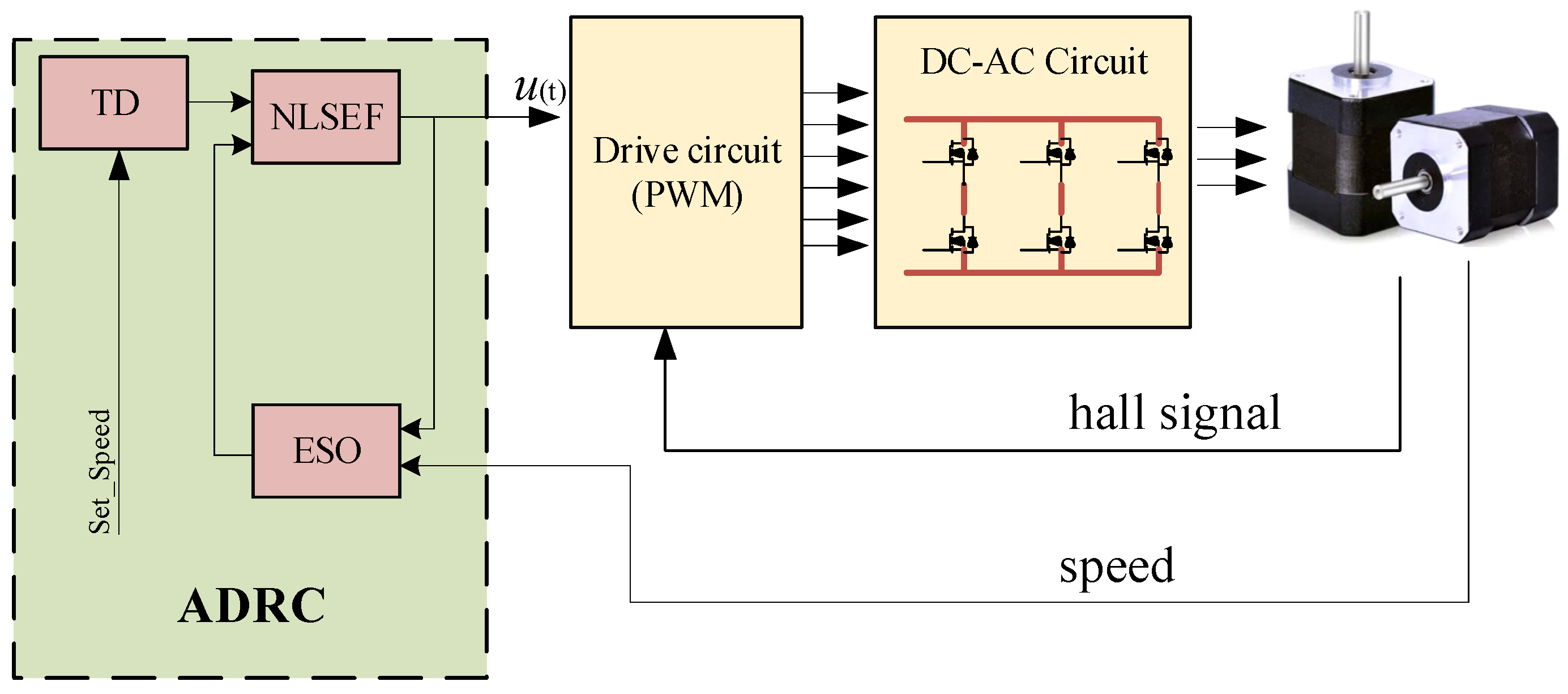
3.1. Second-Order ADRC Control Principle

The PID control structure is frequently utilized for the BLDC speed loop control procedure. Equation (9) presents the structure
u ( t ) = k p e ( t ) + k i 0 t e ( t ) d t + k d d e ( t ) d t
In the PID controller, the proportional link effectively regulates the BLDC’s response speed. However, increasing kp can lead to overshooting. It is crucial to find an optimal balance between kp and Ki to achieve optimal performance. The integral link can eliminate steady-state error in the system, and increasing ki can accelerate the error reduction. However, an excessively large ki can cause integral saturation. When connected to a system error, the differential link suppresses overshooting. Increasing kd prolongs the system regulation time, thereby weakening the disturbance resistance of the system. However, the PID controller struggles to harmonize with fast or overshooting dynamics, resulting in diminished disturbance resistance.
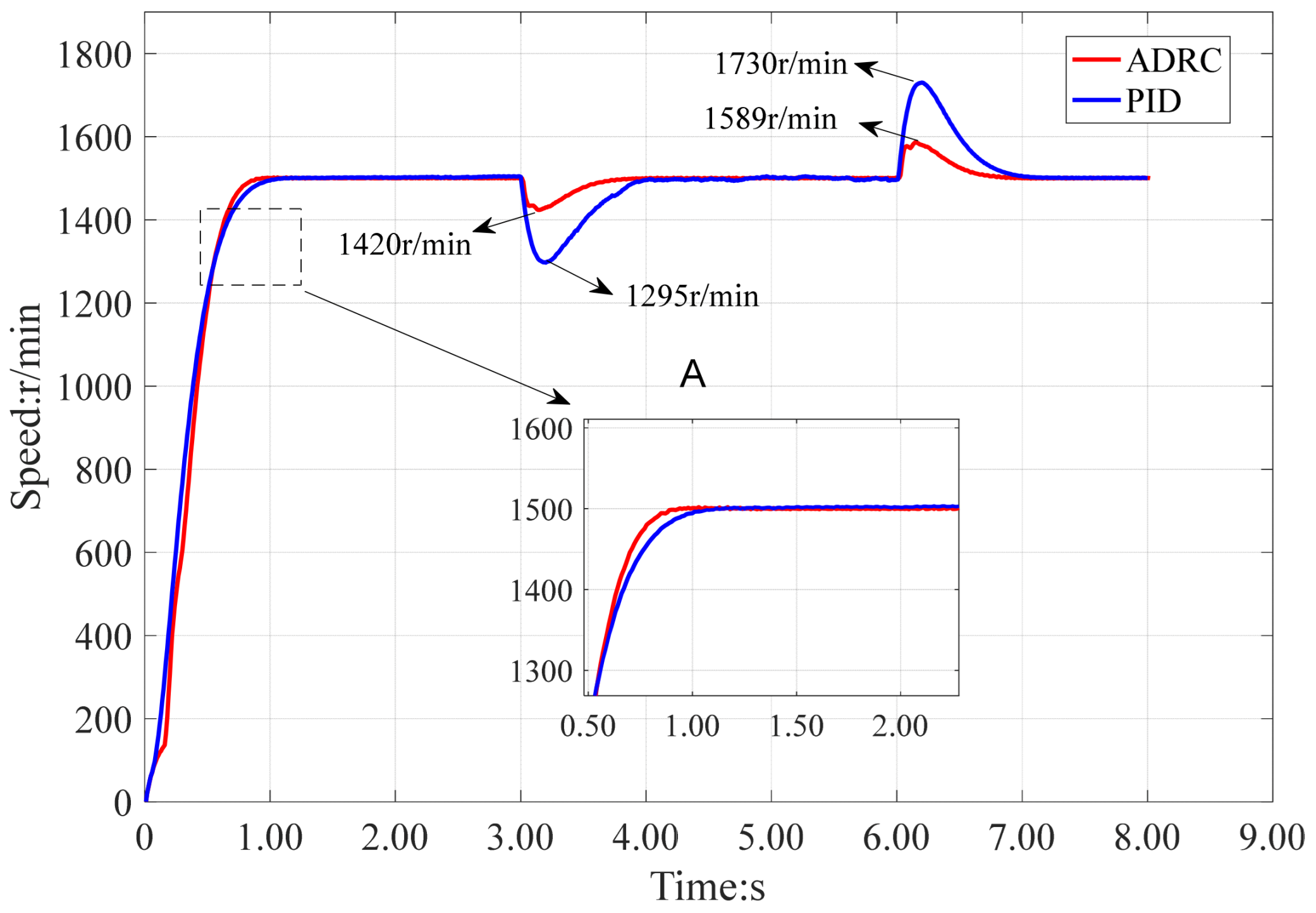
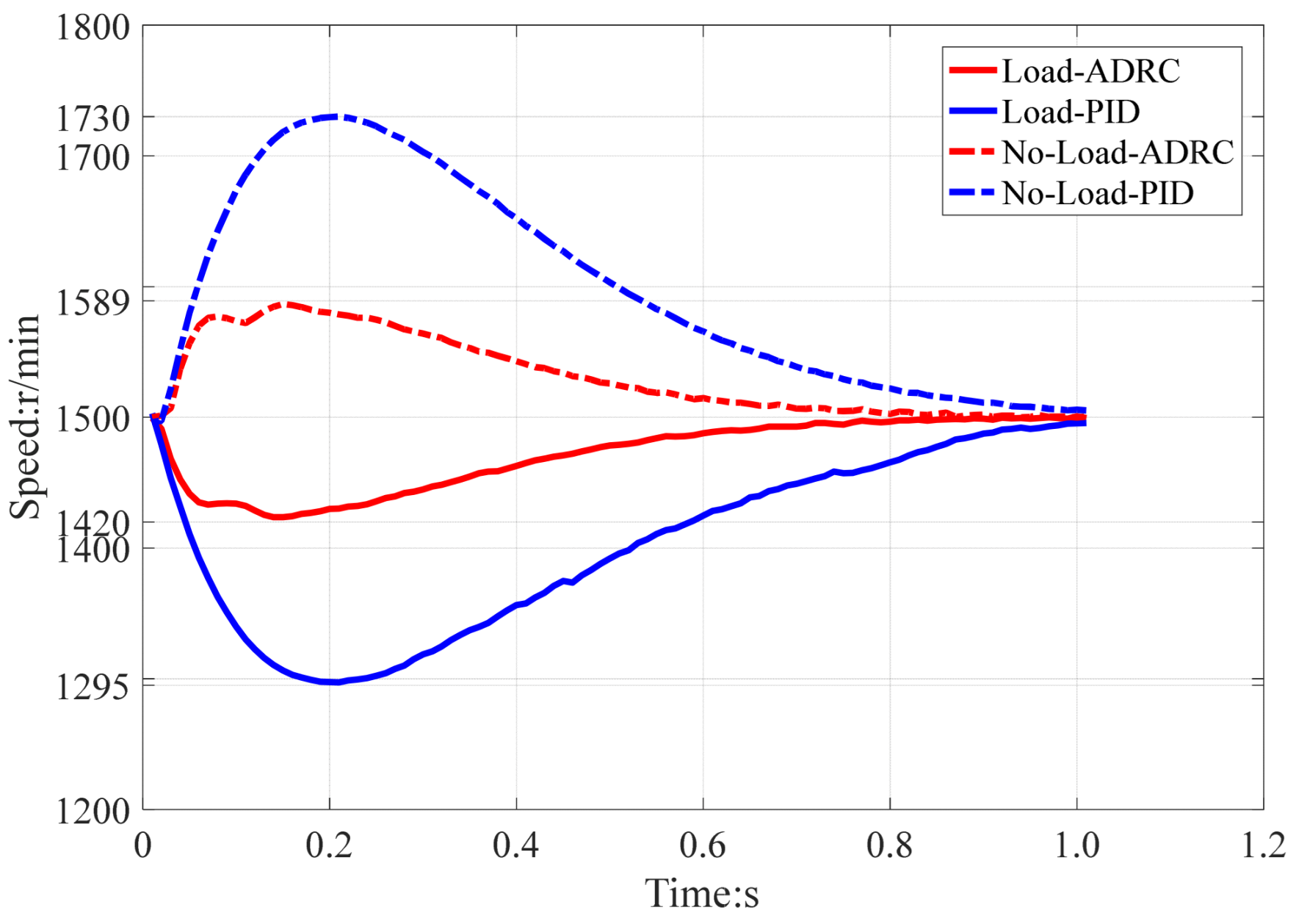
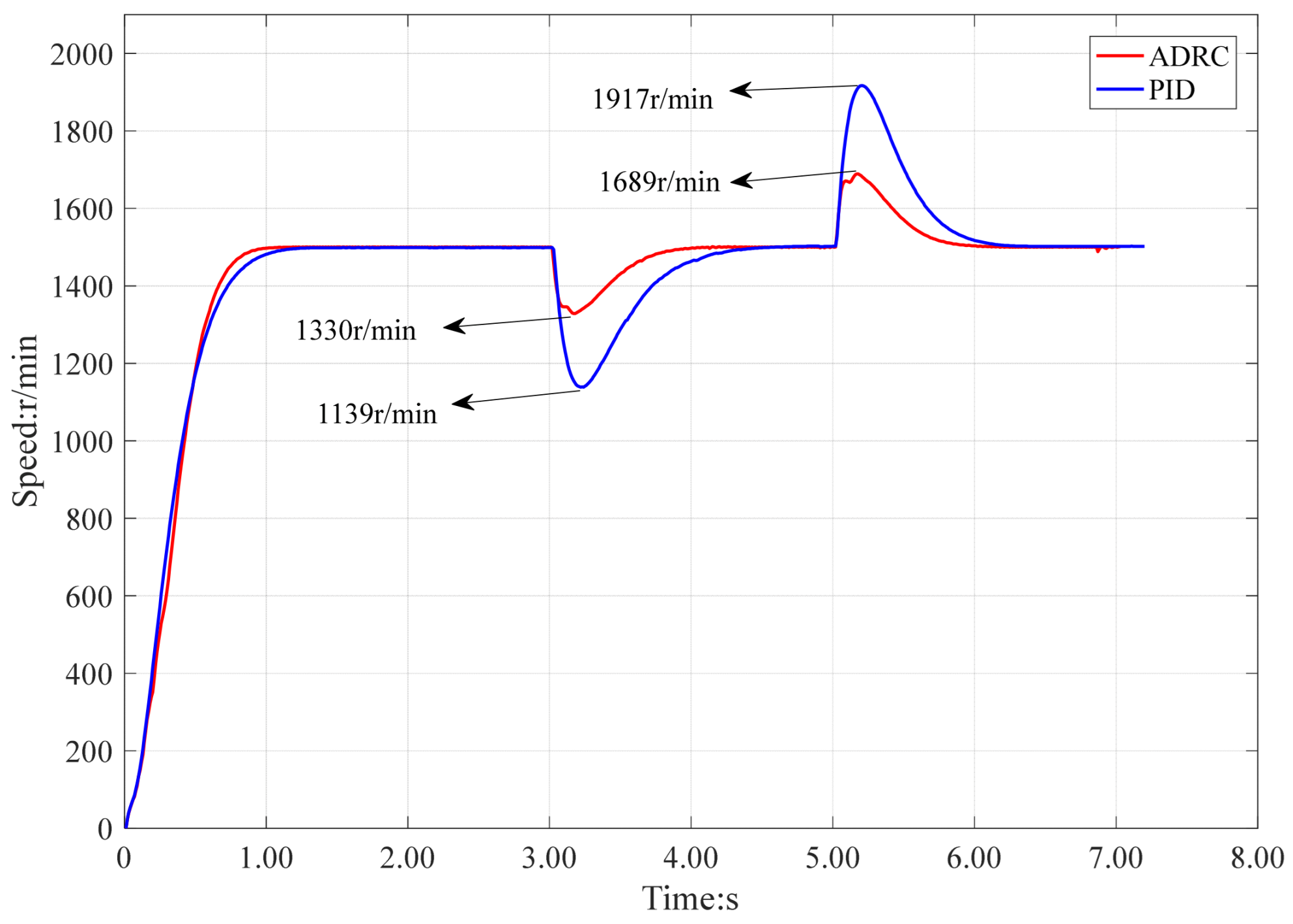
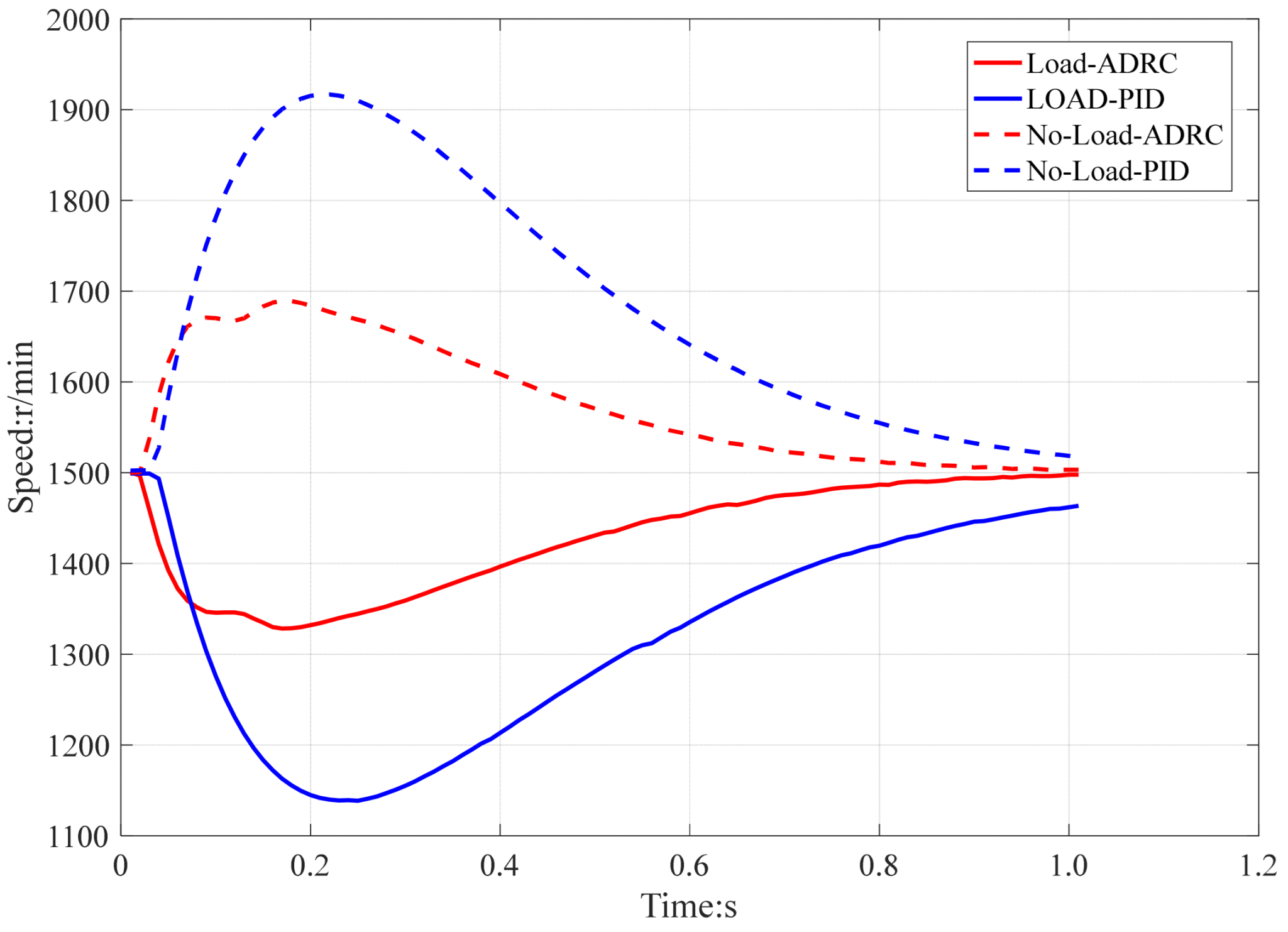
The ADRC is a high-performance nonlinear control technique that evolved from PID and modern control theory. The ADRC does not require precise mathematical models of controlled objects. Instead, it assesses and corrects total disturbances by evaluating the combined effect of the “uncertain model part” and “unknown disturbances” as the total disturbance. The ADRC controller comprises a tracking differential (TD), an extended state observer (ESO), and nonlinear state error feedback (NLSEF), in addition to a new controller. NLSELF can observe and compensate for the system’s uncertain model parts and unknown perturbations. Compared to the PID controller, the ADRC is more adept at meeting the control requirements of nonlinear complex systems, achieving rapid and overshoot-free responses in accordance with the target signal and exhibiting robust load disturbance resistance.
The primary function of the tracking differentiator is to manage the transition process, enabling fast and overshoot-free tracking of the target signal. TD effectively addresses the challenge of extracting continuous and differential signals from a discontinuous rotational speed signal replete with random noise.
The expanded state observer, a core component of ADRC, addresses the central issue of perturbation observation in active disturbance techniques. The ESO expands the perturbation action in the system into a new state variable and establishes a state observer capable of monitoring this expanded state. By utilizing a feedback mechanism, the ESO observes system perturbations and compensates for them at the control rate, thereby enhancing the system’s anti-disturbance capability. Importantly, expanded state observers do not rely on a specific model and do not require direct measurements to observe perturbations and obtain estimates.
The nonlinear state error feedback permits the combination of three signals—the error signal of the transition process, the integral signal of the error, and the differential of the error signal—either linearly or nonlinearly. By utilizing the nonlinear fal(·) function, NLSEF achieves the control effect of “small error, large gain; large error, small gain”, thereby enhancing the robustness and adaptability of the system.
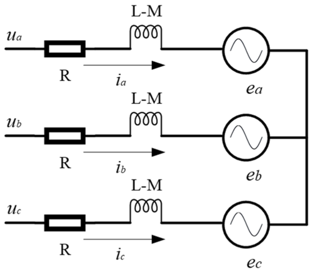
The differential equation for an uncertain object subject to an unknown perturbation is expressed as follows:
x ˙ 1 ( t ) = x 2 ( t )                     x ˙ n 1 ( t ) = x n ( t ) x n = f ( x , x ˙ , ~ , x ( n 1 ) , t ) + d ( t ) + b u ( t ) y = x 1 ( t )
where f(x, x1, ~, x(n−1), t) is the unknown function, d(t) is the unknown perturbation, y is the system output, and u(t) is the system control quantity.
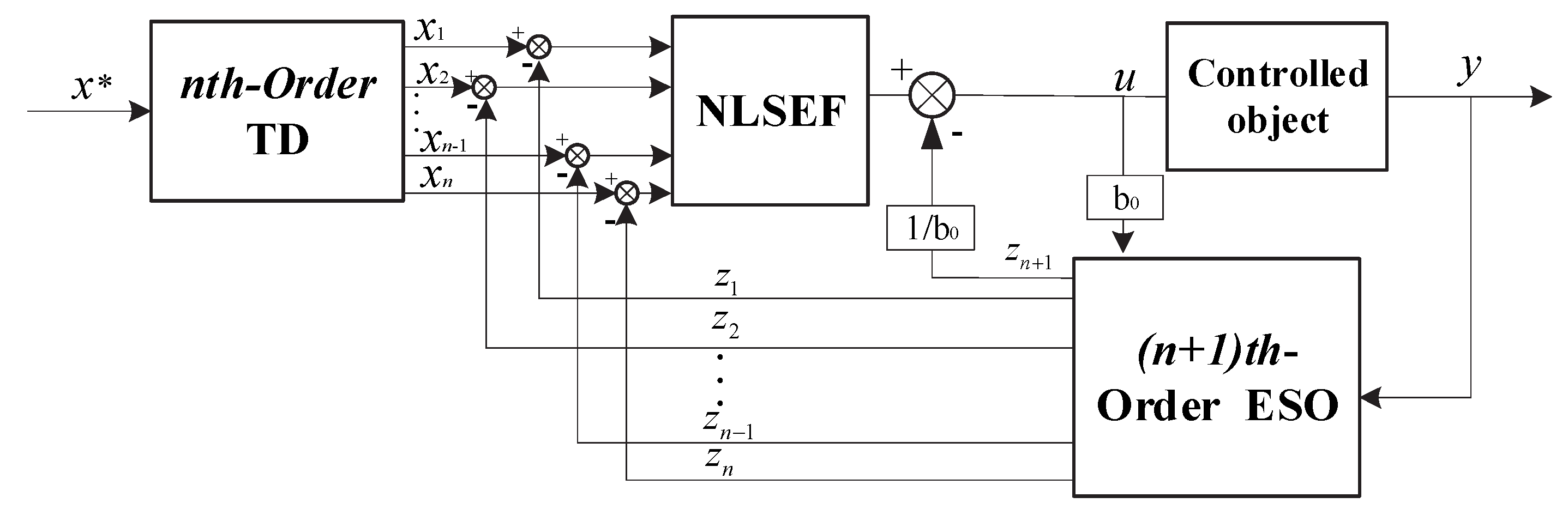
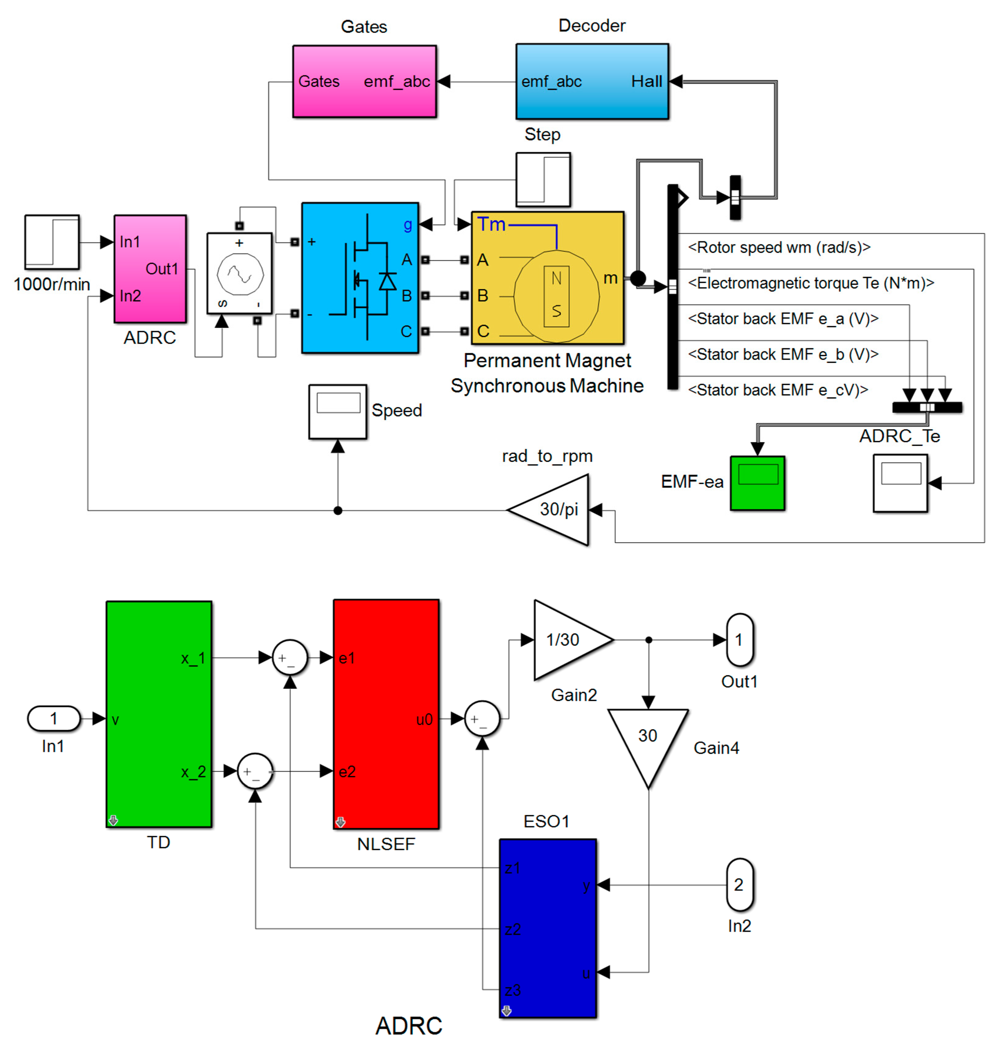
A schematic block diagram of the ADRC structure is shown in Figure 2. x* represents the input signal.
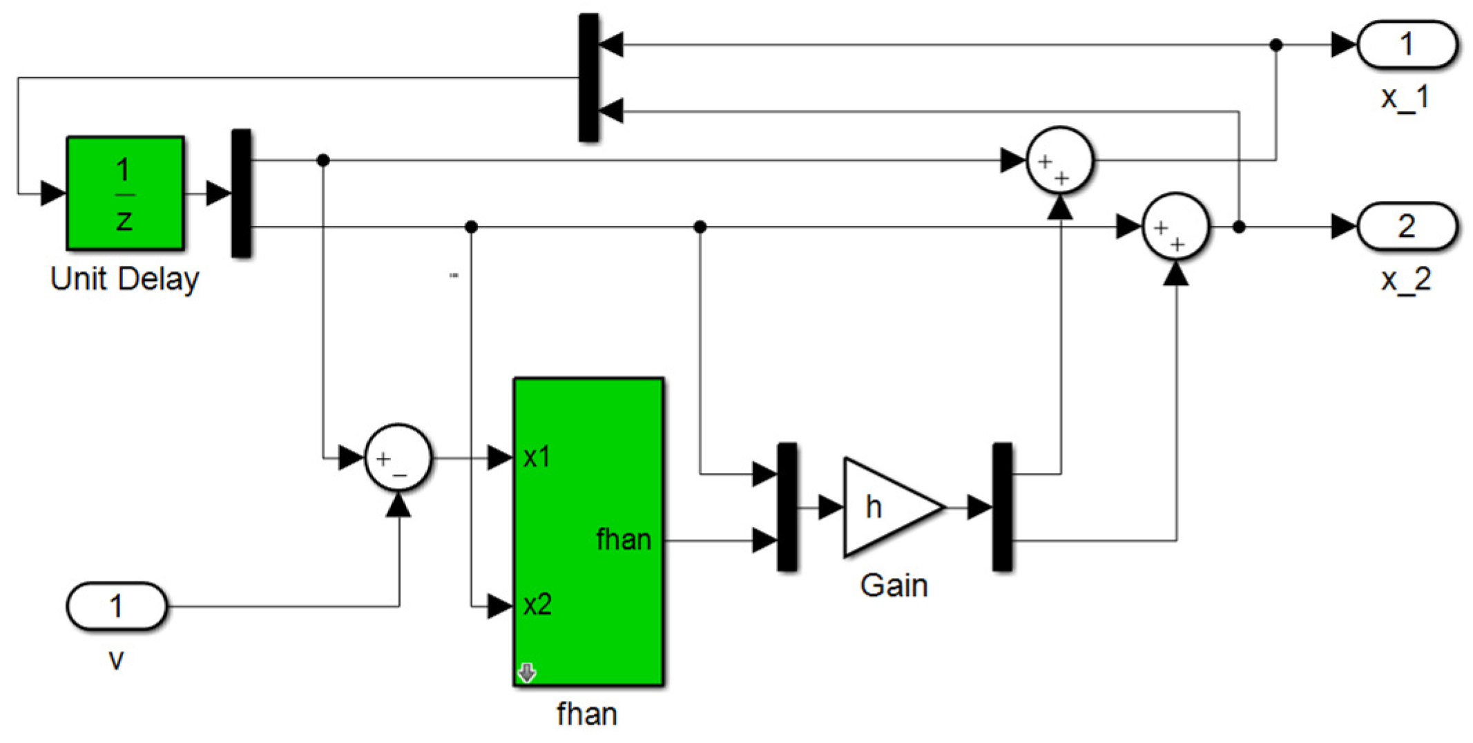
In practical applications, first-order ADRC and second-order ADRC are commonly utilized. Third- and higher-order ADRC expressions, which are complex and computationally intensive, necessitate higher controller performance and are less frequently employed. A typical differentiator replaces differentiation with differential approximation, as expressed:
v ˙ ( t ) = 1 h ( v ( t ) v ( t h ) )
When v(t) is contaminated by a noise signal, the use of differential computation amplifies the noise signal and may even overwhelm the differential signal. h is the sampling period. To address this issue, Jingqing Han proposed tracking the input signal using TD and obtaining the differential signal by solving the differential equations and using the integration result.
TD can smoothly track input signals, especially when the input signal contains noise or discontinuity. The tracking differentiator can convert these signals into continuous and smooth signals, thus avoiding the problems that may arise from direct step changes. Second, tracking differentiators can extract the differentiation of signals, which is crucial for control systems that need to understand the rate of signal change. In addition, it can also be used to arrange the transition process so that the output signal can smoothly transition from the current state to the target state, avoiding the impact and instability caused by direct step changes.
This approach is represented by TD as follows:
x 1 ( k + 1 ) = x 1 ( k ) + h x 2 ( k ) x 2 ( k + 1 ) = x 2 ( k ) +                         h f h a n ( x 1 ( k ) x i n ( k ) , x 2 ( k ) , r , h 1 )
fhan(·) is the core component of TD, and its main function is to act as a buffer. fhan(·) can help the system achieve fast and stable tracking of target signals while avoiding overshooting and improving control performance. fhan(·) is the fastest integrating function, which is written as
f h a n ( ) = d = r h 1 ;                                   d 0 = h 1 d y = x 1 + h 1 ( x 2 v ( k ) ) ; a 0 = d 2 + 8 r y a = x 2 + ( a 0 d ) 2 ,   y > d 0 x 2 + y h 1 ,   y d 0 f s t = r a d ,   a d r s i g n ( a ) , a > d s i g n ( a ) = 1                                             a > 0 1                                       a < 0
TD ensures that x1 converges to the input signal xin, x2 is the differential signal x1, r is the speed factor, which determines the tracking speed, T is the integration step size, and h1 is the filter factor. In this case, a larger h1 reflects a more obvious filter effect.
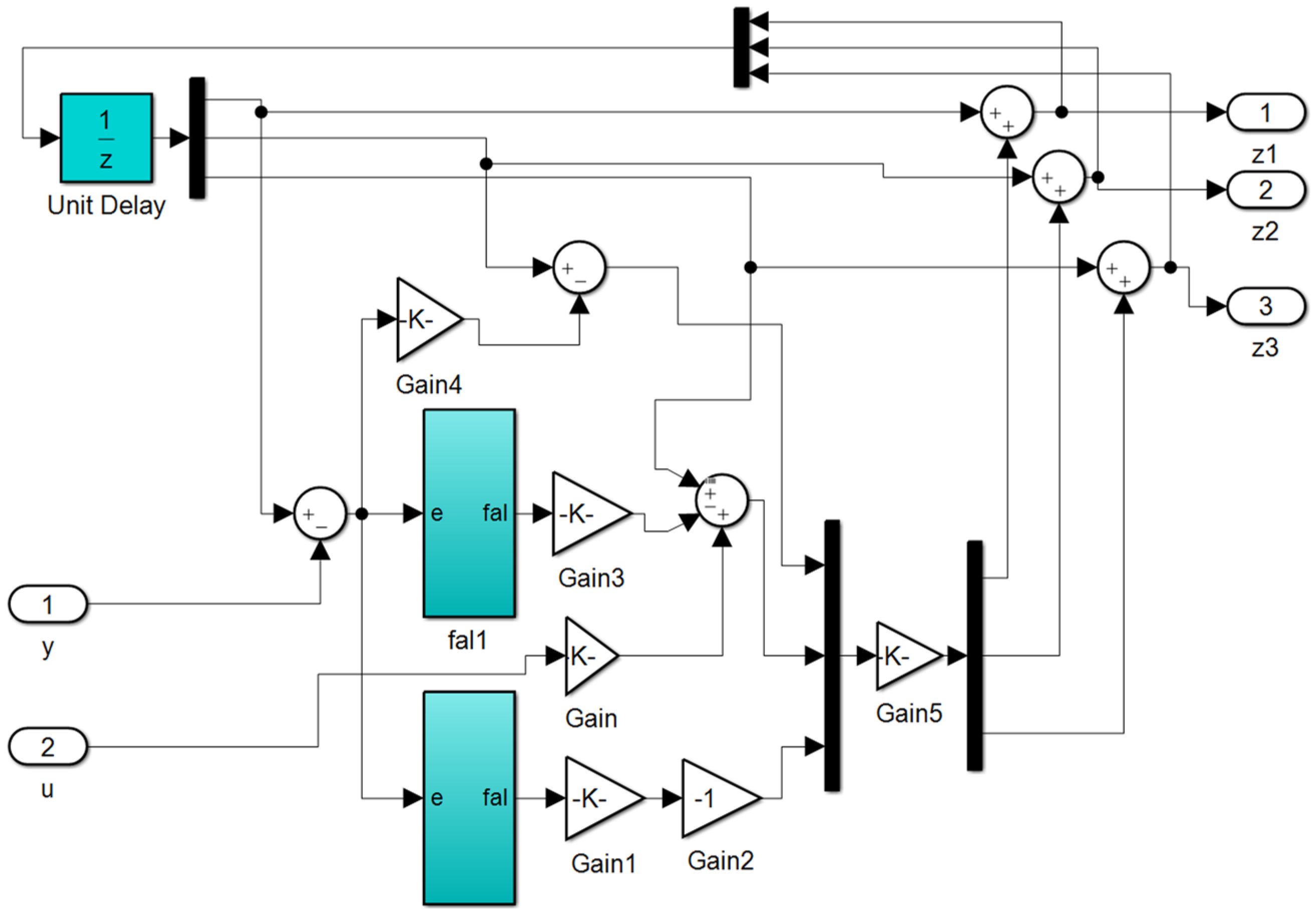
The primary role of the ESO is to monitor internal and external perturbations affecting the system’s output. The main concept of ESO involves expanding the total perturbation of the system into a new state variable higher than the first-order controlled object and then reconstructing the system’s original state variables and perturbations using inputs and outputs. For a second-order control object with a state equation
x ˙ 1 ( t ) = x 2 ( t ) x ˙ 2 ( t ) = f ( x 1 , x 2 , w ( t ) , t ) + b u ( t ) y = x 1 ( t )
w(t) is the external perturbation and f(x1, x2, w(t), t) represents the sum of the internal and external perturbations, or the “total perturbation”. As a new unknown state variable, x3(t) = f(x1, x2, w(t), t) expands a new state on the basis of Equation (14), and the original second-order state equation is expressed as follows:
x ˙ 1 ( t ) = x 2 ( t ) x ˙ 2 ( t ) = x 3 ( t ) + b u ( t ) x ˙ 3 ( t ) = f ˙ ( x 1 , x 2 , w ( t ) , t ) = w 0 ( t ) y = x 1 ( t )
The construction of a nonlinear state observer for Equation (15) has
e 1 = z 1 ( k ) y ( k ) z 1 ( k + 1 ) = z 1 ( k ) + h [ z 2 ( k ) β 01 e 1 ] z 2 ( k + 1 ) = z 2 ( k ) +                                         h [ z 3 ( k ) β 02 f a l ( e 1 , α 01 , δ ) + b u ] z 3 ( k + 1 ) = z 3 ( k ) h β 03 f a l ( e 1 , α 02 , δ )
β01, β02, and β03 are the output error correction gains. The β01, β02, and β03 values are related to the sampling period. where fal(·) is a nonlinear function written as
f a l ( x , α , δ ) = e δ 1 α                             e δ   s i g n ( e ) e α           e > δ  
where δ is an adjustable parameter, typically set to the same value as h. α01 and α02 generally take values of 0.5 and 0.25, respectively. The nonlinear ESO can be transformed into a linear ESO (LESO) by substituting fal() with e.
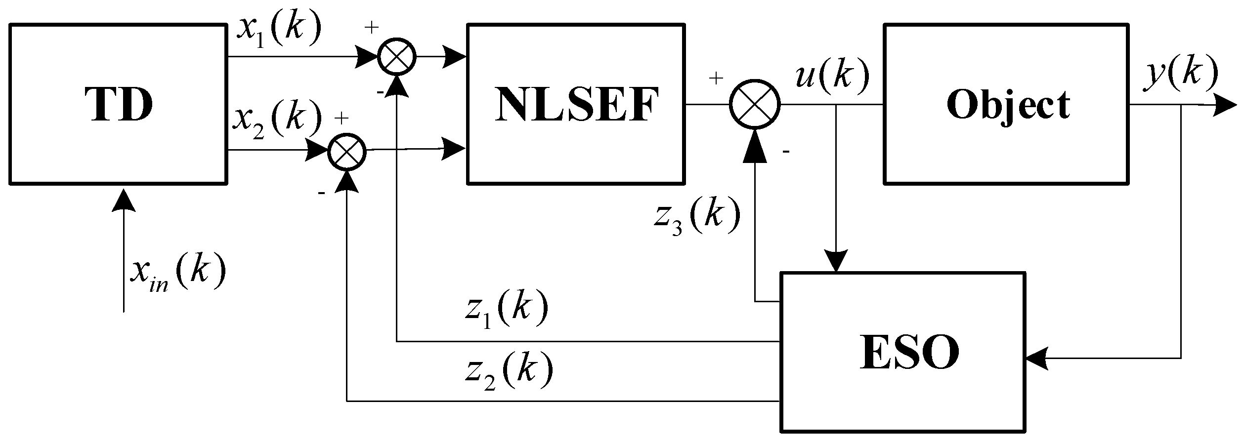
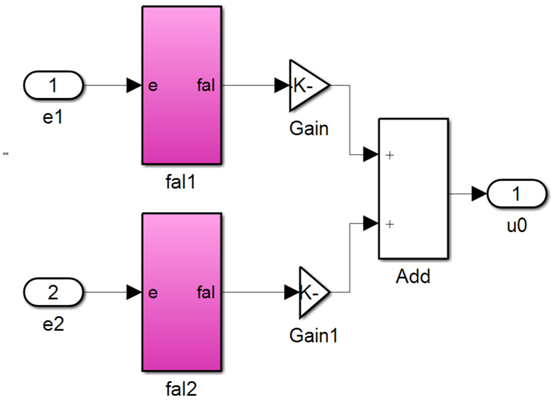
TD generates the error signal e1 and the differential signal of the error e2, and NLSEF replaces linear feedback in PID with non-smooth feedback of the error. NLSEF implements the digital adaptation of “small gain with large error, large gain with small error” through the fal(·) function. Variable gain PID, fuzzy control, and intelligent control all utilize this “small error, large gain; large error, small gain” control philosophy for regulation. The expression of the second-order NLSEF is shown in Equation (18).
e 1 = x 1 ( k ) z 1 ( k ) ,   e 2 = x 2 ( k ) z 2 ( k ) u 0 ( k ) = β 1 f a l ( e 1 , α 1 , δ ) + β 2 f a l ( e 2 , α 2 , δ ) u ( k ) = u 0 ( k ) z 3 ( k ) b 0
where 0 < α1 < 1 < α2, u0(k) becomes the PD output when fal(e1, α1, δ) = e1 and fal(e1, α1, δ) = e2. u(k) denotes the output of the system. β1 and β2 are the error gain and differential gain, respectively.
A block diagram of the control structure of the second-order ADRC is depicted in Figure 3.

3.2. Speed Loop Second-Order ADRC

In BLDC speed mode operation, the input to the TD is the target speed signal, and the input to the expanded observer is the speed signal from measurement feedback.
Let T1 = TL + Bω. Then,
J d ω d t = K t I s T 1
Differentiating Equation (19), we have
d 2 ω d t 2 = K t J d I s d t T ˙ 1 J
where wω(t) is the disturbance term, w ω ( t ) = 1 J [ T ˙ L + B d ω d t ] . The inputs to the second-order speed ADRC controller are the setpoint speed and the actual feedback speed. If the mechanical angular speed is ω1 and the angular acceleration is ω2, then
d ω 1 d t = ω 2 d ω 2 d t = d 2 ω 1 d t 2 = f ( ω 1 , ω 2 ) + w ω ( t ) + b 0 u
The expression for the second-order speed loop ADRC is shown in Equation (22):
ω ( k + 1 ) = ω ( k ) + T a ( k ) ω ( k + 1 ) = ω ( k ) +                         T f h a n ( ω ( k ) ω r e f , ω ( k ) , r 0 , h ) e = ω ( k ) y ( k ) ω ^ r ( k + 1 ) = ω ^ ( k ) + T ( a ^ ( k ) β 01 e ) a ^ ( k + 1 ) = a ^ ( k )           + T ( w ω ( k ) β 02 f a l ( e , 0.5 , δ ) + b 0 i q ( k ) ) w ω ( k + 1 ) = w ω ( k ) T β 03 f a l ( e , 0.5 , δ ) e 1 ( k ) = ω ( k ) ω ^ ( k ) e 2 ( k ) = a ( k ) a ^ ( k ) i ^ q ( k ) = β 1 f a l ( e 1 ( k ) , α 1 , δ )                                         + β 2 f a l ( e 2 ( k ) , α 2 , δ ) i q ( k ) = i ^ q ( k ) w ω ( k ) b 0
A block diagram of the ADRC-based BLDC speed control is shown in Figure 4.

4. Analysis of the Simulation Experiment Results

The ADRC-based BLDC six-step phase change method control model is constructed in the MATLAB/Simulink (2016b) environment. The target speed is set to 1000 r/min. After stabilizing the PMSM, a 4 Nm load is applied for 0.5 s to test the load disturbance resistance of both the PI-based and ADRC-based BLDC.
The parameters of the BLDC in the simulation model are shown in Table 1.
The system model is illustrated in Figure 5. In the ADRC, r = 3 × 10⁵, h = 5.5 × 10⁻⁶, β01 = 3 × 10⁶, β02 = 1 × 10⁴, β03 =1 × 10⁶, α1 = 0.5, α2 = 1.5, δ = 1, β1 = 2 × 10⁴, and β2 = 0.1. In the PI controller, kp = 1.5 and ki = 0.01.
The TD model in the ADRC is shown in Figure 6.
The ESO model in the ADRC is shown in Figure 7.
The NLSEF model in ADRC is shown in Figure 8.
As depicted in Figure 5, the input of the ADRC is the set speed and the feedback measured speed, and the output is the pulse width of the control PWM wave. By adjusting the pulse width of the PWM, the phase current can be adjusted, thereby controlling the motor torque. The decoder’s role in the model is to control and detect the motor rotor’s position. By measuring the Hall signal, the position and speed of the BLDC rotor can be accurately determined. The Hall signal is converted by the six-step commutator table and output to the Gates module, which drives the inverter. The decoder and the Gates module are shown in Figure 9 and Figure 10.
Setting the system simulation time to 0.5 s and the motor speed to 1000 r/min, a 4 Nm load is applied to the motor at 0.25 s, and the speed and torque changes of the BLDC are recorded. The speed change is shown in Figure 11. From the partially enlarged Figure A of Figure 11, it can be concluded that, given the 1000 r/min step signal, the time to reach 1000 r/min is the same for both the PI and ADRC control methods, at 0.01 s. However, the PI control method exhibits overshoot, with a maximum speed of 1036 r/min and an overshoot of 3.6%. The ADRC control method is capable of handling speed fluctuations after a 0.25 s load application. The speed fluctuation of the PI control mode is significantly larger than that of the ADRC control mode, as observed in the partially enlarged Figure 11B. The minimum speed fluctuation in the PI mode is 860 r/min, and the maximum is 1020 r/min, indicating that the load disturbance resistance of the PI mode is considerably weaker than that of the ADRC mode. After 0.28 s of stabilization, the speed fluctuation amplitude of the PI mode is significantly larger than that of the ADRC mode.
The error integral criterion is employed to evaluate the load disturbance resistance of the BLDC accurately using both the PID and ADRC methods.
This criterion is a comprehensive indicator that combines the magnitude of the error with the duration of its existence. The smaller the value of this criterion is, the better the system’s performance. According to the relevant literature [32,33,34,35], common performance indicators for control systems include ISE, ITSE, IAE, and ITAE. Each performance index focuses on different aspects of the system response. The ISE is the square integral of the error during the sampling time period of the system and is used to evaluate the stability of the system. The smaller the ISE is, the stronger the system stability. The ITSE criterion emphasizes reducing the error in the later stages of the transient response and is less sensitive to large initial errors. The IAE criterion is independent of time-integrated errors and provides appropriate damping and excellent transient response characteristics. However, it does not respond significantly to system parameter changes. The ITAE criterion offers advantages such as fast response speed, minimal oscillation, and effective control parameter selection. It is often considered the preferred performance evaluation index for single-input–output and adaptive systems. The expressions for ISE, ITSE, IAE, and ITAE are provided in Equation (23).
ISE = 0 e 2 ( t ) d t ITSE = 0 t e 2 ( t ) d t IAE = 0 e ( t ) d t ITAE = 0 t e ( t ) d t
The time period from 0.25 to 0.3 s was selected for calculating the four error integration criteria using the relative time approach. The results are presented in Table 2.
From these results, it is evident that the ADRC method outperforms the PI method in all four error criteria, with a notably smaller ITAE. This finding suggests that ADRC has superior load disturbance resistance compared to the PI method.
The variation in torque during the starting and loading processes is shown in Figure 12. The simulation results reveal that at approximately 0.02 s, the torque under PI control exhibits significant fluctuations, consistent with the speed fluctuations observed in Figure 11. After applying a 4 Nm load at 0.25 s, the torques for both the PI and ADRC control methods increase from 0 Nm to 4 Nm. After stabilizing at 0.3 s, the torque fluctuation amplitude under PI control is larger than that under ADRC control.
The current variation curve during speed operation is shown in Figure 13. The change in current is consistent with the change in torque. During operation from 0.02 to 0.05 s, the torque amplitude of the PI control method fluctuates significantly, and the corresponding current amplitude of the PI control method also fluctuates significantly. During stable operation from 0.3 s to 0.5 s, the current fluctuation amplitude of the PI control mode is greater than that of the ADRC control mode, and the corresponding torque fluctuation amplitude is also greater than that of the ADRC control mode.
The operating conditions were set to the same speed but different loads, the target speed was set to 1000 r/min, and a load of 6 Nm was applied at 0.25 s. The simulation results of the speed and torque are shown in Figure 14. The simulation variation patterns of the speed and torque are the same as those in Figure 11 and Figure 12.
The operating conditions were set at different speeds and loads, with an initial speed of 500 r/min. A 4 Nm load is applied at 0.2 s, and an additional 2 Nm load is applied at 0.3 s, with a load of 6 Nm. The load is set to 0 at 0.4 s. The target speed is set to 1000 r/min at 0.5 s, a 4 Nm load is applied at 0.6 s, another 2 Nm load is added at 0.7 s, and the load is 6 Nm at this time. The load is set to 4 Nm at 0.8 s. The speed simulation results of this process are shown in Figure 15. From the speed simulation results, it can be concluded that the ADRC control method has better resistance to load disturbances than the PI control method at different speeds.
The torque simulation results of this process are shown in Figure 16. From the torque simulation results, it can be concluded that after loading for 0.2 s, 0.3 s, 0.6 s, and 0.7 s, both the PI control method and ADRC control method can achieve the set target load, and the torque fluctuation amplitude of ADRC control is smaller than that of PI control.

5. Analysis of the Experimental Results

To validate the effectiveness of the ADRC-based BLDC control method, experimental verification was conducted using the STM32F4 control platform. The STM32F4 controller (STMicroelectronics, Geneva, Switzerland), known for its fast computing speed and low power consumption, integrates DSP instructions and a floating-point unit, making it well-suited for complex control algorithms such as ADRC. The experimental setup is illustrated in Figure 17, with the BLDC connected to a load brake using rigid coupling. During the experiment, a magnetic particle brake applies the load to the BLDC, and the STM32 controller sends speed data to the host computer at 10 ms intervals.
The parameters of the BLDC and magnetic powder brake used in the experiments are shown in Table 3.
The system sampling time is 10 ms. For the ADRC, r = 8000, h = 0.015, β01 = 15.6, β02 = 780, β03 = 1010, α1 = 0.75, α2 = 1.75, δ = 1, β1 = 280.1, and β2 = 130.1. In the PI controller, kp = 0.035 and ki = 0.02.
The flowchart of the control algorithm is shown in Figure 18. STM32’s advanced timers 1 and 8 have a three-phase Hall signal acquisition function. The rotation direction and speed of the BLDC are determined by detecting Hall signals. The calculated speed signal is sent to the PI/ADRC controller, which adjusts the duty cycle of the PWM output to change the BLDC’s speed.
During the experiment, the BLDC was set to rotate at 1000 r/min and 1500 r/min. The load was applied and then removed after speed stabilization, and the speed change data were recorded and plotted.
To adjust the control parameters of the ADRC and PID controllers, the speed was set to 1000 r/min. After stabilizing the speed, a 0.1 Nm load was applied to the BLDC at 3.00 s and then removed at 5.00 s after the speed returned to 1000 r/min. The resulting speed change curve is shown in Figure 19.
From the local magnification in Figure 18, it is evident that both the ADRC and PID control methods can maintain a steady state at 1000 r/min, with the same steady-state error. However, the time taken to reach the target speed is 0.62 s for both methods. The PI control mode exhibits overshoot, with a peak speed of 1018 r/min and an overshoot of 1.8%. During loading and unloading, the PID control method shows a larger fluctuation amplitude in speed than the ADRC method. The minimum speed for PID control during loading is 841 r/min, while it is 940 r/min for ADRC control. During unloading, the maximum speed for PID control is 1180 r/min, compared to 1068 r/min for ADRC control.
Using the relative time method, the speed changes during loading and unloading were analyzed, and the resulting speed change curve is depicted in Figure 20. From Figure 20, it is inferred that the rotational speed changes during loading and unloading are opposite in nature and almost symmetrical. The convergence speed of ADRC is faster than that of the PID control method.
Given the symmetrical nature of the speed changes in the two control modes, PID and ADRC, during the loading and unloading processes, the study utilizes speed data from the loading process only for the quantitative analysis of disturbance performance in the ADRC and PID control modes. The selected time period for analysis ranged from 3.00 to 4.00 s, and the relative time method was used to calculate four error integration criteria. The results of these calculations are presented in Table 4.
The data in Table 4 indicate that at 1000 r/min operation, the ADRC control mode demonstrates superior performance in all four error integration criteria compared to the PID control mode, highlighting its enhanced stability during both the loading and unloading processes.
The speed is set at 1500 r/min, and upon stabilization, a 0.1 Nm load is applied to the BLDC at 3.00 s. After the speed returns to 1000 r/min, the load is removed at 5.00 s. The resulting speed variation curve is illustrated in Figure 21. A detailed examination of Figure 17 reveals that both systems achieve 1500 r/min in an identical duration of 1.00 s and maintain the same steady-state error thereafter. During the loading phase, the minimum speed reached by the PID control mode is 1295 r/min, while for the ADRC control mode, it is 1420 r/min. Similarly, during unloading, the maximum speed for the PID control mode is 1730 r/min, compared to 1589 r/min for the ADRC mode, with target speeds of 1500 r/min and 1000 r/min for loading and unloading, respectively. This pattern of speed change is consistent across both modes.
By applying the relative time method, the speed variation curve at 1500 r/min during loading and unloading is depicted in Figure 22. This figure shows that the rotational speed change during these processes is essentially symmetrical. The ADRC control method converges to 1500 r/min at 0.8 s, faster than the PID control method, which achieves the same speed at 1000 r/min.
As the speed changes of the PID and ADRC control methods during loading and unloading are essentially symmetrical, only the loading process speed data are used for the quantitative disturbance control performance analysis of ADRC and PID. The chosen analysis period is from 3.00 to 4.00 s, and the relative time method is used to calculate the four error integration criteria at a loading speed of 1500 r/min. The results are displayed in Table 5.
Table 5 shows that at 1500 r/min, the ADRC control mode’s performance in terms of the four error integration criteria surpasses that of the PID control mode, indicating more effective disturbance control during both the loading and unloading processes.
The speed is set at 1500 r/min, and upon stabilization, a 0.2 Nm load is applied to the BLDC at 3.00 s. After the speed returns to 1500 r/min, the load is removed at 5.00 s. The resulting speed variation curve is illustrated in Figure 23. The minimum speed of the PI control mode during loading is 1139 r/min, and the minimum speed of the ADRC control mode during loading is 1330 r/min. The maximum speed of the PI control mode during unloading is 1917 r/min, and the maximum speed of the ADRC control mode during unloading is 1689 r/min.
The speed variation curve at 1500 r/min during the loading and unloading process is shown in Figure 24. The changes in speed during these processes are basically symmetrical. The speed variation pattern during the loading and unloading process is consistent with Figure 21.
The chosen analysis period is from 3.00 to 4.00 s, and the relative time method is used to calculate the four error integration criteria at a loading speed of 1500 r/min. The results are displayed in Table 6.

6. Conclusions

This paper proposes a six-step phase-change control method for BLDC based on ADRC. Mathematical models for BLDC and second-order ADRC are constructed, and the BLDC speed loop’s second-order ADRC mathematical expression is derived. This study provides an analytical method to quantitatively evaluate the resistance to load disturbances using four error integration criteria: the ISE, ITSE, IAE, and ITAE. A BLDC simulation model based on ADRC is established, analyzing the speed change rule of both the PI and ADRC control methods using a speed step signal of 1000 r/min. The resistance to load disturbances using the PI and ADRC controllers is quantitatively analyzed. After applying a 4 Nm load, the ITAE for PI and ADRC are calculated as 2.08 × 10⁸ and 4.29 × 10², respectively. The method is then applied to the STM32F4 controller for experimental validation by conducting a detailed comparative analysis of the PI and ADRC control methods under operating conditions of 1000 r/min and 1500 r/min using the error integration criterion. The ITAE calculations for PI and ADRC at 1000 r/min are 1.77 × 10³ and 5.87 × 10², respectively, and at 1500 r/min, they are 3.36 × 10³ and 7.62 × 10², respectively. Both the simulation and experimental results demonstrate the superior load disturbance resistance of the ADRC compared to that of the STM32F4 controller.

Author Contributions

Conceptualization, P.Z. and H.Q.; methodology, P.Z. and B.Y.; software, P.Z.; validation, P.Z.; formal analysis, P.Z.; investigation, P.Z. and H.Q.; resources, Z.S.; data curation, P.Z.; writing—original draft preparation, P.Z.; writing—review and editing, P.Z. and H.Q.; visualization, P.Z.; supervision, H.Q.; project administration, Z.S.; funding acquisition, Z.S. All authors have read and agreed to the published version of the manuscript.

Funding

This research was funded by the National Natural Science Foundation of China Youth Fund (Granted No. 52305046).

Institutional Review Board Statement

Not applicable.

Informed Consent Statement

Not applicable.

Data Availability Statement

Data are contained within the article.

Conflicts of Interest

The authors declare no potential conflicts of interest with respect to the research, authorship, and publication of this article.

References

  1. Yedamale, P. Brushless DC (BLDC) motor fundamentals. Microchip Technol. Inc. 2003, 20, 3–15. [Google Scholar]
  2. Kim, T.H.; Ehsani, M. Sensorless control of the BLDC motors from near-zero to high speeds. IEEE Trans. Power Electron. 2004, 19, 1635–1645. [Google Scholar] [CrossRef]
  3. Nadolski, R.; Ludwinek, K.; Staszak, J.; Jaśkiewicz, M. Utilization of BLDC motor in electrical vehicles. Prz. Elektrotech. 2012, 88, 180–186. [Google Scholar]
  4. Low, T.S.; Lee, T.H.; Tseng, K.J.; Lock, K.S. Servo performance of a BLDC drive with instantaneous torque control. IEEE Trans. Ind. Appl. 1992, 28, 455–462. [Google Scholar] [CrossRef]
  5. Alphonse, I.; Thilagar, H.; Singh, F.B. Design of solar powered BLDC motor driven electric vehicle. Int. J. Renew. Energy Res. 2012, 2, 456–462. [Google Scholar]
  6. Carvajal, J.; Chen, G.; Ogmen, H. Fuzzy PID controller: Design, performance evaluation, and stability analysis. Inf. Sci. 2000, 123, 249–270. [Google Scholar] [CrossRef]
  7. Huang, G.; Yuan, X.; Shi, K.; Wu, X. A BP-PID controller-based multi-model control system for lateral stability of distributed drive electric vehicle. J. Frankl. Inst. 2019, 356, 7290–7311. [Google Scholar] [CrossRef]
  8. Pei, G.; Yu, M.; Xu, Y.; Ma, C.; Lai, H.; Chen, F.; Lin, H. An improved PID controller for the compliant constant-force actuator based on BP neural network and smith predictor. Appl. Sci. 2021, 11, 2685. [Google Scholar] [CrossRef]
  9. Ahn, K.K.; Truong, D.Q. Online tuning fuzzy PID controller using robust extended Kalman filter. J. Process Control 2009, 19, 1011–1023. [Google Scholar] [CrossRef]
  10. Dey, C.; Mudi, R.K. An improved auto-tuning scheme for PID controllers. ISA Trans. 2009, 48, 396–409. [Google Scholar] [CrossRef] [PubMed]
  11. Maji, T.K.; Acharjee, P. Multiple solutions of optimal PMU placement using exponential binary PSO algorithm for smart grid applications. IEEE Trans. Ind. Appl. 2017, 53, 2550–2559. [Google Scholar] [CrossRef]
  12. Maghfiroh, H.; Ramelan, A.; Adriyanto, F. Fuzzy-PID in BLDC motor speed control using MATLAB/Simulink. J. Robot. Control. (JRC) 2022, 3, 8–13. [Google Scholar] [CrossRef]
  13. Nasri, M.; Nezamabadi-Pour, H.; Maghfoori, M. A PSO-based optimum design of PID controller for a linear brushless DC motor. World Acad. Sci. Eng. Technol. 2007, 26, 211–215. [Google Scholar]
  14. Gupta, R.A.; Kumar, R.; Bansal, A.K. Artificial intelligence application in Permanent Magnet Brushless DC motor drives. Artif. Intell. Rev. 2010, 33, 175–186. [Google Scholar] [CrossRef]
  15. Mousmi, A.; Abbou, A.; El Houm, Y. Real-time implementation of a novel hybrid fuzzy sliding mode control of a BLDC motor. Int. J. Power Electron. Drive Syst. 2019, 10, 1167. [Google Scholar] [CrossRef]
  16. KMA, P.; Nair, U. Intelligent fuzzy sliding mode controller based on FPGA for the speed control of a BLDC motor. Int. J. Power Electron. Drive Syst. 2020, 11, 477. [Google Scholar]
  17. Wu, Z.; Gao, Z.; Li, D.; Chen, Y.; Liu, Y. On transitioning from PID to ADRC in thermal power plants. Control. Theory Technol. 2021, 19, 3–18. [Google Scholar] [CrossRef]
  18. Fareh, R.; Khadraoui, S.; Abdallah, M.Y.; Baziyad, M.; Bettayeb, M. Active disturbance rejection control for robotic systems: A review. Mechatronics 2021, 80, 102671. [Google Scholar] [CrossRef]
  19. Castañeda, L.A.; Luviano-Juárez, A.; Ochoa-Ortega, G.; Chairez, I. Tracking control of uncertain time delay systems: An ADRC approach. Control Eng. Pract. 2018, 78, 97–104. [Google Scholar] [CrossRef]
  20. Hezzi, A.; Ben Elghali, S.; Bensalem, Y.; Zhou, Z.; Benbouzid, M.; Abdelkrim, M.N. ADRC-based robust and resilient control of a 5-phase PMSM driven electric vehicle. Machines 2020, 8, 17. [Google Scholar] [CrossRef]
  21. Li, W.; Zhang, Q.; Zhang, Y. The effect of ADRC on vehicle braking performance. J. Electr. Eng. Technol. 2020, 15, 705–712. [Google Scholar] [CrossRef]
  22. Lotufo, M.A.; Colangelo, L.; Perez-Montenegro, C.; Canuto, E.; Novara, C. UAV quadrotor attitude control: An ADRC-EMC combined approach. Control Eng. Pract. 2019, 84, 13–22. [Google Scholar] [CrossRef]
  23. Zhang, Y.; Chen, Z.; Zhang, X.; Sun, Q.; Sun, M. A novel control scheme for quadrotor UAV based upon active disturbance rejection control. Aerosp. Sci. Technol. 2018, 79, 601–609. [Google Scholar] [CrossRef]
  24. Zhong, S.; Huang, Y.; Chen, S.; Dai, L. A novel ADRC-based design for a kind of flexible aerocraft. Control Theory Technol. 2021, 19, 35–48. [Google Scholar] [CrossRef]
  25. Krawczyk, M.; Zajdel, A. Automatic taxi directional control system for general aviation aircraft. J. Kones 2018, 25, 299–306. [Google Scholar]
  26. He, J.; Yan, C.; Wang, X. Torque ripple suppression of brushless DC motor drive system based on improved harmonic injection active disturbance rejection control. Sensors 2022, 22, 1069. [Google Scholar] [CrossRef]
  27. Chang, X.; Li, Y.; Zhang, W.; Wang, N.; Xue, W. Active disturbance rejection control for a flywheel energy storage system. IEEE Trans. Ind. Electron. 2014, 62, 991–1001. [Google Scholar] [CrossRef]
  28. Li, J.; Ren, H.P.; Zhong, Y.R. Robust speed control of induction motor drives using first-order auto-disturbance rejection controllers. IEEE Trans. Ind. Appl. 2014, 51, 712–720. [Google Scholar] [CrossRef]
  29. De la Guerra, A.; Alvarez-Icaza, L. Robust control of the brushless dc motor with variable torque load for automotive applications. Electr. Power Compon. Syst. 2020, 48, 117–127. [Google Scholar] [CrossRef]
  30. Liu, Z.; Liu, B.F. Robust control strategy for the speed control of brushless DC motor. J. Harbin Inst. Technol. 2013, 2, 90–94. [Google Scholar]
  31. Curiel-Olivares, G.; Linares-Flores, J.; Guerrero-Castellanos, J.F.; Hernández-Méndez, A. Self-balancing based on active disturbance rejection controller for the two-in-wheeled electric vehicle, experimental results. Mechatronics 2021, 76, 102552. [Google Scholar] [CrossRef]
  32. Hadi, N.H.; Ibraheem, I.K. Speed control of an SPMSM using a tracking differentiator-PID controller scheme with a genetic algorithm. Int. J. Electr. Comput. Eng. 2021, 11, 1728. [Google Scholar] [CrossRef]
  33. Khanh, P.Q.; Anh, H.P.H. Hybrid optimal fuzzy Jaya technique for advanced PMSM driving control. Electr. Eng. 2023, 105, 3629–3646. [Google Scholar] [CrossRef]
  34. Yun, H.M.; Kim, Y.; Choi, H.H. Differential evolution approach for performance enhancement of field-oriented PMSMs. J. Electr. Eng. Technol. 2018, 13, 2301–2309. [Google Scholar]
  35. Toloue, S.F.; Kamali, S.H.; Moallem, M. Multivariable sliding-mode extremum seeking PI tuning for current control of a PMSM. IET Electr. Power Appl. 2020, 14, 348–356. [Google Scholar] [CrossRef]
Figure 1. BLDC-equivalent circuit diagram.
Machines 12 00244 g001
Figure 2. Block diagram of the n-order ADRC control structure.
Machines 12 00244 g002
Figure 3. Block diagram of second-order ADRC.
Machines 12 00244 g003
Figure 4. Block diagram of ADRC sensor-less control.
Machines 12 00244 g004
Figure 5. System simulation model.
Machines 12 00244 g005
Figure 6. TD simulation model.
Machines 12 00244 g006
Figure 7. ESO simulation model.
Machines 12 00244 g007
Figure 8. NLSEF simulation model.
Machines 12 00244 g008
Figure 9. Decoder module.
Machines 12 00244 g009
Figure 10. Gates Module.
Machines 12 00244 g010
Figure 11. Speed simulation results.
Machines 12 00244 g011
Figure 12. Torque simulation results.
Machines 12 00244 g012
Figure 13. Current simulation results.
Machines 12 00244 g013
Figure 14. Speed and torque simulation results.
Machines 12 00244 g014
Figure 15. Simulation results for different speeds and torques.
Machines 12 00244 g015
Figure 16. Different torque simulation results.
Machines 12 00244 g016
Figure 17. Experimental platform.
Machines 12 00244 g017
Figure 18. Flowchart of the program.
Machines 12 00244 g018
Figure 19. Results of the 1000 r/min speed change test.
Machines 12 00244 g019
Figure 20. Speed change during loading and unloading at 1000 r/min.
Machines 12 00244 g020
Figure 21. 1500 r/min speed change test results.
Machines 12 00244 g021
Figure 22. The loading and unloading process speed changes at 1500 r/min.
Machines 12 00244 g022
Figure 23. The results of the variable speed test with a load of 0.2 Nm at 1500 rpm.
Machines 12 00244 g023
Figure 24. The loading and unloading process speed changes at 1500 r/min and 0.2 Nm, respectively.
Machines 12 00244 g024
Table 1. Simulation model parameters for BLDC.
NameValueNameValue
Number of phases3Inertia (kg.m2)8 × 10⁻⁴
Rs (Ω)0.7Inductance (H)2.72 × 10⁻³
Flux (V.s)0.105Pole pairs4
Table 2. Integral calculation results for errors within 0.2 to 0.3 s at 1000 r/min.
Control MethodISEITSEIAEITAE
PI2.08 × 1081.12 × 1062.35 × 1061.94 × 104
ADRC1.79 × 1055.42 × 1025.58 × 1044.29 × 102
Table 3. The parameters of BLDC.
NameValueNameValue
Rate Voltage (V)24No-load Speed (r/min)3500
Rate Current (A)5.9Rate Torque (Nm)0.38
Rate Speed (r/min)2500Pole pairs4
Brake output torque (Nm)1.5Brake Voltage (V)24
Table 4. Integral calculation results of 3 to 4s error under a load condition of 1000 r/min and 0.1 Nm.
Control MethodISEITSEIAEITAE
PI7.01 × 1051.71 × 1056.14 × 1031.77 × 103
ADRC8.98 × 1041.91 × 1042.17 × 1035.87 × 102
Table 5. Integral calculation results of 3 to 4s error under a load condition of 1500 r/min and 0.1 Nm.
Control MethodISEITSEIAEITAE
PI1.42 × 1063.98 × 1059.85 × 1033.36 × 103
ADRC1.54 × 1053.17 × 1042.88 × 1037.62 × 102
Table 6. Integral calculation results of 3 to 4s error under a load condition of 1500 r/min and 0.2 Nm.
Control MethodISEITSEIAEITAE
PI4.72 × 1061.51 × 1061.85 × 1047.17 × 103
ADRC8.94 × 1052.13 × 1057.37 × 1032.21 × 103
Disclaimer/Publisher’s Note: The statements, opinions and data contained in all publications are solely those of the individual author(s) and contributor(s) and not of MDPI and/or the editor(s). MDPI and/or the editor(s) disclaim responsibility for any injury to people or property resulting from any ideas, methods, instructions or products referred to in the content.

