Milling Tool Wear Monitoring via the Multichannel Cutting Force Coefficients

Abstract

Tool wear monitoring (TWM) is of great importance for improving the machining quality and the efficiency of the milling process. Extracting a discriminative tool wear feature is the key to TWM. Cutting force coefficients, which reflect the tool–chip and tool–material contact form, are good indicators of tool wear condition. However, in the existing studies, only the tangential and radial cutting force coefficients are adopted to monitor tool wear. The axial coefficients extracted from the axial cutting force are neglected. Preliminary experiments have shown that, although the axial cutting force has a small amplitude, the axial cutting force coefficients are very discriminative regarding the tool wear condition. Fusing the axial coefficients and the traditional tangential and radial coefficients can improve the monitoring accuracy. Based on such a consideration, this study proposes a milling tool wear monitoring method in which the multichannel cutting force coefficients, viz., the tangential, radial, and axial cutting force coefficients, are fused to indicate the tool wear. A long short-term memory (LSTM) network is adopted to sequentially estimate the progressive tool wear value from the multichannel cutting force coefficients. The effectiveness of the proposed monitoring method is examined using the PHM 2010 data. The results show that the proposed method outperforms the traditional method. With the fusion of the multichannel coefficients, the monitoring accuracy improves by 2.74–6.35%.

1. Introduction

Tool wear decreases the machining quality and the efficiency of the milling process. Severe tool wear will even cause tool breakage and destroy the workpiece and the machine [1]. According to statistics, the downtime caused by tool wear failure accounts for 20% of the total working hours, and the related economic loss accounts for 15–40% of the total cost [2]. The tool wear monitoring system, which can make an accurate online estimation of tool wear and provide an alert regarding tool failure, is of great importance for improving the machining quality and efficiency [3].

Online assessments of tool wear are usually conducted by inferring the tool wear from the monitoring signals [4]. Commonly used monitoring signals are cutting force [5,6], vibration [7], acoustic emission [8], and rotor current [9]. Because of its ability to sense tool wear condition, the cutting force signal has been widely adopted in tool wear monitoring systems. However, due to the high sampling rate of the cutting force signal generated in the milling process, the cutting force data are excessive and redundant. It is not proper to estimate the tool wear from the raw cutting force signal. Extracting low-dimensional and discriminative tool wear features is necessary for constructing an efficient tool monitoring system for the milling process.

The cutting force coefficient, which represents the force distribution in the tool–chip and tool–material contact zones, has proven to be a discriminative tool wear feature [10,11]. From a modeling perspective, the cutting force coefficients can be regarded as parameters of the model representing the relationship between the uncut chip thickness and cutting force. Therefore, the cutting force coefficients can be extracted by identifying the model. In recent years, the milling force model has been deeply investigated, leading to a good theoretical foundation for model identification and cutting force coefficient extraction [12,13]. In the study of milling titanium alloys, Lu et al. [14] accurately predicted the micro-milling cutting force under the tool wear state by establishing a mapping relationship between the flank wear and cutting force. Zhou et al. [15] comprehensively considered the effects of the radius of the cutting edge on the shear/plowing force coefficient and the wear width of the flank face on the friction coefficient and established a milling cutting force model that includes both cutting edge wear and flank wear. Nouri et al. [16] built a dual cutting force coefficient model to represent the relationship between UCT and cutting force and extracted the cutting force coefficient from the cutting force signal to monitor the tool wear. Hou et al. [17] built an analytic force model considered flank tool wear and calculated the flank wear from the friction force coefficient in the flank wear region. Pan et al. [18] adopted the cutting parameter-independent coefficients that were extracted from the mechanistic cutting force model to estimate the tool wear. Liu et al. [19] extracted the cutting parameters and tool runout-independent cutting force coefficients to estimate the tool wear under variable cutting parameters and runout in the micro-milling process.

The adopted cutting force coefficients in the studies mentioned above were mainly the coefficients that were extracted from the tangential and radial cutting forces. Because the amplitude of the axial cutting force in the milling process is small, the axial coefficients corresponding to the axial force wear are usually neglected in tool wear monitoring. In this study, it was considered that although the axial force is small, the axial coefficients are sensitive to the tool wear condition, and incorporating the axial coefficients into the monitoring system must improve the monitoring accuracy. Based on such a consideration, this study proposes a milling tool wear monitoring method in which the multichannel cutting force coefficients, viz., the tangential, radial, and axial cutting force coefficients, are fused to indicate the tool wear. The long short-term memory network is adopted to sequentially estimate the progressive tool wear value from the multichannel cutting force coefficients. The effectiveness of the proposed monitoring method is examined via the PHM 2010 data.

This study evolves as follows. The cutting force model and the extraction of the cutting force coefficients are presented in Section 2. The tool wear monitoring is conducted in Section 3. The effectiveness of the proposed monitoring method is validated in Section 4. The study is concluded in Section 5.

2. Cutting Force Model and Cutting Force Coefficient Extraction

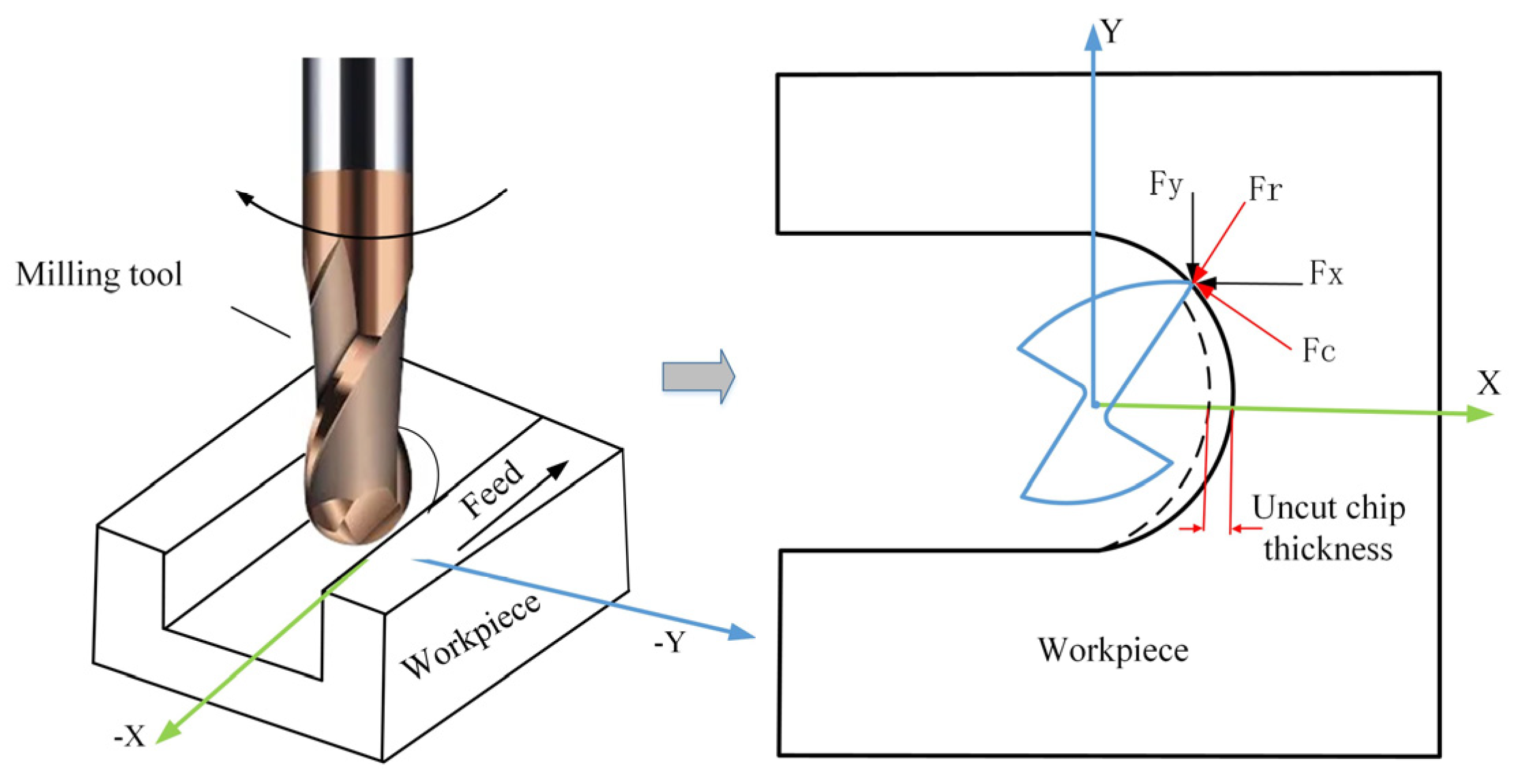
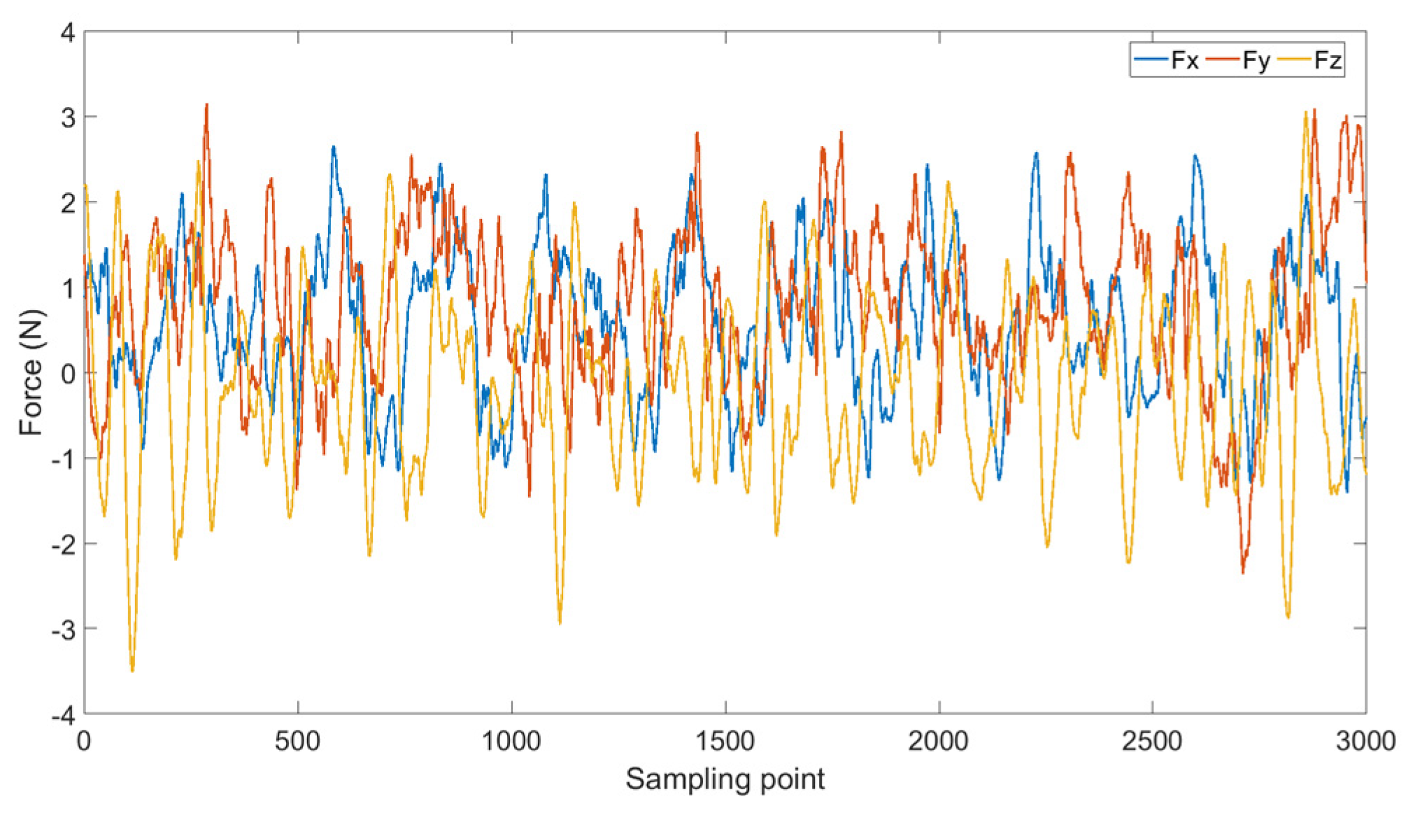
2.1. Mechanistic Cutting Force Model for the Milling Process

Equations (1)–(3) mathematically describe the mechanistic cutting force model parameterized by the cutting force coefficients. As the equations show, the model represents the relationship between the uncut chip thickness and cutting force.

$$F_c=\left(K_{c,sp}h+K_{c,vb}\right)d$$

(1)

$$F_r=\left(K_{r,sp}h+K_{r,vb}\right)d$$

(2)

$$F_a=\left(K_{a,sp}h+K_{a,vb}\right)d$$

(3)

where Fc is the tangential force, Fr is the radial force, Fa is the axial force, h is the instantaneous uncut chip thickness, d is the axial cutting depth, Kc,sp is the shear/ploughing coefficient in the tangential direction, Kr,sp is the shear/ploughing coefficient in the radial direction, Ka,sp is the shear/ploughing coefficient in the axial direction, Kc,vb is the friction force coefficient in the tangential direction, Kr,vb is the friction force coefficient in the radial direction, and Ka,vb is the friction force coefficient in the axial direction. The six cutting force coefficients were categorized into three classes in terms of direction: tangential, radial, and axial direction. In terms of the effecting mechanism, the six cutting force coefficients were categorized into two classes: the shear/ploughing coefficients and the friction force coefficients. The shear/ploughing coefficients correspond to the force distribution in the rake face and cutting-edge zone and thus reflect the wear condition of the rake face and cutting edge. The friction force coefficients correspond to the force distribution in the flank wear zone and thus reflect the flank wear condition. The six cutting force coefficients are listed in

Table 1. The multichannel cutting force coefficients.

	Shear/Ploughing	Friction in Flank Region
Tangential	Kc,sp (N/mm2)	Kc,vb (N/mm)
Radial	Kr,sp (N/mm2)	Kr,vb (N/mm)
Axial	Ka,sp (N/mm2)	Ka,vb (N/mm)

.

The uncut chip thickness periodically varies with the rotation angle, as Equation (4) shows.

$$h\left(\theta \right)=f_z\sin \left(\theta \right)$$

(4)

where $f_z$ is the feed per tooth. In practice, in precision milling, the uncut chip thickness also varies with tool runout parameters such as runout length and runout angle [20,21]. This study mainly considered the conventional milling process, which is less affected by the tool runout. Thus, the simplified form without considering the tool runout effect was adopted to mathematically represent the uncut chip thickness, as Equation (4) shows.

Compared to the tangential and radial forces, the forces in the feed and normal directions are easier to collect, as most commercial force meters use Cartesian coordinates. Instead of the tangential and radial forces, the tangential and radial coefficients are usually extracted from the cutting forces in the feed and normal directions. According to the decomposition form shown in Figure 1, the cutting forces in the feed and normal directions can be mathematically written as Equations (5) and (6).

$$F_x=\left[K_{c,sp}h\cos \left(\theta \right)+K_{c,vb}\cos \left(\theta \right)+K_{r,sp}h\sin \left(\theta \right)+K_{r,vb}\sin \left(\theta \right)\right]d$$

(5)

$$F_y=\left[K_{c,sp}h\sin \left(\theta \right)+K_{c,vb}\sin \left(\theta \right)-K_{r,sp}h\cos \left(\theta \right)-K_{r,vb}\cos \left(\theta \right)\right]d$$

(6)

2.2. Identification of the Multichannel Cutting Force Coefficients

The cutting force coefficients were extracted by identifying the cutting force model defined in Section 2.1. The input of the model is the instantaneous uncut chip thickness, and the output of the model is the cuttingforce. The cutting force coefficients are regarded as the model parameters to be identified. The identified coefficients are the model parameters that create an optimal fitting relationship between the measured cutting forces and the predefined uncut chip thickness. The measured feed and the radial and axial forces in a short cutting pass are denoted by vectors $F_x$, $F_y$, and $F_a$, and the predefined instantaneous uncut chip thickness in a short cutting pass is denoted by vector $h$. The four vectors involved in the identification process are defined as:

$$\begin{array}{l}hc:=h.\ast \cos \left(\theta \right)\\ c:=\cos \left(\theta \right)\\ hs:=h.\ast \sin \left(\theta \right)\\ s:=\sin \left(\theta \right)\end{array}$$

(7)

With the definitions of the four vectors, the cutting force model in Section 2.1 can be written in matrix form using Equation (8).

$$\left[\begin{array}{c}{F}_x/d\\ F_y/d\\ F_a/d\end{array}\right]=\left[\begin{array}{cccccc}hc& c& hs& s& 0& 0\\ hs& s& -hs& -c& 0& 0\\ 0& 0& 0& 0& h& 1\end{array}\right]\left[\begin{array}{c}{K}_{c,sp}\\ K_{c,vb}\\ K_{r,sp}\\ K_{r,vb}\\ K_{a,sp}\\ K_{a,vb}\end{array}\right]$$

(8)

By solving Equation (8), the six coefficients can be obtained. To ensure the Equation has a unique solution or the least square solution, the number of sampling points should be larger than six. It is worth noting that, before identifying the cutting force coefficients using Equation (8), an alignment process should be carried out to ensure that the instantaneous uncut chip thickness and the measured cutting force are aligned. In this study, the alignment process is conducted by maximizing the linear correlation between the instantaneous uncut chip thickness and the measured resultant force.

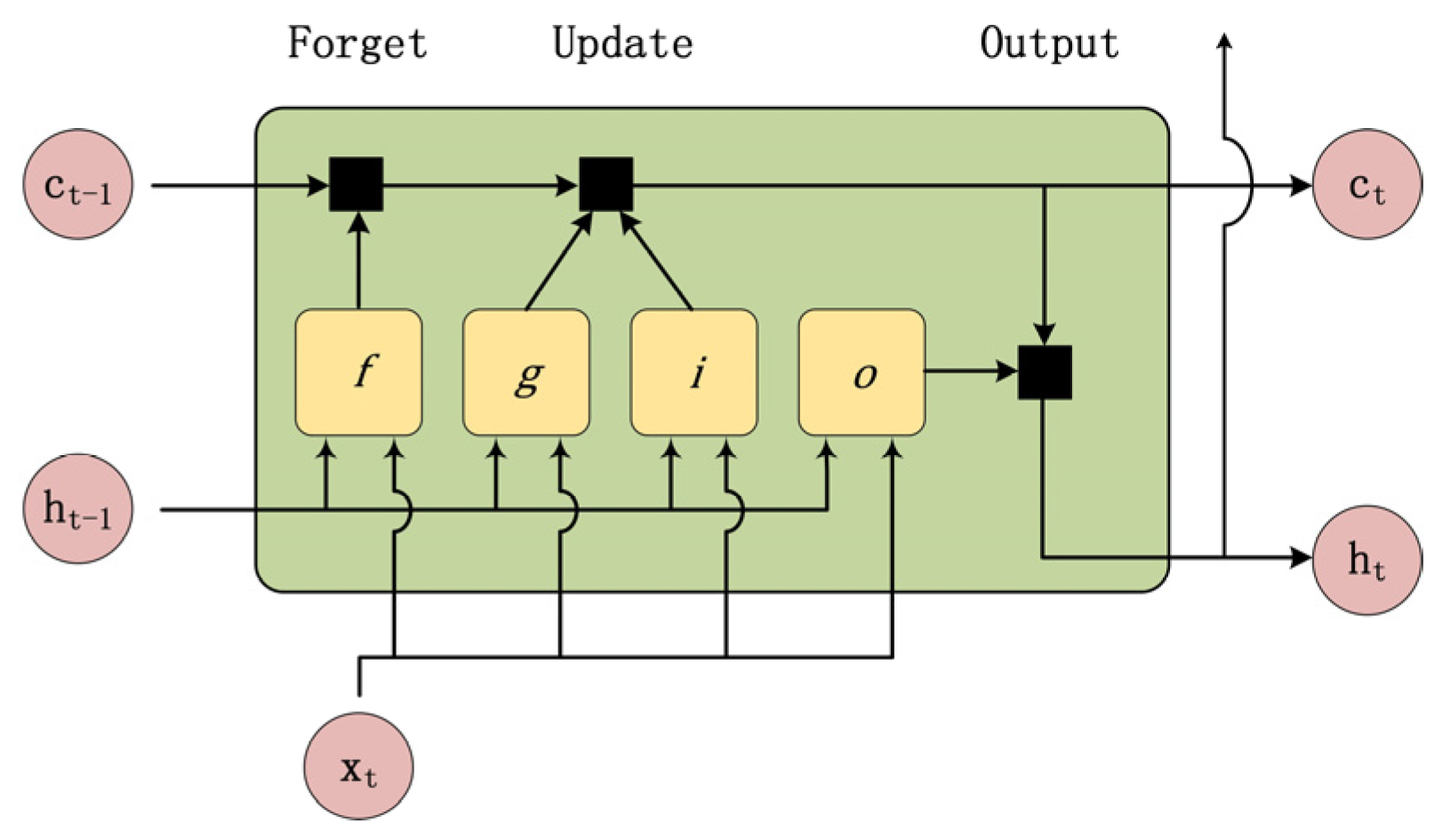
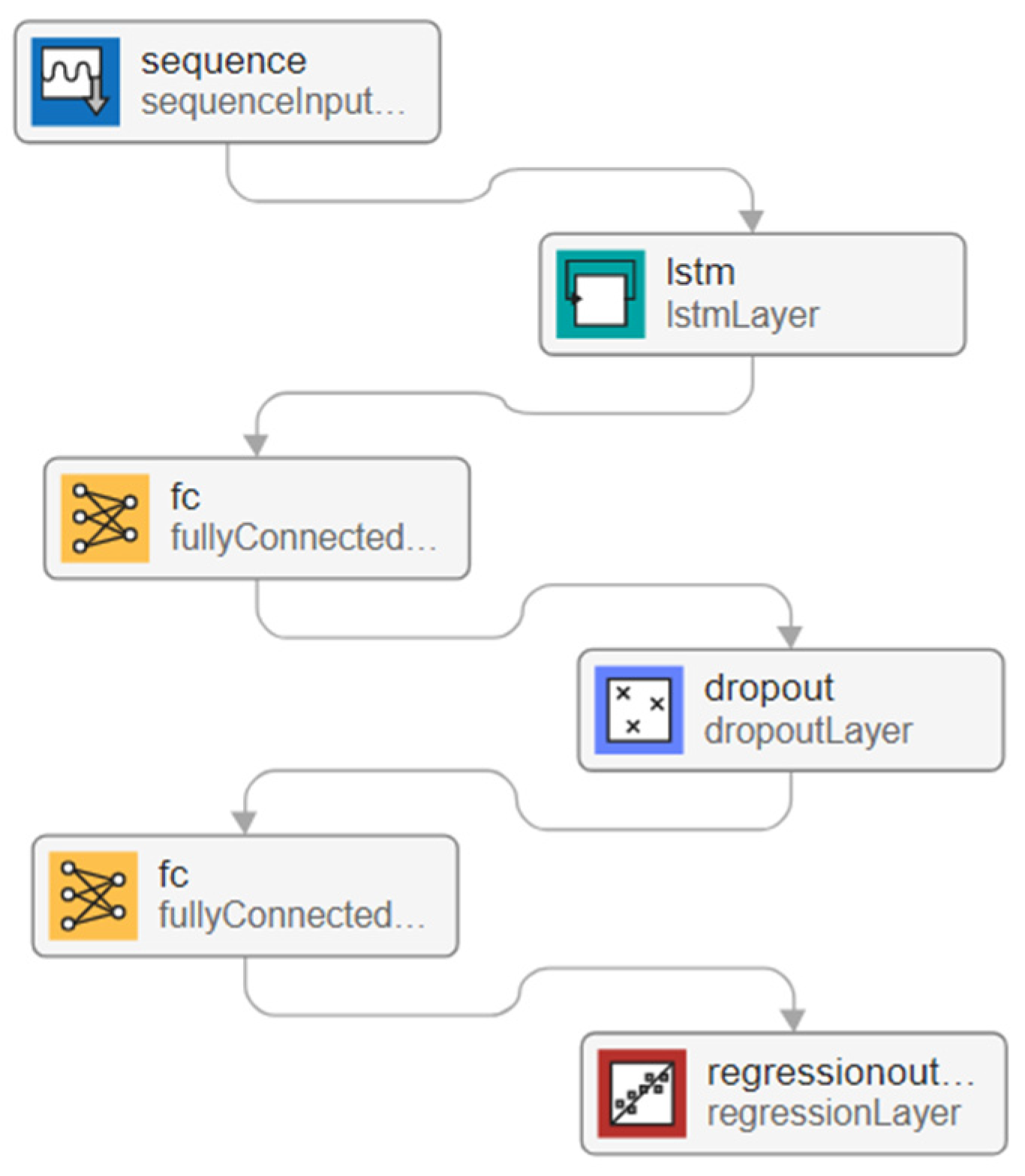
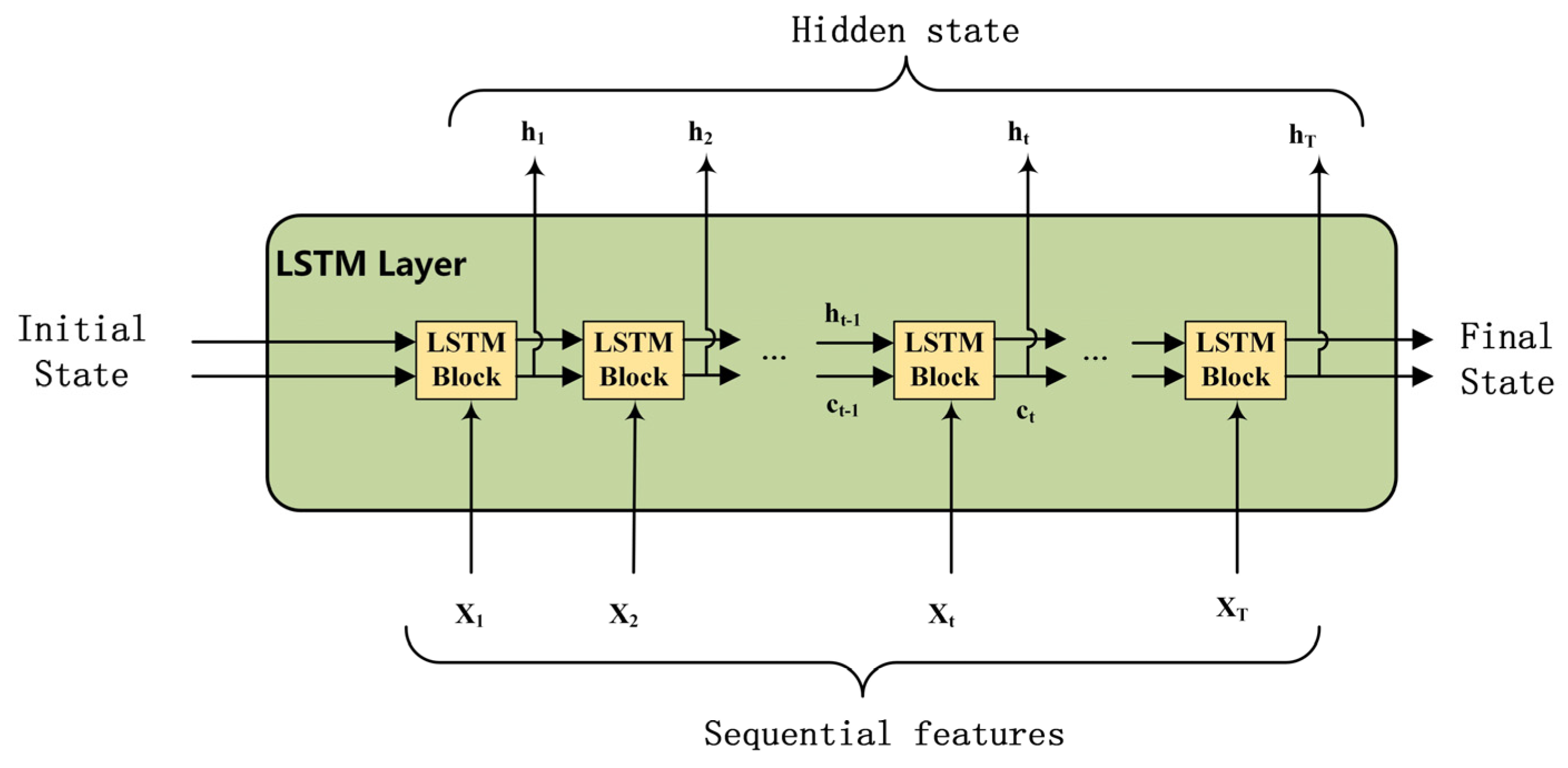
3. Tool Wear Monitoring with LSTM and the Multichannel Cutting Force Coefficients

Tool wear is a progressive degradation process. Sequential estimation, which combines current and historical information, is a good way to monitor progressive tool wear. LSTM (Long Short-Term Memory) is a type of recurrent neural network (RNN) architecture that is well-suited for learning long-term dependencies in sequences [22], as Figure 2 shows. Therefore, the LSTM model is utilized to monitor the tool wear from the extracted six cutting force coefficients.

Unlike the traditional RNNs, LSTMs have a memory cell that can maintain information over long time periods and prevent the vanishing gradient problem, which makes them more suitable for tasks such as speech recognition, natural language processing, and time series analysis. The key component of the LSTM architecture is the memory cell, which has three gates: the input gate, the forget gate, and the output gate. The input gate controls the flow of new information into the memory cell, the forget gate decides what information to keep and what to discard, and the output gate determines how the memory cell’s information is used, as Figure 3 shows. These gates are controlled by sigmoid activation functions and trained using backpropagation through time (BPTT). According to study [22], the mathematical representation of the LSTM can be written using Equations (9) and (10).

$$c_t=f_t\odot c_{t-1}+i_t\odot g_t$$

(9)

$$h_t=o_t\odot {\sigma }_c\left(c_t\right)$$

(10)

where i, f, g, and o denote the input gate, forget gate, cell candidate, and output gate, respectively. Notation ⊙ denotes the Hadamard product, and ${\sigma }_c$ denotes the state activation function.

According to the data form and the task, the LSTM can be categorized into four classes: sequence-to-label classification, sequence-to-sequence classification, sequence-to-one regression, and sequence-to-sequence regression. In this study, the continuous flank wear width (VB) was adopted to measure the tool wear state. Thus, the monitoring of the flank wear width was a regression problem. As the VB should be estimated at each time step, the monitoring process was a typical sequence-to-sequence regression process. As Figure 4 shows, the proposed LSTM has eight layers: the sequence input layer with the sequence of the six cutting force coefficients as the input, three LSTM layers with 13 hidden states, the fully connected layer with 10 notes, the dropout layer with a dropout probability of 0.5, the fully connected layer, and the regression layer. It is worth noting that the stacked LSTM form was adopted in this study to better represent the nonlinear regression relationship between the features and the flank wear. To avoid overfitting, only three LSTMs were stacked in this study.

The LSTM for tool wear monitoring was constructed with the guide of the Deep Learning Toolbox in MATLAB [23]. Before training the LSTM, the input data were normalized to have zero mean and unit variance. The training options were as follows: (1) train for 60 epochs with mini-batches of size 1 using the solver ‘Adam’; (2) the learning rate was set to 0.01; (3) the gradient threshold was set to 1 to prevent the gradients from exploding; and (4) ‘Shuffle’ was set to ‘never’ to keep the sequences sorted by length.

4. Experimental Validations and Analysis

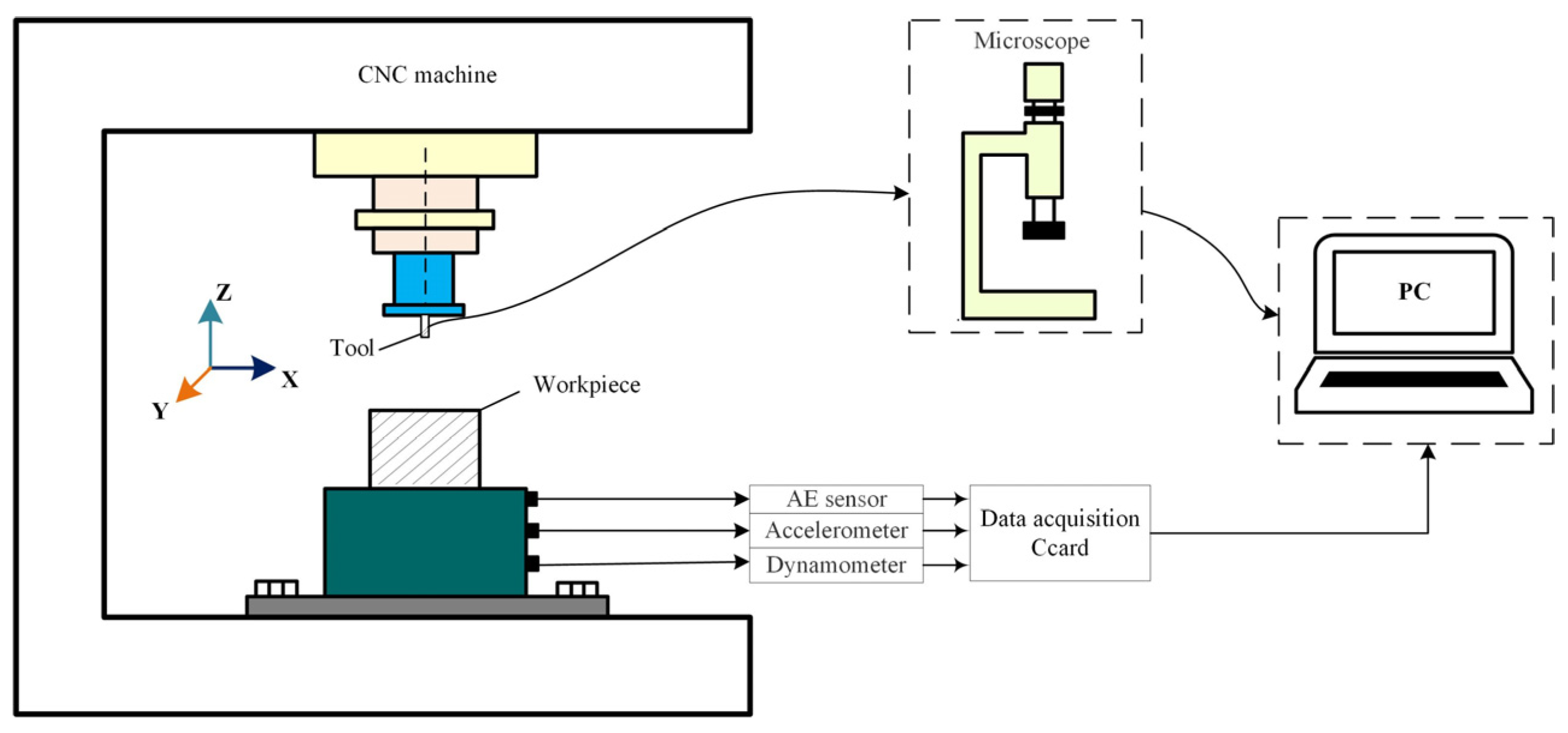
4.1. Experimental Setup

The data from PHM 2010 were adopted to validate the monitoring method. The PHM Data Challenge is a competition open to all potential conference attendees. The challenge in 2010 was focused on RUL estimation for high-speed CNC milling machine cutters using dynamometer, accelerometer, and acoustic emission data. The PHM 2010 tool wear data are often used to validate the monitoring method, as the data set has enough tool wear data. This study also adopted the data set to validate the multichannel coefficient-based tool wear monitoring method. In the milling experiment of PHM 2010, six ball nose milling tools were utilized. The six experiments were C1–C6. These cutters varied in terms of their geometry and coating, but they all shared the same specifications, including 6 mm alignment-tool carbide ball-nose ends with three flutes. The material in the cutting processes in this experiment was stainless steel (HRC52). During the cutting process, the upper face of the material was horizontally cut from top to bottom, which created a series of lines. After 315 cuts were completed, another cutter started again at the top edge and made another 315 similar cuts. The cutting face measured 112.5 mm wide and 40 mm high. The cutting parameters are listed in

Table 2. The cutting tool, material, and cutting parameters used in the experiments.

CNC Machine	Röders Tech RFM760 (Soltau, Germany)
Tool type	Ball nose milling cutter
Number of flutes	3
Workpiece material	Stainless steel (HRC52)
Spindle speed	10,400 rpm
Feed rate	1555 mm/min
Radial cutting depth	0.125 mm
Axial cutting depth	0.2 mm
Number of cuts per experiment	315

. The experiment setup is shown in Figure 5. Detailed information about the experimental setup can be found in reference [24].

The cutting force signal was collected using a dynamometer with three channels for the different directions, with a PCI1200 board with a sampling rate of 50 KHz per channel. The tool wear was measured after each cut and stored in the computer along with the sensed signals, which were captured using Labview software running on the computer. The Labview software could be found at https://www.ni.com/en/support/downloads/software-products/download.labview.html#521715 (accessed on 6 April 2024). Detailed information about the PHM 2010 data can be found at https://phmsociety.org/phm_competition/2010-phm-society-conference-data-challenge/ (accessed on 15 July 2023). Because the tool wear values in experiments C2, C3, and C5 were not measured, only the experimental data in C1, C4, and C6 were utilized. Three groups of training and testing were conducted. The training and testing data for the three groups are listed in

Table 3. The cutting parameters used in the experiments.

Number	Training Data	Testing Data
1	C4 and C6	C1
2	C1 and C6	C4
3	C1 and C4	C6

.

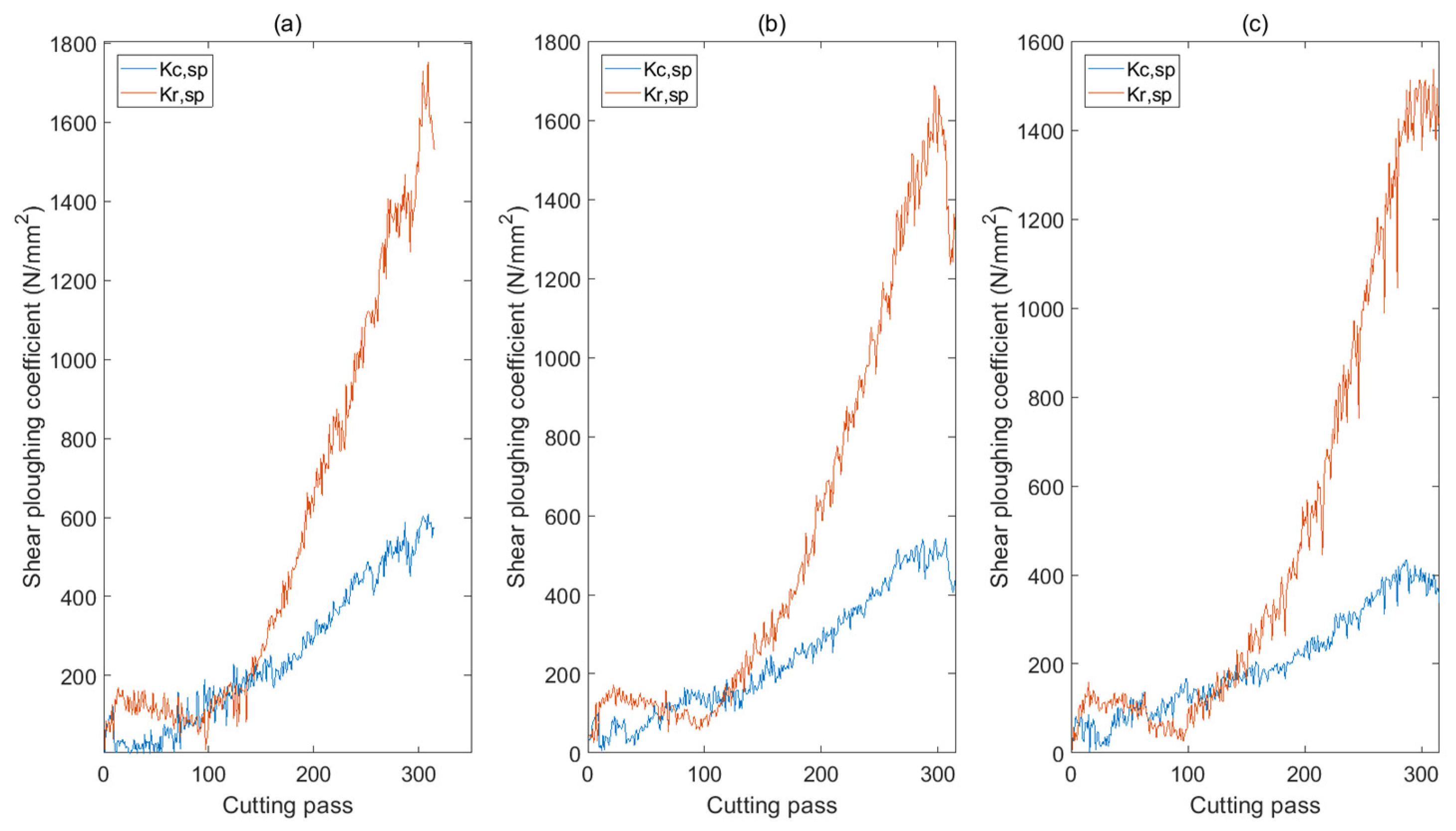
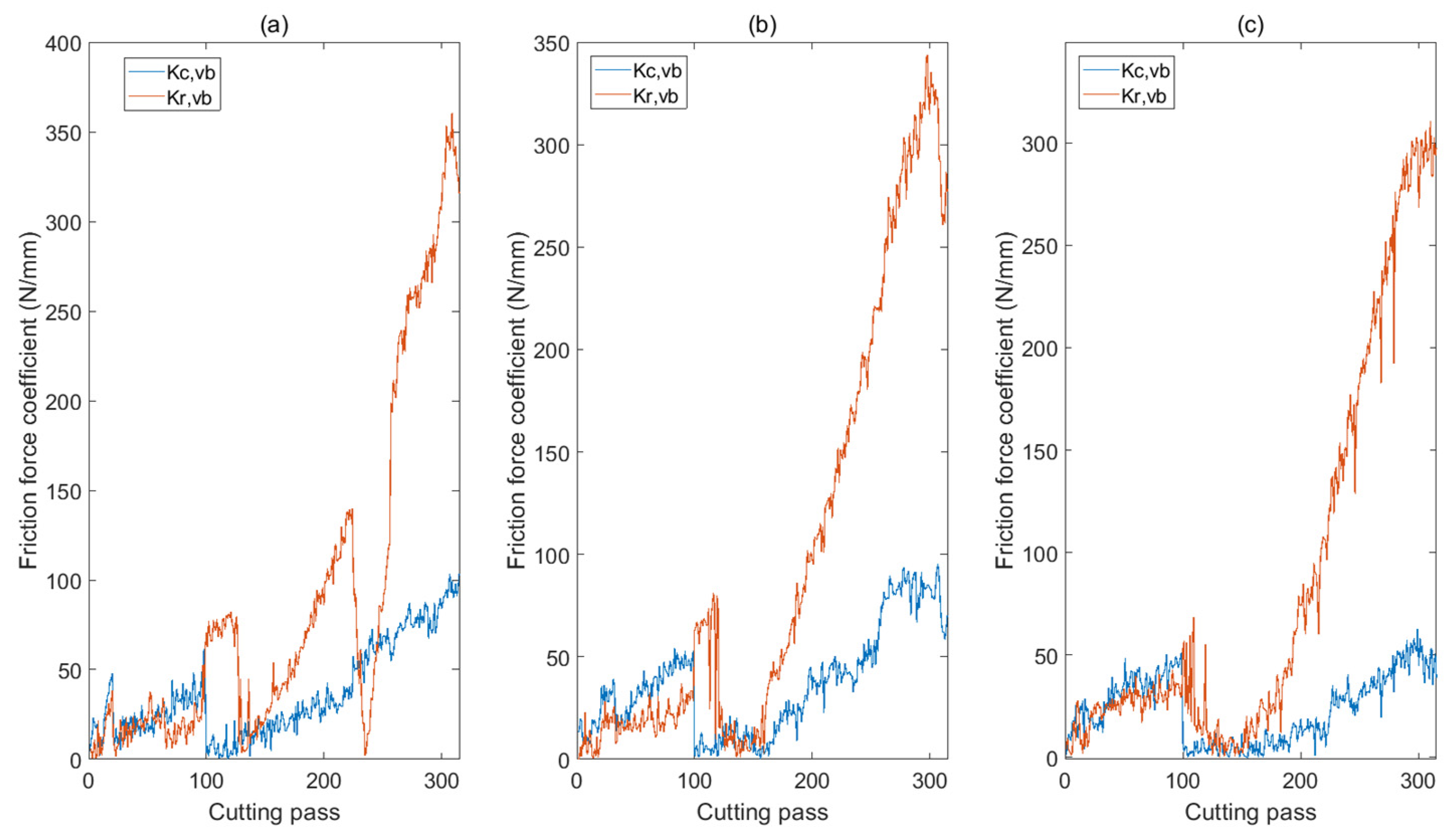
4.2. Tool Wear Feature Extraction and Analysis

The cutting forces with different tool wear conditions are shown in Figure 6, Figure 7 and Figure 8. The amplitude of force increased with the tool wear. The amplitude of the force Fx at the end pass (pass 315) was nearly 30 times the amplitude of the force with a fresh tool. This implies that tool wear indeed has a great impact on the cutting force. Among the forces in the three directions, the force Fz had the smallest amplitude. This is because the helix angle was small, and the effect of cutting on the axial direction was slight. Also, the waveform of the force at the first cutting pass was more irregular than the fore waveform with the worn tool. This may be because the tooltip was shaped at the first cutting pass, and the worn tool had a blunter tooth tip and a smoother waveform.

The extracted tangential and radial cutting force coefficients are shown in Figure 9 and Figure 10. Figure 9 shows the shear/ploughing coefficients, and Figure 10 shows the friction force coefficients. The figures clearly show that both the shear/ploughing coefficients and the friction force coefficients increase with the tool wear. This is because the uncut chip thickness does not vary with the tool wear, while the cutting force increases with the tool wear. From the two figures, it was also found that the shear/ploughing coefficient was bigger than the friction force coefficient. This is because the chip formation occurred in the shear/ploughing region and made the shear/ploughing force much bigger than the friction force in the flank wear region. Figure 11 presents the extracted axial cutting force coefficients. It shows that the axial coefficients are able to adequately indicate the tool wear condition. The standard deviation of the extracted cutting force coefficients is presented in Figure 12.

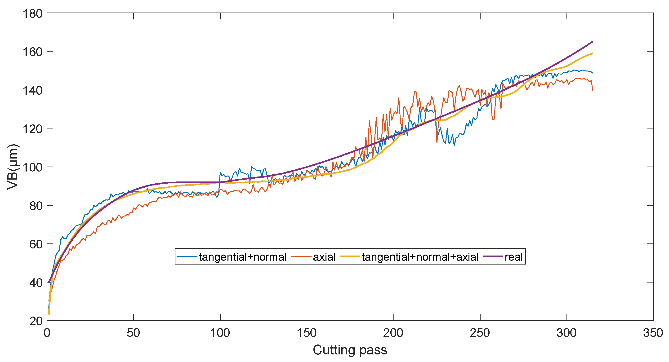
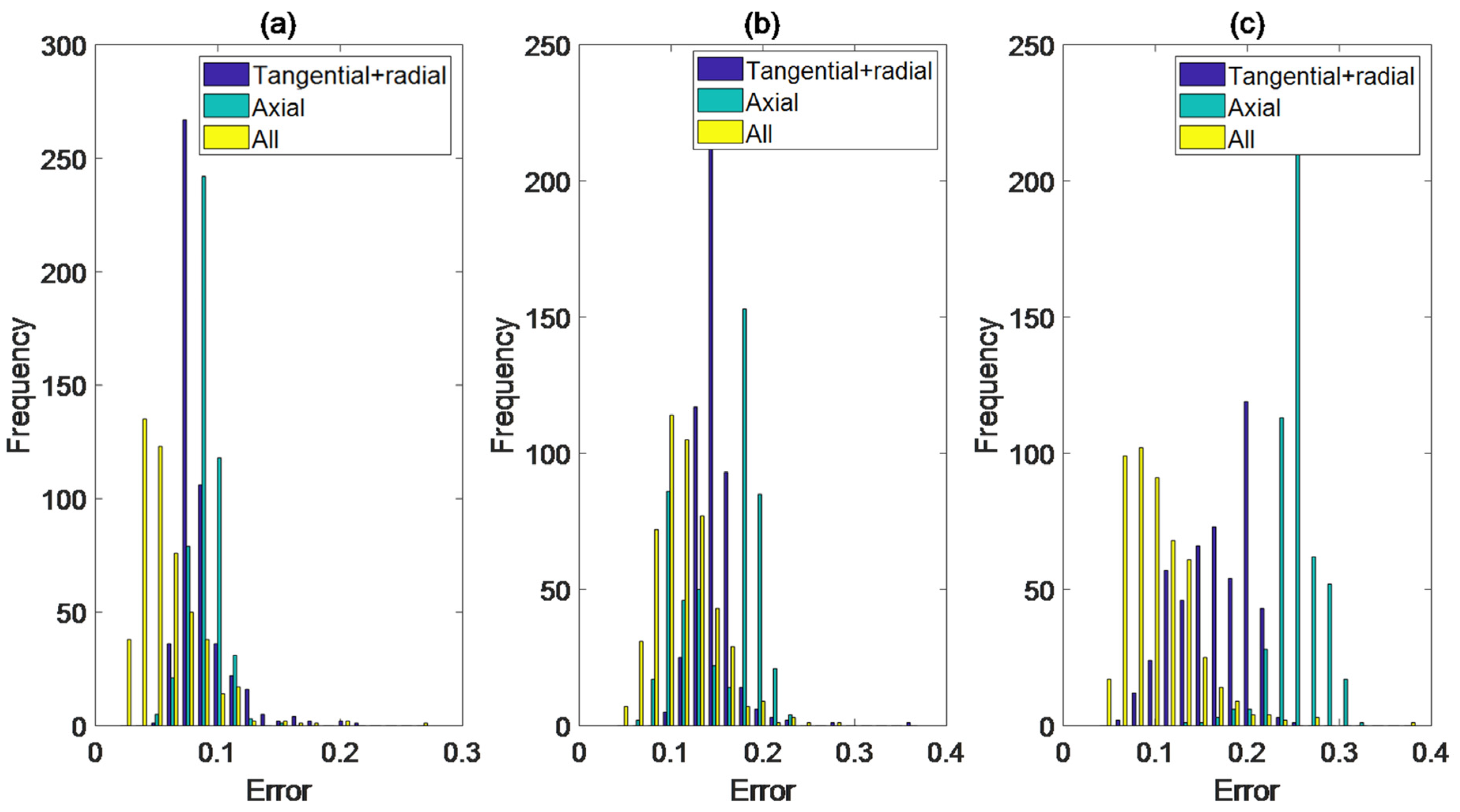
4.3. Tool Wear Monitoring Results and Analysis

The testing results are presented in Figure 13, Figure 14 and Figure 15. Figure 13 presents the testing results of C1, with C4 and C6 as the training sets. Figure 14 presents the testing results of C4, with C1 and C6 as the training sets. Figure 15 presents the testing results of C6, with C1 and C4 as the training sets. From the figures, it was found that the monitoring method via the fusion of the six cutting force coefficients had a higher tool wear estimation accuracy, especially for the monitoring of the severe tool wear condition at the last cutting passes. The relative monitoring error defined in Equation (11) was adopted to measure the monitoring accuracy.

$$Error=\frac{{\displaystyle \sum _{i=1}^P{\left(V{B}_{m,i}-V{B}_{r,i}\right)}^2}}{{\displaystyle \sum _{i=1}^{P}V{B}_{r,i}^2}}$$

(11)

where $V{B}_{m,i}$ is the monitored flank with a width at the i-th cutting pass, $V{B}_{r,i}$ is the real flank with a width at the i-th cutting pass, and P is the number of cutting passes.

The influence of the initial parameters on training process was analyzed by conducting multi-training with random initial parameters. Five hundred training processes were carried out for each experiment. The distributions of the monitored error are shown in Figure 16. The average error is listed in

Table 4. The average monitoring error with different coefficients.

Number	Tangential + Radial	Axial	Tangential + Radial + Axial
1	8.53%	8.98%	5.79%
2	14.70%	15.38%	11.33%
3	16.58%	25.39%	10.23%

. It shows that, compared to the traditional monitoring method with tangential and radial cutting force coefficients, the proposed monitoring method with the multichannel coefficients yielded more accurate monitoring results and improved the monitoring accuracy by 2.74–6.35%.

According to the results presented above, it can be concluded that although the axial force is small, the axial coefficients extracted from the axial force are sensitive to the tool wear condition, and incorporating the axial coefficients into the monitoring system improves the monitoring accuracy. The effectiveness of applying the stacked LSTM to the progressive tool wear monitoring was also verified by comparing the monitoring results of different models. The single-layer LSTM model and the commonly used MLP model were used for comparison purposes. The monitoring results via different models are presented in

Table 5. The average monitoring error of different monitoring models.

Number	MLP	Single-Layer LSTM	Stacked LSTM
1	10.37%	9.24%	5.79%
2	16.73%	14.95%	11.33%
3	16.58%	18.17%	10.23%

. It clearly shows that the stacked LSTM model yielded a more accurate monitoring result. This is because the stacked LSTM is better at representing the nonlinear relationship between the features and the tool wear and is also better at estimating the sequential tool wear progress compared to the single-layer LSTM and MLP models.

Although the multichannel coefficient-based method improves the monitoring accuracy, the average monitoring accuracy is still not satisfactory. This may be due to the existence of a non-neglected discrepancy between the training and testing experimental data, and the LSTM model that was trained using the two groups of experimental data cannot be directly used for the testing of the other data. In future work, we will study the discrepancy between the sequential tool wear data and build a transfer LSTM [25] to monitor the tool wear process to solve the discrepancy problem and to further improve the monitoring accuracy.

5. Conclusions

The multichannel cutting force coefficients, viz., the tangential, radial, and axial coefficients, extracted from the three-dimensional cutting force signals were fused to monitor the tool wear. A mechanistic cutting force model with the multichannel coefficients as the model parameters was constructed. The multichannel coefficients were extracted by identifying the mechanistic model. The LSTM model was adopted to estimate the tool wear value from the sequential coefficients. Some conclusions are as follows:

(1)

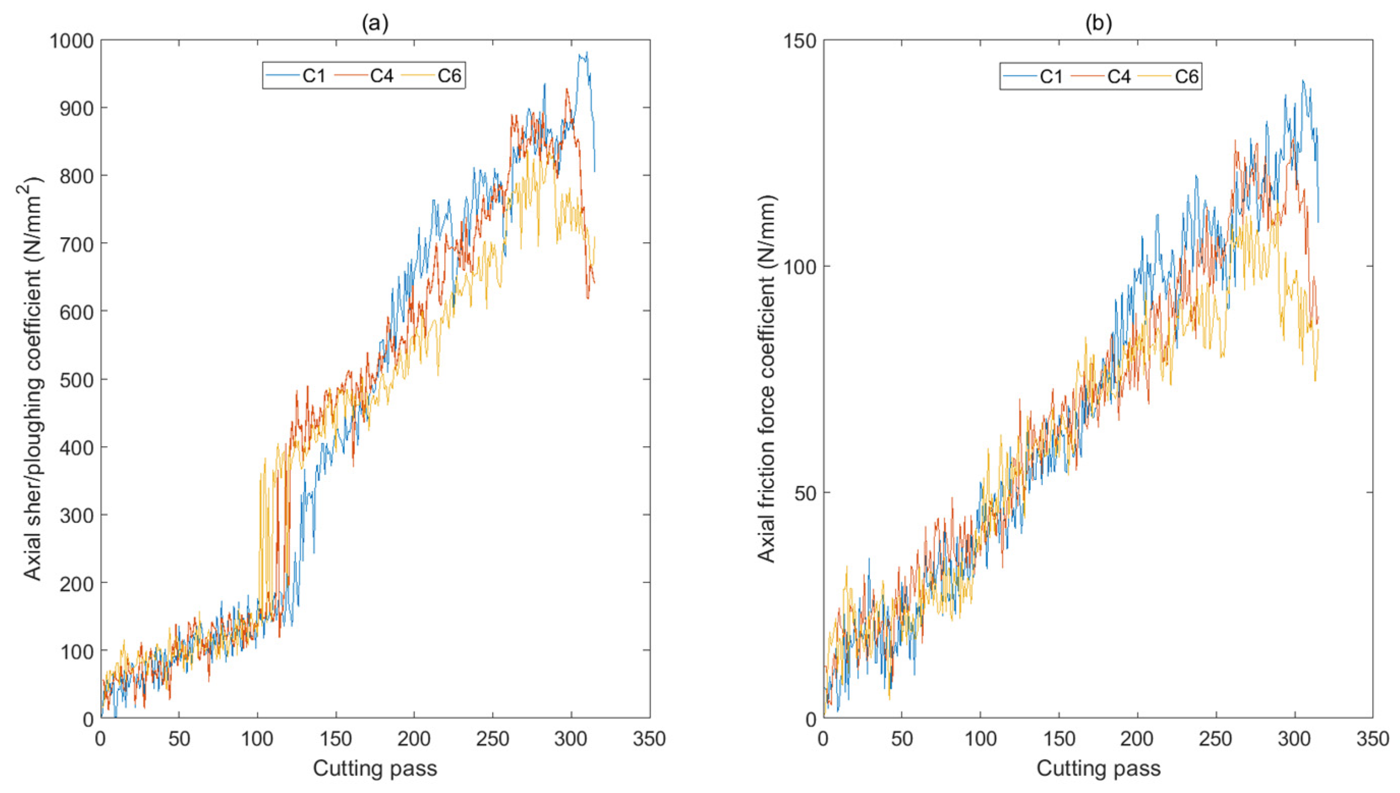
The tangential, radial, and axial cutting force coefficients were sensitive to the tool wear condition.

(2)

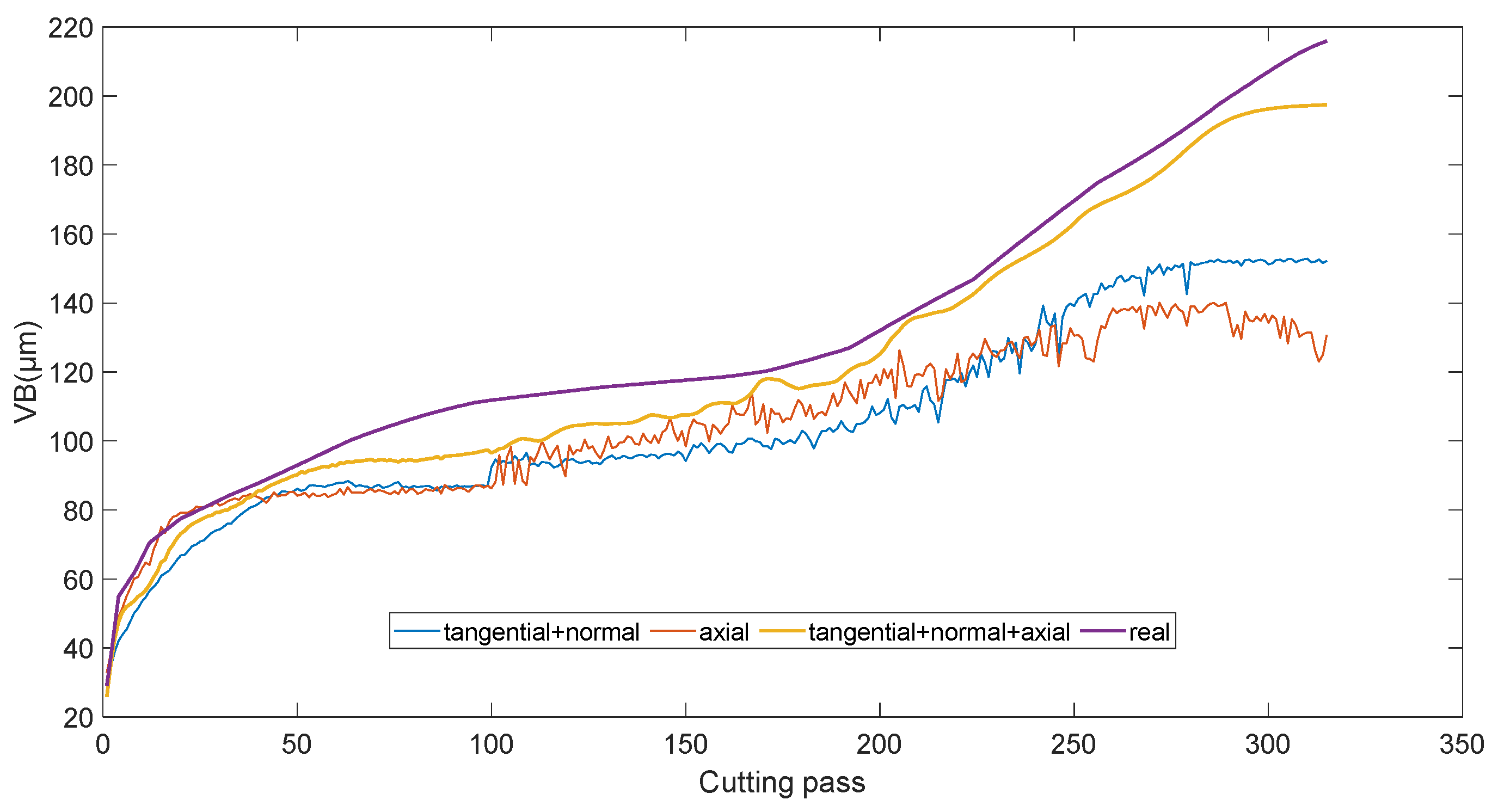
With the fusion of the multichannel cutting force coefficients, the monitoring accuracy improved by 2.74–6.35%.

(3)

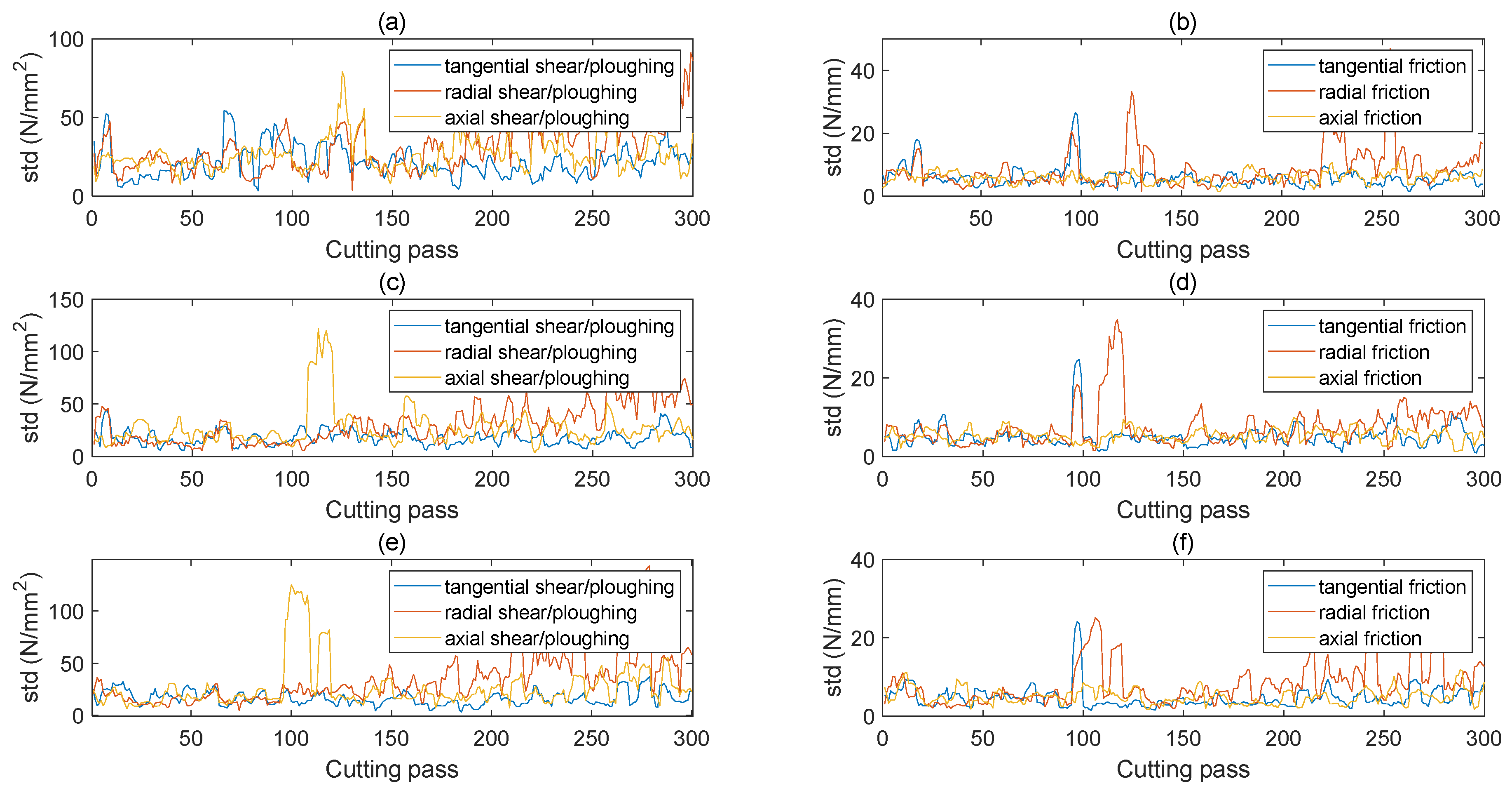
The shear/ploughing coefficient was bigger than the friction force coefficient and was more sensitive to the tool wear condition in milling Inconel 718.

The extraction of the multichannel cutting force coefficients relies on the analytical and regular cutting force model, and thus, the cutting force coefficient can be regarded as a regular feature of the cutting force signal. The irregularity and singularity of the cutting force signal, such as the fractal dimension and Holder exponent, can also indicate the tool wear condition and will be incorporated into the monitored model in future work. In addition, the transfer stacked LSTM model will be considered to solve the discrepancy problem and to further improve the monitoring accuracy.

References

1. Xie, Y.; Lian, K.; Liu, Q.; Zhang, C.; Liu, H. Digital twin for cutting tool: Modeling, application and service strategy. J. Manuf. Syst. 2021, 58, 305–312. [Google Scholar] [CrossRef]
2. Peng, Y.; Song, Q.; Wang, R.; Yang, X.; Liu, Z.; Liu, Z. A tool wear condition monitoring method for non-specific sensing signals. Int. J. Mech. Sci. 2024, 263, 108769. [Google Scholar] [CrossRef]
3. Liu, C.; Zhu, H.; Tang, D.; Nie, Q.; Zhou, T.; Wang, L.; Song, Y. Probing an intelligent predictive maintenance approach with deep learning and augmented reality for machine tools in IoT-enabled manufacturing, Robot. Comput. Integr. Manuf. 2022, 77, 102357. [Google Scholar] [CrossRef]
4. Zhu, L.; Liu, C. Recent progress of chatter prediction, detection and suppression in milling, Mech. Syst. Sig. Process. 2020, 143, 106840. [Google Scholar] [CrossRef]
5. Zhu, K.; Mei, T.; Ye, D. Online condition monitoring in micromilling: A force waveform shape analysis approach. IEEE Trans. Ind. Informat. 2015, 62, 3806–3813. [Google Scholar] [CrossRef]
6. Asadzadeh, M.Z.; Eib¨ock, A.; G¨anser, H.-P.; Klünsner, T.; Mücke, M.; Hanna, L.; Teppernegg, T.; Treichler, M.; Peissl, P.; Czettl, C. Tool damage state condition monitoring in milling processes based on the mechanistic model goodness-of-fit metrics. J. Manuf. Process. 2022, 80, 612–623. [Google Scholar] [CrossRef]
7. Hsieh, W.H.; Lu, M.C.; Chiou, S.J. Application of backpropagation neural network for spindle vibration-based tool wear monitoring in micro-milling. Int. J. Adv. Manuf. Technol. 2012, 61, 53–61. [Google Scholar] [CrossRef]
8. Liu, B.; Liu, C.; Zhou, Y.; Wang, D.; Dun, Y. An unsupervised chatter detection method based on AE and merging GMM and K-means. Mech. Syst. Sig. Process. 2023, 186, 109861. [Google Scholar] [CrossRef]
9. Díaz-Saldaña, G.; Osornio-Ríos, R.A.; Zamudio-Ramírez, I.; Cruz-Albarrán, I.A.; Trejo-Hernández, M.; Antonino-Daviu, J.A. Methodology for Tool Wear Detection in CNC Machines Based on Fusion Flux Current of Motor and Image Workpieces. Machines 2023, 11, 480. [Google Scholar] [CrossRef]
10. Zhang, X.; Gao, Y.; Guo, Z.; Zhang, W.; Yin, J.; Zhao, W. Physical model-based tool wear and breakage monitoring in milling process. Mech. Syst. Sig. Process. 2023, 184, 109641. [Google Scholar] [CrossRef]
11. Bernini, L.; Albertelli, P.; Monno, M. Mill condition monitoring based on instantaneous identification of specific force coefficients under variable cutting conditions. Mech. Syst. Sig. Process. 2023, 185, 109820. [Google Scholar] [CrossRef]
12. Sousa, V.F.C.; Silva, F.J.G.; Fecheira, J.S.; Lopes, H.M.; Martinho, R.P.; Casais, R.B.; Ferreira, L.P. Cutting forces assessment in CNC machining processes: A critical review. Sensors 2020, 20, 4536. [Google Scholar] [CrossRef] [PubMed]
13. Altintas, Y. Manufacturing Automation: Metal Cutting Mechanics, Machine Tool Variations, and CNC Design, 2nd ed.; Cambridge University Press: New York, NY, USA, 2012. [Google Scholar]
14. Lu, X.; Wang, F.; Jia, Z.; Si, L.; Zhang, C.; Liang, S.Y. A modified analytical cutting force prediction model under the tool flank wear effect in micro-milling nickel-based superalloy. Int. J. Adv. Manuf. Technol. 2017, 91, 3709–3716. [Google Scholar] [CrossRef]
15. Zhou, L.; Deng, B.; Peng, F.; Yang, M.; Yan, R. Semi-analytic modelling of cutting forces in micro ball-end milling of NAK80 steel with wear-varying cutting edge and associated nonlinear process characteristics. Int. J. Mech. Sci. 2020, 169, 105343. [Google Scholar] [CrossRef]
16. Nouri, M.; Fussell, B.K.; Ziniti, B.L.; Linder, E. Real-time tool wear monitoring in milling using a cutting condition independent method. Int. J. Mach. Tools. Manuf. 2015, 89, 1–13. [Google Scholar] [CrossRef]
17. Hou, Y.; Zhang, D.; Wu, B.; Luo, M. Milling force modeling of worn tool and tool flank wear recognition in end milling. IEEE/ASME Trans. Mechatron. 2014, 20, 1024–1035. [Google Scholar] [CrossRef]
18. Pan, T.; Zhang, J.; Zhang, X.; Zhao, W.; Zhang, H.; Lu, B. Milling force coefficients-based tool wear monitoring for variable parameter milling. Int. J. Adv. Manuf. Technol. 2022, 120, 4565–4580. [Google Scholar] [CrossRef]
19. Liu, T.; Zhu, K.; Wang, G. Micro-milling tool wear monitoring under variable cutting parameters and runout using fast cutting force coefficient identification method. Int. J. Adv. Manuf. Technol. 2020, 111, 3175–3188. [Google Scholar] [CrossRef]
20. Jing, X.; Lv, R.; Chen, Y.; Tian, Y.; Li, H. Modelling and experimental analysis of the effects of run out, minimum chip thickness and elastic recovery on the cutting force in micro-end-milling. Int. J. Mech. Sci. 2020, 176, 105540. [Google Scholar] [CrossRef]
21. Li, K.; Zhu, K.; Mei, T. A generic instantaneous undeformed chip thickness model for the cutting force modeling in micromilling. Int. J. Mach. Tool. Manu. 2016, 105, 23–31. [Google Scholar] [CrossRef]
22. Yu, Y.; Si, X.; Hu, C.; Zhang, J. A review of recurrent neural networks: LSTM cells and network architectures. Neural Comput. 2019, 31, 1235–1270. [Google Scholar] [CrossRef]
23. Beale, M.H.; Hagan, M.T.; Demuth, H.B. Deep Learning Toolbox; User’s Guide; The MathWorks, Inc.: Natick, MA, USA, 2018; Available online: https://research.iaun.ac.ir/pd/mahdavinasab/pdfs/UploadFile_4309.pdf (accessed on 1 May 2023).
24. Li, X.; Lim, B.S.; Zhou, J.H.; Huang, S.; Phua, S.J.; Shaw, K.C.; Er, M.J. Fuzzy neural network modelling for tool wear estimation in dry milling operation. In Proceedings of the Annual Conference of the PHM Society, San Diego, CA, USA, 27 September–1 October 2009; Volume 1. [Google Scholar]
25. Sagheer, A.; Hamdoun, H.; Youness, H. Deep LSTM-Based Transfer Learning Approach for Coherent Forecasts in Hierarchical Time Series. Sensors 2021, 21, 4379. [Google Scholar] [CrossRef] [PubMed]
Figure 1. The cutting force decomposition in milling process.
Machines 12 00249 g001
Figure 2. The data flowchart in the LSTM model.
Machines 12 00249 g002
Figure 3. The structure of the LSTM block.
Machines 12 00249 g003
Figure 4. The structure of the LSTM model for progressive tool wear monitoring.
Machines 12 00249 g004
Figure 5. Experiment setup.
Machines 12 00249 g005
Figure 6. The cutting force signal at the first cutting pass.
Machines 12 00249 g006
Figure 7. The cutting force signal at cutting pass 200.
Machines 12 00249 g007
Figure 8. The cutting force signal at cutting pass 315.
Machines 12 00249 g008
Figure 9. Shear/ploughing coefficients in tangential and radial directions: (a) C1; (b) C4; (c) C6.
Machines 12 00249 g009
Figure 10. Friction force coefficients in tangential and radial directions: (a) C1; (b) C4; (c) C6.
Machines 12 00249 g010
Figure 11. Cutting force coefficients in axial direction: (a) Shear/ploughing coefficients; (b) Friction force coefficients
Machines 12 00249 g011
Figure 12. The standard deviation of the extracted cutting force coefficients: (a) Shear/ploughing coefficients in C1; (b) Friction force coefficients in C1; (c) Shear/ploughing coefficients in C4; (d) Friction force coefficients in C4; (e) Shear/ploughing coefficients in C6; (f) Friction force coefficients in C6.
Machines 12 00249 g012
Figure 13. The monitoring results of C1.
Machines 12 00249 g013
Figure 14. The monitoring results of C4.
Machines 12 00249 g014
Figure 15. The monitoring results of C6.
Machines 12 00249 g015
Figure 16. The distribution of the monitoring error: (a) Experiment 1; (b) Experiment 2; and (c) Experiment 3.
Machines 12 00249 g016